Article

An Advisor-Based Architecture for a Sample-Efficient Training of Autonomous Navigation Agents with Reinforcement Learning

by
Rukshan Darshana Wijesinghe
1,2,*,
Dumindu Tissera
1,2,
Mihira Kasun Vithanage
2,3,
Alex Xavier
2,4,
Subha Fernando
2,3 and
Jayathu Samarawickrama
1,2
1
Department of Electronic and Telecommunication Engineering, Faculty of Engineering, University of Moratuwa, Moratuwa 10400, Sri Lanka
2
CODEGEN QBITS LAB, University of Moratuwa, Moratuwa 10400, Sri Lanka
3
Department of Computational Mathematics, Faculty of Information Technology, University of Moratuwa, Moratuwa 10400, Sri Lanka
4
Department of Computer Science and Engineering, Faculty of Engineering, University of Moratuwa, Moratuwa 10400, Sri Lanka
*
Author to whom correspondence should be addressed.
Robotics 2023, 12(5), 133; https://doi.org/10.3390/robotics12050133
Submission received: 23 August 2023 / Revised: 18 September 2023 / Accepted: 22 September 2023 / Published: 28 September 2023

Abstract

:
Recent advancements in artificial intelligence have enabled reinforcement learning (RL) agents to exceed human-level performance in various gaming tasks. However, despite the state-of-the-art performance demonstrated by model-free RL algorithms, they suffer from high sample complexity. Hence, it is uncommon to find their applications in robotics, autonomous navigation, and self-driving, as gathering many samples is impractical in real-world hardware systems. Therefore, developing sample-efficient learning algorithms for RL agents is crucial in deploying them in real-world tasks without sacrificing performance. This paper presents an advisor-based learning algorithm, incorporating prior knowledge into the training by modifying the deep deterministic policy gradient algorithm to reduce the sample complexity. Also, we propose an effective method of employing an advisor in data collection to train autonomous navigation agents to maneuver physical platforms, minimizing the risk of collision. We analyze the performance of our methods with the support of simulation and physical experimental setups. Experiments reveal that incorporating an advisor into the training phase significantly reduces the sample complexity without compromising the agent’s performance compared to various benchmark approaches. Also, they show that the advisor’s constant involvement in the data collection process diminishes the agent’s performance, while the limited involvement makes training more effective.

1. Introduction

Reinforcement learning (RL) is a trial-and-error-based learning method that learns to execute the best action while interacting with the environment. The agent takes action in each step, and the environment returns a scalar reward as feedback for the executed action. RL provides a framework to solve complex problems that are challenging to address with conventional methods. Recent advancements in RL have extended its applicability in various fields, such as gaming [1,2,3], recommendation systems [4], robotics [5,6,7,8], computer systems [9,10], and autonomous navigation [11,12,13]. Additionally, a number of advanced RL algorithms have outperformed human-level performance in diverse gaming environments [3,14], revealing the effectiveness of RL-based learning algorithms in addressing complex problems.
The penetration of RL into real-world applications began with the emergence of model-free algorithms such as deep-Q-network (DQN) [3], deep deterministic policy gradient (DDPG) [15], and twin-delayed DDPG (TD3) [16]. The DQN learns to control systems with discrete actions and continuous state variables, and the DDPG algorithm enables the agent to handle both states and actions in the continuous domain. TD3 is a variant of DDPG, derived from double-Q learning [17], and it utilizes two Q-value functions to minimize the overestimation bias and the accumulation of errors associated with Q-learning [16]. Despite the success showcased by model-free RL methods, end-to-end training demands significant sample complexity to achieve reasonable performance, as the agent is required to learn everything from scratch. Furthermore, the agent suffers from poor training performance with a high risk of failure at the initial stage due to the randomness of the actions predicted by the policy. As a result, their applications are mainly limited to simulation or virtual environment-based tasks, and it is rare to find RL-based applications in the fields that utilize physical platforms such as robotics, autonomous navigation, and self-driving [18].
Generally, the trial-and-error-based nature of RL makes it infeasible to use them for training autonomous navigation tasks in real-world settings. It is impractical to run many trials to collect a bulk of data and train an agent due to various practical issues such as regular maintenance caused by the wear and tear of mechanical parts, the requirement of the frequent charging and discharging of power sources, the difficulty in setting up the experimental setup for each trial, [19] etc. Also, the random behavior at the initial training phase introduces additional risk. Therefore, it requires safe and efficient (in terms of time, energy consumption, and cost) training procedures to employ RL-based agents with real-world platforms. Incorporating prior knowledge as an advisor in favor of safe and efficient training will be a promising strategy to minimize these issues. For example, consider the “goal reaching with obstacle avoidance” task in autonomous navigation. Despite our previous knowledge of the task and platform, the RL agents are generally required to learn basic navigation behaviors such as turning, driving straight, accelerating, and braking from scratch while interacting with the environment. However, these basic navigation behaviors are common for many tasks, and we know how to control the platform to achieve these behaviors. Learning them adds an extra exploration cost to the training and makes it inefficient. Also, the poor performance of the policy at the initial phase of the training does not guarantee safe training with minimal collisions. Therefore, incorporating the prior knowledge enhances the training performance of RL-based autonomous navigation agents.
The idea of transferring prior knowledge as an advisor during the training in the continuous domain has been introduced in [20]. It adapts the DDPG algorithm to incorporate an advisor to expedite the training process of continuous tasks. This paper compares the performance of transferring prior knowledge to train RL-based autonomous navigation agents with other state-of-the-art methods. In summary, the main contributions of this research are as follows.
  • Investigate the use of prior knowledge as an advisor to reduce the sample complexity of the DDPG and TD3 algorithms for autonomous navigation tasks in the continuous domain.
  • Devise an appropriate procedure to integrate the advisor role that makes the training of an autonomous navigation agent safer and more efficient.
  • Implement the proposed method with a physical experimental setup and analyze the performance on real navigation tasks.

2. Preliminaries

In the RL paradigm, an agent in state s t S at a given time step t interacts with an environment E as follows. The agent first executes an action a t A as predicted by a policy π : S P ( A ) , which maps states to a probability distribution over the actions. The agent receives an immediate scalar reward r t = r ( s t , a t , s t + 1 ) and then transitions to the next state s t + 1 according to a dynamic function f : S × A S . p ( s t + 1 , r t | s t , a t ) expresses the probability of transition to state s t + 1 after executing action a t in state s t . The goal of RL is to find a suitable policy π to maximize the expectation of the discounted future rewards R t = k = t γ k t r k received at a particular time step. γ is known as the discounting factor and 0 < γ < 1 . Thus, the state value function and the action value function are,
V π ( s ) = E [ R t | s t = s ; π ] Q π ( s , a ) = E [ R t | s t = s , a t = a ; π ]
The state value function is the expected total discounted reward of a state s, and the action value function represents the same for an action predicted a by a particular policy π in a given state s. The optimal policy that gives a maximum expected discounted reward can be expressed using the optimal action-value function as
π * ( s ) = a r g m a x a Q * ( s , a ) .
Similar to the above notation, V * ( s ) denotes the optimal state value function. The state value function can be written in a recursive form according to the “Bellman equations” [21] as follows:
v π ( s t ) = a t π ( a t | s t ) s t , r t p ( s t + 1 , r t | s t , a t ) [ r t + γ v π ( s t + 1 ) ]
Similarly, the action-value function can also be written in the recursive form of,
Q π ( s t , a t ) = s t , r t p ( s t + 1 , r t | s t , a t ) [ r t + γ a t + 1 π ( a t + 1 | s t + 1 ) q π ( s t + 1 , a t + 1 ) ]

3. Related Work

Introducing temporal difference methods in optimal control problems with trial and error-based learning approaches has laid the foundation for modern RL [21]. However, the applicability of RL was limited to the low dimensional discrete action and state spaces until the emergence of the deep Q-network [3]. Later, the DDPG algorithm was developed to handle a continuous high dimensional state and action spaces by combining DQN and a deterministic policy gradient [15,22]. These ground-breaking RL algorithms are capable of surpassing human-level performance in a variety of gaming environments. Integrating DDPG with the actor–critic [23] model allows for the learning of parameterized continuous policies, which are derived in terms of a parameterized Q-value function [15]. Double Q-learning addresses the effect of function approximation errors in actor–critic settings [24]. T. Haarnoja et al. [25] overcome the sample inefficiency and convergence in conjunction with maximum entropy RL used in off-policy actor–critic methods. A continuous variant of the Q-learning algorithm was combined with learned models to address the sample complexity in continuous domains [26]. Mehdi et al. [27] present a top-down approach for constructing state abstractions for reinforcement learning that makes learning more sample-efficient in the discrete domain. However, none of the above efforts are efficient enough to perform tasks associated with real platforms due to high sample complexity.
Despite the success exhibited, the applicability of the model-free RL algorithms has been limited in the autonomous navigation domain due to the difficulties caused by high sample complexity. Wen et al. [28] combine model-based RL algorithms with SLAM (simultaneous localization and mapping) to enhance the training efficiency of path planning and obstacle avoidance tasks. Tai et al. [29] propose a deep RL-based end-to-end asynchronous training approach for mapless navigation. Kahn et al. [30] propose a self-supervising generalized computational graph to enhance the sampling efficiency by subsuming the advantages of both model-free and model-based methods. Furthermore, Nagabandi et al. [31] combine a model-predictive controller and model-free learner to reduce the number of samples for the training. However, these methods require additional training with random policies to identify the model. Also, the uncertainties associated with learned models do not guarantee a safe training process.
Interactive reinforcement learning (IntRL) is an intriguing domain integrating a trainer to guide or evaluate the behavior of a learning agent [32,33]. The trainer’s advice reinforces the agent’s learning method and molds the exploration strategy, resulting in sample-efficient training by reducing the search spaces of states and actions [34]. Millan-Arias et al. [35] developed an actor–critic RL agent that trained in a disturbed environment while receiving advice, allowing the agent to learn more robust policies. Additionally, Bignold et al. [36] introduced a persistent rule-based approach for IntRL. This method aims to retain and reuse provided knowledge to reduce the interaction between the learner and the trainer by allowing trainers to give general advice for similar states. However, a rule-based advisor may cover only a limited search space of states and actions on complex navigation tasks.
Transferring knowledge from experts is one of the most effective methods to enhance training efficiency. Successor-feature-based RL is used in [37] to transfer knowledge across similar navigational environments to gain higher adaptability and lower training time. Emilio et al. [38] introduced a multitasking and transfer learning approach that allows an autonomous agent to simultaneously learn multiple tasks and then generalize the learned knowledge to new domains. Finding a suitable trained model to apply transfer learning is a challenging task. Therefore, Ross et al. [39] have incorporated the DAGGER algorithm, which uses a dataset of trajectories collected using an expert to initialize policies. Amini et al. [40] present a data-driven simulation and training engine capable of learning end-to-end autonomous vehicle control policies leveraged by human-collected trajectories. Kabzan et al. [41] employ a relatively simple vehicle model, which is improved based on measurement data and tools from machine learning, to perform autonomous racing. Taylor et al. [42] propose a method to increase the training speed of RL by mapping the knowledge gained in different tasks. However, leveraging the training of complex tasks with the knowledge gained in similar tasks may not support the navigation of physical platforms as it requires additional training. Also, employing a human as an expert may not always be advantageous for complex navigation tasks, especially when humans and robots perceive the environment differently.
Integrating imitation learning (IL) into RL has become a promising method of overcoming sample complexity by collecting data with the assistance of an expert [43,44,45]. Self-imitation learning in [46] reproduces the past good decisions of the agent to improve the exploration. Nair et al. [47] overcome exploration bottlenecks of the DDPG algorithm with Hindsight experience replay in simulated robotics tasks. Hester et al. use small demonstration data sets to accelerate deep Q learning [48]. Kahn et al. [49] present BADGR—Berkeley autonomous driving ground robot, an end-to-end self-supervised learning-based mobile robot navigation system that gathers data autonomously with minimal human supervision. However, the above approaches require learning everything from scratch and do not facilitate gaining the advantage of previous knowledge related to the task or navigation platform. In contrast, our approach incorporates prior knowledge of the task as an advisor for both exploration and exploitation to ensure the quick and safe training of autonomous navigation tasks.

4. Incorporating an Advisor

We propose an actor–critic model-based architecture that enables plugging an advisor (see Figure 1) to improve the training efficiency of model-free RL algorithms such as DDPG and TD3. In this approach, any set of rules, existing relationships, or pre-trained policies that map the states to actions can play the advisor role. The advisor used in this approach needs to have some knowledge related to the task, and it is not required to be capable of completing the task successfully. Our experiments use an advisor combining conventional goal-reaching methods with the classical Braitenberg navigation strategy [50] to maneuver a robotic platform to a given goal while avoiding obstacles. The implementation of the advisor and the navigation agent is explicitly described in Section 5.5.
The proposed architecture has two ways of employing an advisor in training. In the first method, the advisor guides the agent in data collection to explore the regions of the state and action spaces that return high rewards during the initial training phase while ensuring fewer failures. Secondly, the advisor assists the agent in policy updating to converge its policy toward a better policy that collects higher rewards by exploiting the advisor’s knowledge. However, in the event of the advisor’s suggestion being unavailable for a particular state, only the actor’s action must be considered for the data collection and policy updating processes. To investigate how the advisor influences the training efficiency of an RL-based autonomous navigation agent, we develop three types of agents that use the advisor: (1) only for the data collection, (2) only for the policy updating, and (3) for both the policy updating and data collection. We implement all these agent types by relying on the DDPG algorithm. Also, the developed policy updating and data collection methods are extended for TD3, a variant of DDPG, to achieve better performance.

4.1. Actor–Critic Model-Based Architecture

The architecture shown in Figure 1 is developed based on the actor–critic model [51], which comprises two main components called actor and critic. Policy π ( s ) plays the actor’s role and learns to produce the best action for a given state s at a particular time-step t. The critic aims to improve the actor’s behavior considering the rewards received from the environment for the action a played by the agent. The Q-value function Q ( s , a ) plays the critic’s role and gets updated using the temporal difference error [23]. In our implementation, we use neural networks to parameterize the policy and Q-value functions, and we refer to them as “actor-network” π ( s ; ϕ ) and “critic-network” Q ( s , a ; θ ) , respectively ( ϕ and θ represent the trainable parameters of the actor and critic networks, respectively). Additionally, we maintain another two neural networks to stabilize the learning process, similarly to the original DDPG algorithm [15]. They are known as “target actor-network” π T ( s ; ϕ T ) and “target critic-network” Q T ( s , a ; θ T ) , parameterized by ϕ T and θ T , respectively. These target networks are identical to the respective actor and critic networks in terms of architecture but different in terms of parameter updating methods. A soft updating method updates both target networks with the updating rate τ ( 0 < τ 1 ). The network architectures of the actor-network and critic-network used for the experiments are explained in detail in Section 5.3.
The updating procedure of the actor and critic networks is similar to the original DDPG algorithm [15] other than incorporating the advisor’s suggestions to update the actor-network. Also, we employ an asynchronous training method [29,52,53], expecting a quick convergence of both the actor and critic networks. Asynchronous training utilizes two parallel processes for the data collection and parameter updating of neural networks.

4.2. Data Collection Process

The method we use to employ the advisor for the data collection of navigation tasks is presented in Algorithm 1. As indicated by the architecture shown in Figure 1, the agent receives actions suggested by the actor ( a a c t ) and advisor ( a a d v ). The selector module of the architecture compares those two actions by considering the current knowledge (Q-value function) of the agent ( Q a d v and Q a c t represent the Q-value corresponding to the actor’s and advisor’s actions for the current state, respectively). The advisor’s action is selected for the execution if Q a d v is greater than Q a c t . Otherwise, the advisor’s or actor’s suggestion is selected for the execution with the probabilities of ϵ and ( 1 ϵ ) , respectively. We set a higher value for the advisor’s starting execution probability ϵ t s as the advisor demonstrates better performance than the actor at the initial stages of the training.
ϵ = 1 ( Q a c t Q a d v ) ( N N T ) ϵ s t b N ( Q a c t > Q a d v ) ( N N T ) 0 N > N T
We compute the advisor’s selection probability ϵ as given in Equation (1). N is the current episode number, and the starting probability ϵ s t is set to a higher value to guarantee a safe exploration with the advisor’s knowledge in the initial training stage. The selection probability of the advisor gradually reduces at the rate of b (b is a positive constant) when the episodes are progressing. Since ( 1 ϵ ) is the selection probability of the actor’s action, it gradually increases, and the actor’s action is selected for execution more frequently when the actor learns a better policy than the advisor. The agent entirely neglects the advisor’s action when episode number N exceeds the terminal episode of the advisor, N T . Then, Ornstein–Uhlenbeck [54] process-based noise is added to the selected action before the execution to ensure a better exploration. The agent executes the action calculated at the 14th step and observes the next state s and reward r returned from the environment. Finally, the tuple ( s , a , a a d v , s , r ) is stored as an experience in the memory replay buffer.
Algorithm 1 Data collection with an advisor
  1:
Initialize total number of training episodes N t o t a l
  2:
Initialize terminal episode number of the advisor N T
  3:
Initialize advisor’s starting execution probability ϵ s t
  4:
for  1 : N : N t o t a l   do
  5:
      Load the policy π ( s ; ϕ ) (actor-network) from the policy updating process
  6:
      Load the Q-value function Q ( s , a ; θ ) (critic-network) from the policy updating process
  7:
      while episode is not terminated do
  8:
            Observe current state s
  9:
            Calculate advisor’s action a a d v f ( s )
10:
            Calculate actor’s action a a c t π ( s ; ϕ )
11:
            Calculate advisor’s execution probability ϵ
12:
            With probability ϵ , a a a d v or otherwise, a a a c t
13:
             a a + n o i s e
14:
            Execute action a
15:
            Observe next state s and reward r
16:
            Store ( s , a , a a d v , s , r ) in the memory replay buffer

4.3. Policy Updating Process

Algorithm 2 describes how we incorporate the prior knowledge of the task into the policy updating process as an advisor by modifying the DDPG algorithm. It describes our method to update the actor-network (the policy), critic-network, and their respective target networks. We take the DDPG algorithm as the base for the modifications for explanation purposes. Also, Algorithm 2 can be easily extended to the advanced variants of DDPG, like TD3, that perform better than the original DDPG.
Algorithm 2 Policy updating with an advisor
  1:
Create actor-network π ( s ; ϕ ) and target actor-network π T ( s ; ϕ T )
  2:
Create critic-network Q ( s , a ; θ ) and target critic-network Q T ( s , a ; θ T )
  3:
Initialize actor and critic networks’ parameters ( ϕ and θ ) with He initialization
  4:
Initialize target networks’ parameters;
       ϕ T ϕ
       θ T θ
  5:
repeat:
  6:
       Sample a batch of experiences B = < S , A , A a d v , R , S > randomly from memory
       replay buffer with the size of n
  7:
       Set Q ^ R + γ Q T ( S , π T ( S ; ϕ T ) ; θ T )
  8:
       Update θ by minimizing the loss function L Q
              L Q = 1 n Σ [ Q ^ Q ( S , A ; θ ) ] 2
  9:
       A a c t π ( S ; ϕ )
10:
       A ^ A a c t + β A Q ( S , A a c t ; θ )
11:
       for  1 : i : n  do
12:
             if  Q ( s i , a a d v i ; θ ) > Q ( s i , a ^ i ; θ )  then
13:
                   a ^ i a a d v i
14:
       Update ϕ by minimizing the loss function L π
                L π = 1 n Σ [ A ^ π ( S ; ϕ ) ] 2
15:
       Update target networks parameters
                ϕ T τ ϕ + ( 1 τ ) ϕ T
                θ T τ θ + ( 1 τ ) θ T
16:
       Save all the networks
The policy updating process starts with fetching a randomly selected batch of stored tuples B = ( S , A , A a d v , R , S ) with the sample size of n from the memory replay buffer. Here, the uppercase symbols S , A , A a d v , R , and S represent batches of the variables s , a , a a d v , r , and s , respectively. We incorporate the gradient ascent technique in order to improve the current policy as given in Equation (2).
a ^ π ( s ; ϕ ) + β a Q ( s , a ; θ ) | s = s , a = π ( s )
Equation (2) calculates a target prediction a ^ for the policy function in terms of the Q-value gradient with respect to action a Q ( s , a ; θ ) . Here, the  β ( β > 0 ) represents the updating rate of the current policy. Step 10 of Algorithm 2 computes a set of improved target predictions A ^ for the selected batch using Equation (2). The individual target prediction a ^ A ^ is further improved in steps 12 and 13 by comparing it against the advisor’s actions a a d v considering the respective Q-values. For example, consider that the i t h samples of S , A ^ , and A a d v are s i , a ^ i , and a a d v i , respectively. If  Q ( s i , a ^ i ; θ ) < Q ( s i , a a d v i ; θ ) , then a ^ i is replaced with a a d v i , and this comparison is made for all the samples in A ^ . This basically improves the target predictions further with the help of the advisor’s knowledge related to the task. Throughout this paper, we refer to Algorithm 2 as the adapted DDPG (ADDPG) algorithm when the advisor’s actions are not considered during the policy updating process (without steps 12 and 13 of Algorithm 2).
Since the target predictions set A ^ contains samples of an improved policy function, we use them to update the current policy. Therefore, step 14 of Algorithm 2 updates the actor-network parameters ϕ by performing a single back-propagation step across the actor-network to minimize the loss function L π given in Equation (3). L π represents the averaged L-2 distance between the samples of current policy and target predictions modified with the advisor’s actions.
L π = 1 n [ A ^ π ( S ; ϕ ) ] 2
The updating method of the critic network is carried out based on the temporal difference error similar to the original DDPG algorithm [15]. We use two parameterized Q-value functions: critic-network Q ( s , a ; θ ) and target critic-network Q T ( s , a ; θ T ) . Similarly, there are two parameterized policy functions named actor-network ( π ( s ; ϕ ) ) and target actor-network π T ( s ; ϕ T ) . Equation (4) computes a set of target values Q ^ for the critic-network. Its parameters θ are updated by minimizing the loss function given in Equation (5). γ represents the discount factor and is set to 0.9 in all our experiments.
Q ^ = R + γ Q T ( S , π T ( S ; ϕ T ) ; θ T )
L Q = 1 n [ Q ^ Q ( S , π ( S ; ϕ ) ; θ ) ] 2
A soft updating method [15] is used to update the parameters of both target actor and critic networks as given in Equations (6) and (7). τ ( 0 < τ 1 ) controls their updating rates, and setting a smaller value (we set τ to 0.1 in our experiments) makes the learning more stable [15].
θ T = τ θ + ( 1 τ ) θ T
ϕ T = τ ϕ + ( 1 τ ) ϕ T

5. Experiment Setup

We conduct a series of experiments to evaluate the performance of the advisor-based architecture and check its applicability in the autonomous navigation domain. We use both simulation and real-world navigation platforms for the evaluation. We develop three advisor-based trainable agents that use the advisor for data collection, policy updating, and both data collection and policy updating. Each agent is trained to navigate a mobile robot platform to a predefined goal while avoiding obstacles. The starting and the goal positions are assigned randomly at the beginning of each episode. Agents are not provided with any other information related to the environment. All agents are required to learn to perform the given navigation task while interacting with the environment. We repeat every experiment six times to ensure the reliability of results and consider the average performance for the analysis. In simpler terms, each data point in any table or graph in the article is obtained by training six agents end-to-end. We used the simulation setup to understand how the advisor influences the agent’s training process, and we used the physical setup to verify the applicability of the proposed advisor-based architecture for real-world navigation tasks.

5.1. Simulation Setup
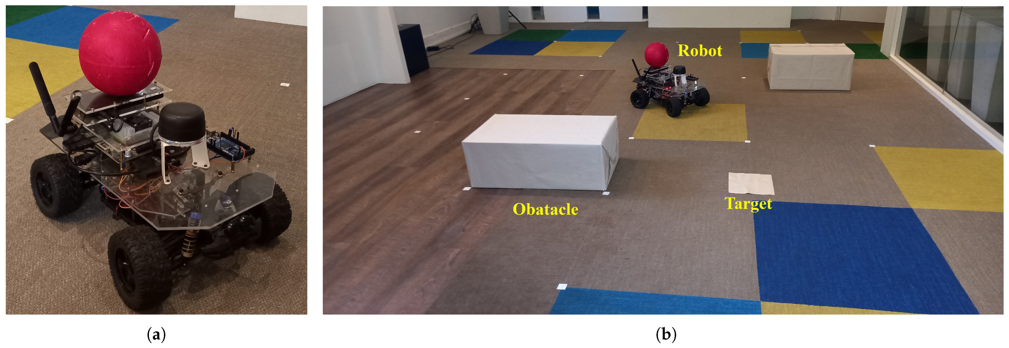
The simulation platform V-rep V3.6.2 (virtual robot experimentation platform) [55] is used to implement the simulation-based experimental setup. The Pioneer-3DX mobile robot is deployed as the navigation platform. The V-rep remote API for Python is used to communicate with the navigation agents. Each agent is trained to navigate the robot toward the target position (the red color square in Figure 2). The navigation platform has 16 proximity sensors around it to sense the presence of an obstacle or boundary wall near the robot. Two different simulation environments are used for training and validation purposes. Each environment differs from the other in terms of the number of obstacles and the gap between them (see Figure 2). Compared to the robot’s physical dimensions, having obstacles with sharp edges and lower gaps between obstacles and boundary walls makes the task more challenging. Also, having a small number of proximity sensors to observe the environment makes learning more difficult. A personal computer (PC) system with an Intel Core i5 CPU, and 8 Gb RAM is used to run the simulation-based experiments.

5.2. Physical Setup

We modify a Remo Hobby 1035 1 / 10 RC car into a navigation platform shown in Figure 3a to check the advisor-based architecture’s applicability on real navigation tasks. The platform is equipped with an RPLIDAR A2 laser scanner to measure the distance between obstacles and the platform. On average, the laser scanner gives 200 readings per rotation, and they are divided into 16 zones according to the angle corresponding to each reading. The minimum reading corresponding to a particular zone represents the obstacle distance associated with the zone, and we obtain such 16 distance measurements to perceive the environment. This whole process of reducing the resolution of distance readings makes the proximity measurements taken with the actual setup similar to the simulation. A NVIDIA Jetson TX2 developer board (NVIDIA Pascal architecture GPU module) was installed on the platform to make necessary computations associated with neural networks and execution of the trained policy. To estimate the platform’s position, we used an external personal computer (a system with Intel Core i5 CPU and 8 Gb RAM) to track the position of the red color ball fixed on the robot. We developed a blob analysis-based image processing method [56] to track the ball position by processing images from RGB cameras. Figure 3b shows the physical setup arranged to train agents. The robot and the tracking system communicate through WiFi to transfer position data.

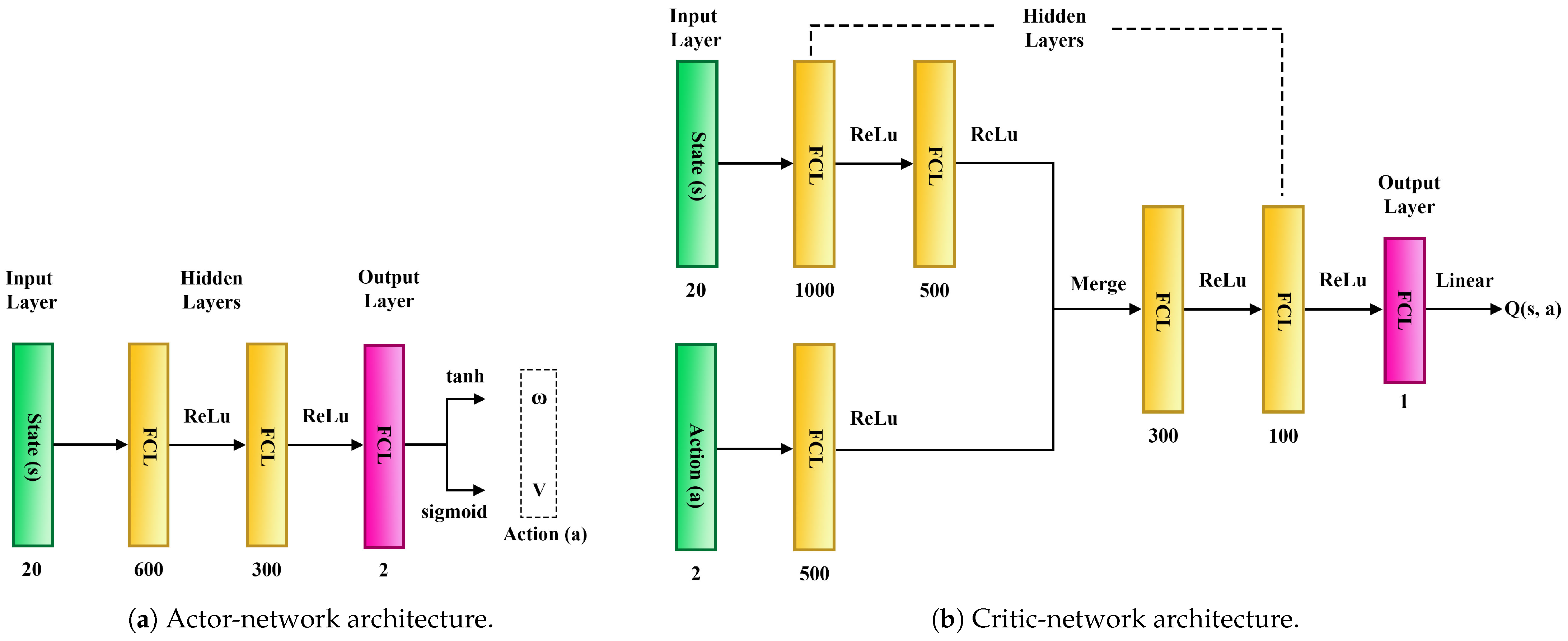
5.3. Navigation Agent

All the types of trainable agents we develop comprise two main components known as actor-network and critic-network. They are implemented with neural networks comprising fully connected layers (FCLs), and Figure 4 illustrates their architectures in detail. The network architectures we use for the simulation and physical experiment setups are similar. All the hidden nodes in every hidden layer are activated with the ReLu activation function [57], and weights are initialized with He initialization [58]. The actor-network consists of 193,502 trainable parameters, and the critic-network contains 823,701. The values we set for some critical hyper-parameters in each experiment setup are presented in Appendix B.
The actor-network (see Figure 4a) takes the current state as the input to produce the control signals as the output. The proximity sensor readings vector P = ( p 1 , p 2 , , p i , , p 16 ) , the angle between the heading and goal directions ( δ ), the distance to the goal (d), and the components of the linear velocity ( v x , v y ) are used to represent the state. Therefore, the state consists of 20 state variables. There are two outputs at the output layer to control the linear and angular velocities of the platform, and they represent the action. The control signal of the linear velocity (V) is calculated by a ‘ s i g m o i d ’ activation node, which limits output within the 0–1 range (the robot can move only in the forward direction). The ‘ t a n h ’ activation is used to produce the control signal for the angular velocity ( ω ), and it limits the output value between 1 and 1 as the robot can turn in both the right and left directions. The critic network takes state and action as the input and produces a linearly activated output representing the Q-value. The Adam optimizer optimizes both actor and critic networks.

5.4. Reward Function
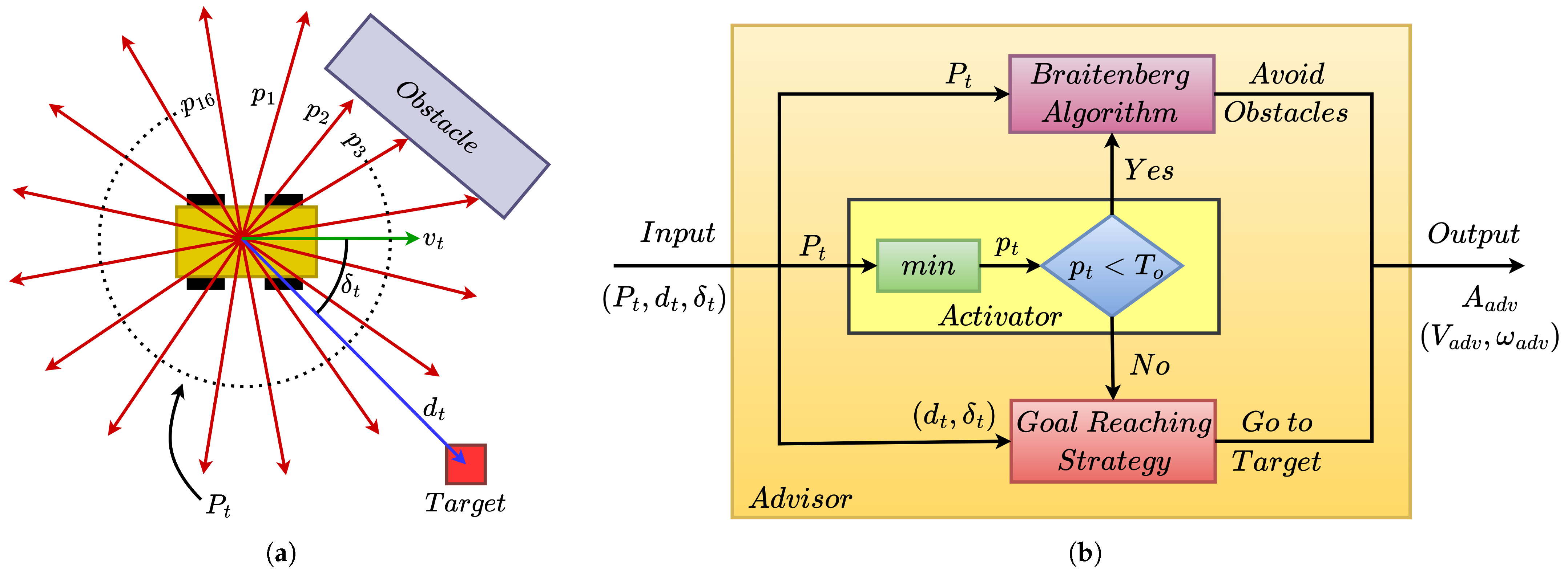
The reward function is mainly used to evaluate the action played by an RL agent at a given state, and a properly tuned reward always assists in converging the policy to optimal or sub-optimal faster. Therefore, we define a reward function that evaluates the actions executed in the terminal and intermediate states, as shown in Equation (8). Our experiments carry three terminal states for an episode: ‘goal’, ‘collision’, and ‘time out’. We call that the agent has reached the ‘goal’ state when the distance to the goal d t at a particular time step t is less than a constant threshold value T g ( T g is set to 0.15  m in all the experiments). If the P t is the proximity sensor reading array at time step t, we define the minimum obstacle distance at the same time step p t as p t = m i n ( P t ) . We call it a ‘collision’ if p t is less than a constant threshold T c ( T c = 0.1  m in the experiments). If the number of steps of an episode (h) exceeds the maximum step count of an episode ( h m a x ), it is considered a ‘time out.’ We assign a constant reward for the goal and collision terminal states, and the time out is not rewarded especially. We encourage reaching the goal with a large positive reward c 1 , and the collision is discouraged with a large negative reward c 2 ( c 2 > 0 ) . All the actions played at intermediate states are rewarded, considering whether the actions push the platform toward a goal or an obstacle. If the action reduces d, the agent is rewarded proportionally to the distance traveled towards the goal during the time step ( d t 1 d t ) . The agent is rewarded negatively if the agent moves toward an obstacle. Therefore, we add a reward component to the intermediate step proportional to the change in minimum proximity reading ( p t p t 1 ) . We combine those rewarding criteria to create the final reward function r, given in Equation (8). k 1 , and k 2 represent two positive proportional constants.
r = c 1 d t T g c 2 p t T c k 1 ( d t 1 d t ) + k 2 ( p t p t 1 ) O t h e r w i s e

5.5. Advisor

The advisor used in our experiments was created by combining a target-reaching controller and the classical Braitenberg navigation strategy [50] as illustrated in Figure 5b. The advisor activates the target-reaching controller if the agent finds no obstacle nearby (when p t = ( m i n ( P t ) ) exceeds a threshold value T o ). It produces linear and angular velocity control signals ( ω a d v and V a d v ) as functions of d t and δ t , as shown in Equations (9) and (10), where m 1 and m 2 are positive constants. Equation (9) produces an angular velocity control signal ( 1 < ω a d v < 1 ) that aligns the moving direction with the target direction. Also, Equation (10) generates the linear velocity control signal ( 0 < V a d v < 1 ) as a function of target distance d t . It sets the linear velocity closer to the maximum for large target distances and slows down the robot when it approaches the target position. Finally, the advisor’s control signals guide the platform toward the goal when no obstacle is nearby.
ω a d v = tanh ( m 1 δ t )
V a d v = [ 1 exp ( m 2 d t ) ]
The advisor activates the Braitenberg strategy-based obstacle-avoiding algorithm when it detects an obstacle nearby (if p t < T o ). The control signals are produced based on the closeness of the robot to the obstacles. They slow down the robot when it approaches an obstacle and moves away from the obstacles. However, the advisor we developed for our experiments cannot always successfully maneuver the platform to the goal position. This means that the advisor is capable of completing the given task to a certain extent, but it is not perfect. The pseudo-code of the advisor developed for goal-reaching with obstacle avoidance task and details of the implementation are presented in Appendix A.

6. Experiments and Results

The agents we test in our experiments are trained to perform the “goal-reaching with obstacle-avoiding” task. The experiments we carried out mainly focused on the following points.
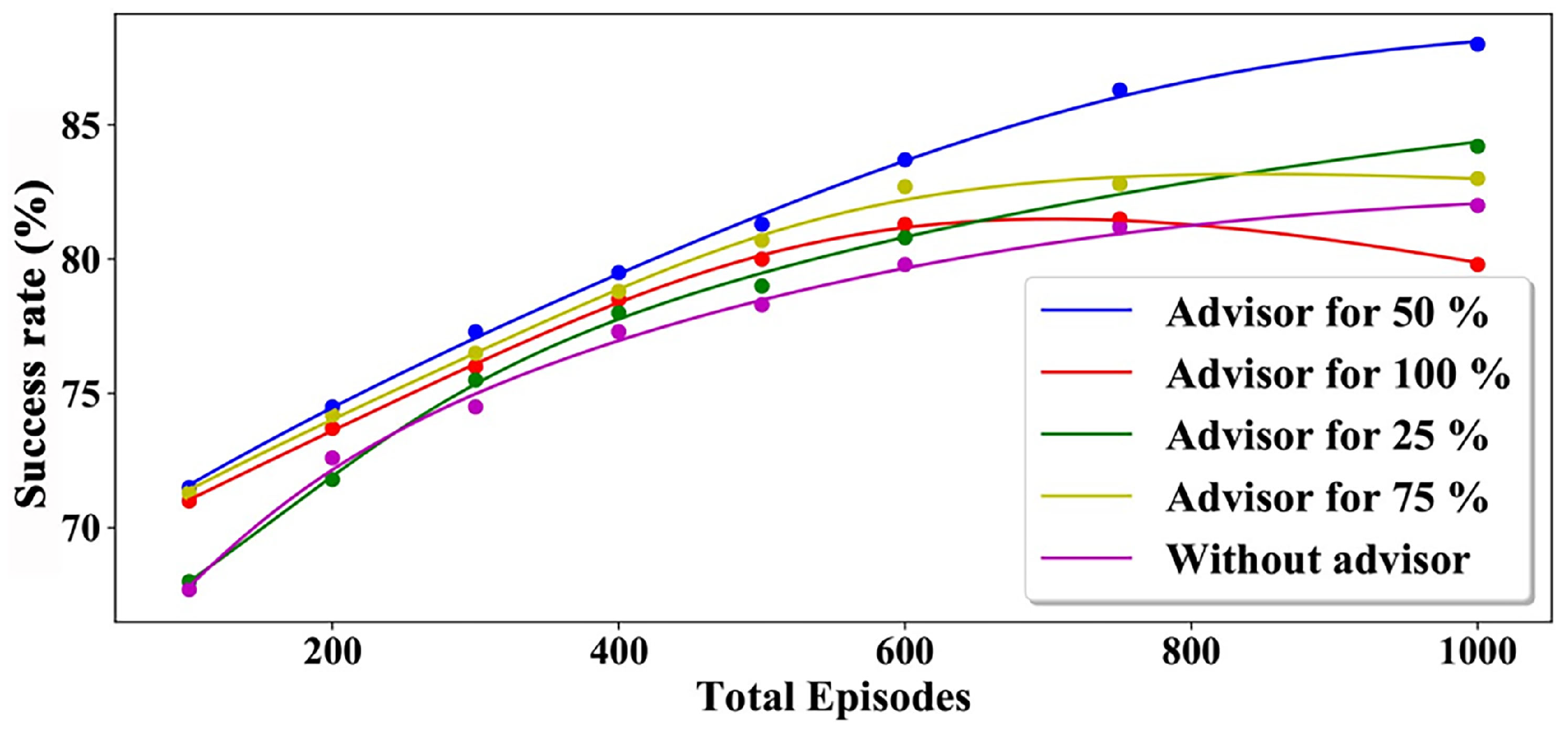
  • Checking the advisor’s influence on the training efficiency when the advisor is being used for the data collection and investigating the optimal way of employing the advisor in the data collection process.
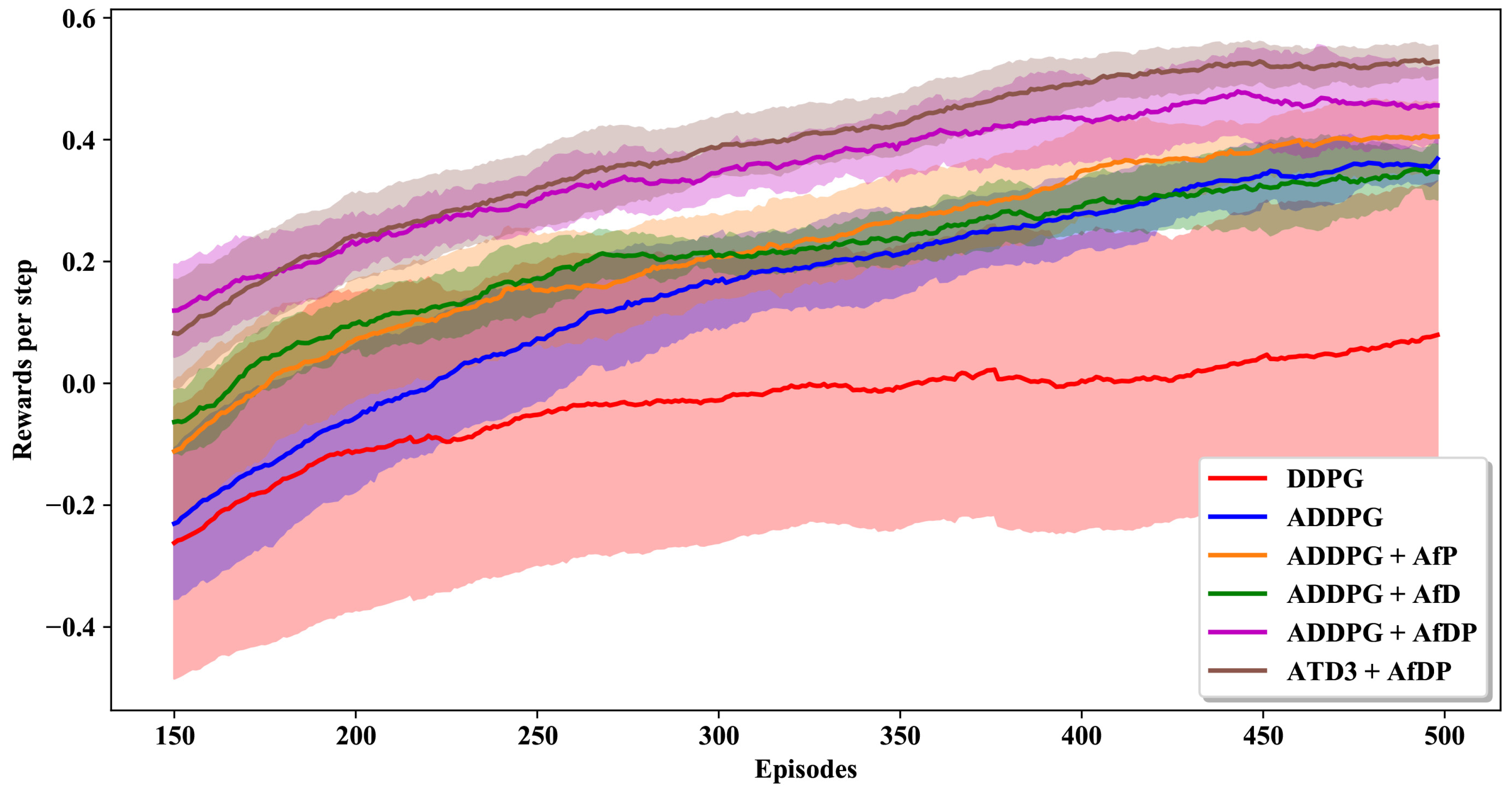
  • Checking the performance of the advisor-based architecture and comparing it against the other state-of-the-art methods.
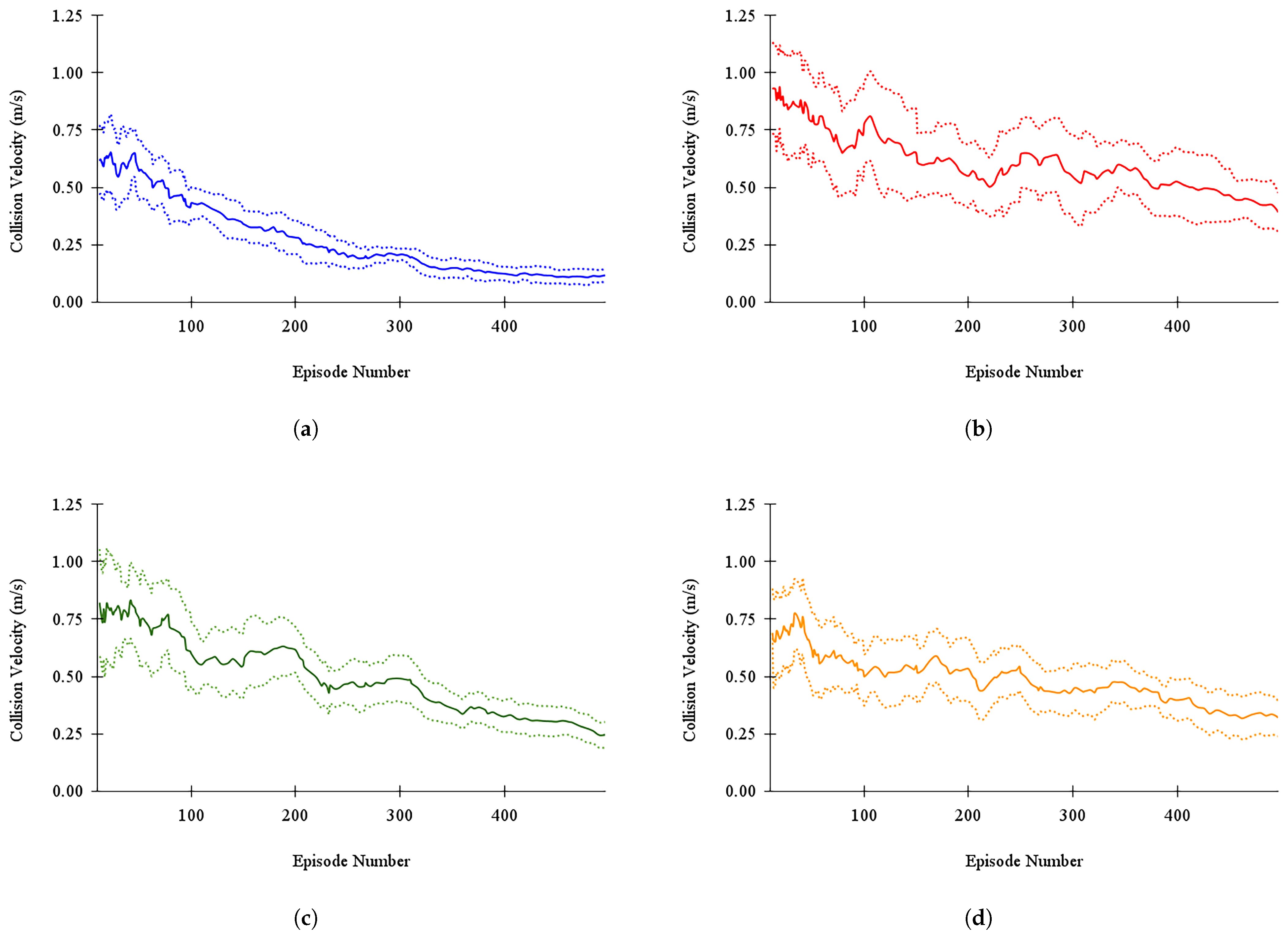
  • Checking the applicability of proposed advisor-based architecture on navigation tasks performed with real-world platforms assuring safe and efficient training.

6.1. Advisor’s Influence on Data Collection Process

We conduct a series of experiments on the simulation setup to investigate how the advisor influences training efficiency and the agent’s performance when the advisor contributes to the data collection process. As described earlier, the advisor can perform the assigned task to a certain level. We measure the performance of any trained agent or advisor in terms of the success rate, defined as the ratio of the number of successful episodes to the total number of testing episodes. An episode is counted as successful when it is ends with the ‘goal’ termination state. We test the advisor’s performances for 500 episodes on both training and validation environments, resulting in 53.6 % and 50.4 % success rates, respectively. To explore the best usage of the advisor, we train a group of agents that employ the advisor only for the data collection process by varying N T since it controls the advisor’s involvement. Each agent is implemented based on the advisor-based architecture that utilizes the advisor only for the data collection, and the ADDPG algorithm updates the policy. These agents are trained for 500 episodes in the training environment and tested for 100 episodes in both the training and validation environments. We record the success rate gained by the agents in both environments, and Figure 6 illustrates how the advisor’s involvement in data collection affects the final performance of the trained agents. It shows a similar success rate variation in both training and validating environments, indicating the trained agents are generalized for unseen environments.
When the advisor’s contribution to the data collection process increases (when N T increases), the advisor influences the agent to explore more within the knowledge limit of the advisor. Therefore, the agent’s predictions will be biased toward the advisor’s knowledge unless the advisor’s contribution is regulated properly. This behavior can be clearly seen in Figure 6. Since the advisor can perform the task to a certain level, we observe a performance improvement of the agents for the lower values of N T . The performance reaches a maximum when the advisor contributes nearly 50 % of the total number of episodes. However, a longer period of the advisor’s involvement in data collection has caused the agent to settle in a lower sub-optima state. This is because the agent has been forced by the advisor to limit the agent’s exploration within the range of the advisor’s knowledge.
To analyze the advisor’s influence on the performance of the trained agent further, we conduct another experiment that trains a group of agents by varying the total training episodes ( N t o t a l ). Then, the trained agents are tested for 100 episodes in the training environment, and the success rate of each agent is recorded. We repeat the same experiment while changing the advisor’s contribution, which is expressed as a percentage of N T with respect to N t o t a l . Figure 7 shows the performance variation of the trained agents against the total number of training episodes for different advisor contribution percentages.
We obtain the best performance when the advisor contributes 50 % of the total training episodes to the data collection (see the blue curve in Figure 7). The agent starts underperforming at higher total training episodes when the advisor’s contribution increases further (check the red and yellow curves in Figure 7). The agents with a longer advisor contribution move closer to the blue curve at the lower range of total training episodes since a higher contribution of an advisor is always favorable in the early stage of the learning process. However, the higher advisor contribution acts as a hurdle to a better exploration in the long run as the advisor is not perfect. When the number of training episodes increases, the agent performs better than the advisor at a certain level. The continuous involvement of the advisor beyond that level would be a weakness that limits the agent’s exploration. That is the reason for showing lower performance at higher total training episodes, even though the advisor contributes significantly. Relying on these results, we use 50 % as the advisor contribution in data collection for other experiments to make best use of the advisor.

6.2. Performance of Adviser-Based Architecture

We conduct another two experiments in a simulation setup to evaluate and compare the performance of advisor-based architecture by training various types of agents to perform the given navigation task. Also, we adapt the TD3 algorithm (referred to as ATD3) for use with advisor-based architecture and develop an agent that uses the advisor for both data collection and policy updating processes (check Appendix C for more information about the advisor-based ATD3 agent). We set the advisor’s contribution to 50 % (relying on the results in Section 6.1, we set 250 as N T ) for the agents in both experiments when the advisor contributes to the data collection. In the first experiment, we train all types of agents in the training environment for 500 episodes and test the success rate of the trained agents for 100 episodes in both training and testing environments. Also, we compare the performance of the trained agent against other training methods learning from demonstration (LfD) [59] and combined approach of model predictive control (MCP) and model-free learning [31]. Each agent type was trained and tested for six trials, and the average performance of each agent type is recorded in Table 1.
Table 1 clearly indicates that all the trained agents have surpassed the adviser’s performance after the training. Also, the advisor-based agent with the ATD3 algorithm (ATD3 + AfDP) outperforms all other algorithms by a significant margin. Moreover, agents that incorporate the advisor for training have demonstrated higher performances than most of the other agents, indicating that the proper involvement of an advisor in training is advantageous. However, the agent that incorporates the advisor for policy updating (ADDPG + AfP) shows better performance than the agent who uses the advisor only for data collection (ADDPG + AfD) as it does not enforce to select adviser’s suggestions during the policy updating. It allows the agent to select the most suitable set of actions based on the current knowledge of the agent. The agent who engages the advisor for policy updating and data collection outperforms all the other agent types, revealing the advantage of the regulated involvement of an advisor in the training process.
Figure 8 shows the episode-wise reward gained per step corresponding to each agent type, and it clearly illustrates how each agent type improves its performance over the progressing episodes. All advisor-based agent types have reached higher reward levels more quickly than the others, and the agents that employ the advisor for both data collection and policy updating have given the best performances. This exhibits how employing an advisor in data collection and policy updating expedites the learning process. Also, employing an advisor has reduced the standard deviation of the learning curve significantly. The agents that incorporate the advisor in the data collection have demonstrated the lowest standard deviations as the advisor highly restricts the agent’s exploration according to its perception. Since the agents are rewarded with large positive and negative rewards for goal-reaching and collision, respectively, having a higher standard deviation in the learning curve indicates experiencing many successes and failures during the training. However, the lower standard deviation and the higher reward gain of the agents who incorporate the advisor for both processes reflect that they experience more successes than collisions.
Apart from the higher reward gain with lower standard deviation, the collision velocity also provides a reliable safety measurement that can be used to assess the deployability of a learning algorithm run with a physical platform. Figure 9 clearly shows that the collision velocity and its standard deviation are significantly low when the advisor is involved in both data collection and policy updating compared to the others. The low collision velocity assures a low risk of damaging the physical platform at a collision against an obstacle. It makes the proposed architecture feasible to use for training real-world navigation tasks with a physical platform while assuring safe and expedited training.
Another observation of Figure 8 is a higher reward gain in the initial training phase by the advisor-based agents. Experiencing a higher reward gain is obvious when the advisor is used for policy updating as the advisor always assists in improving the existing policy towards a better policy. Also, exhibiting a higher reward gain in the initial training phase is explicable when the advisor is involved in the data collection as the advisor always guides the agent to explore better regions of the state and action spaces compared to the initial policy. However, the agent should experience a drop in the reward gain after the advisor’s termination unless the agent entirely captures the advisor’s knowledge before the termination. As we can see in Figure 8, the agents who use the advisor for data collection (check the green and magenta color graphs in Figure 8) do not indicate a significant drop in reward gain near N T (near the 250th episode).
E ( f r m a x ) = [ b N + 1 ϵ s t b 2 ( w 1 ) ]
The firing rate of the actor’s action f r a c t should be lower than the expected maximum firing rate if the agent cannot capture the advisor’s complete knowledge before the advisor’s termination. The actor’s firing rate is defined as the ratio between the number of steps that the actor’s action is selected for for the execution and the total number of steps in an episode. Suppose the actor learns from the advisor properly and improves its performance more than the advisor during the advisor’s involvement in data collection. In that case, there is a higher probability of obtaining a larger Q-value for the actor’s actions than the advisor’s. Then, the actor’s firing rate should be closer to the expected minimum firing rate E ( f r m a x ) . Equation (11) represents an estimation for E ( f r m a x ) , which is derived from Equation (1) (w is the window size of the moving average, and the derivation is presented in Appendix D). Figure 10 clearly shows that both agents that use the advisor for data collection demonstrate a similar firing rate to the expected maximum, proving that the advisor has been used effectively during the training.
In the next series of experiments, we change the number of training episodes of each agent type and record their success rate in both training and validation environments. Figure 11 summarizes the results of this experiment, and it illustrates the performance of each agent type in both training and validation environments. The performance variations of individual agents in both simulation environments are similar, which implies that each agent has learned generalized policies during the learning period. Also, once an adviser is employed in either data collection or policy updating, the training speed is boosted significantly and introduces a jump start for the reward gain at the initial stage. As a result, the agent incorporating the advisor for both the data collection and policy updating has shown the best performance compared to all the other agent types. Also, the ADDPG algorithm-based agents always show a significant improvement in the success rate compared to the original DDPG algorithm. Furthermore, employing an adviser with the ATD3 algorithm has produced the best results, indicating the capability of extending the method we developed to incorporate an advisor to the other variants of the DDPG algorithm and extracting the adviser’s knowledge effectively.

6.3. Performance with the Physical Platform

We use the physical setup described in Section 5.2 to investigate the applicability of the proposed advisor-based architecture in a real-world navigation task. According to the results we gained with simulation-based experiments, to obtain the best performance, we select the agent that uses the advisor for both data collection and policy updating processes with the advisor contribution of 50 % in the data collection. The algorithm we used to develop the advisor for the physical setup is similar to the simulation setup, and it can reach the goal position with a success rate of 32 % . We change the total number of training episodes corresponding to each agent and test the performance of each trained agent for 100 episodes in the same environment. The average performance of each agent type for different total training episodes is shown in Table 2, and a set of paths followed by the trained ATD3 + AfDP and DDPG agent in a few test trials is shown in Appendix E.
As we see in Table 2, the agent with the advisors outperforms the other agent types as we expected, establishing the applicability of the advisor-based architecture in real-world navigation tasks. Also, the advisor-based agent with the ATD3 algorithm (ATD3 + AfDP) has shown the best performance, similar to the experiments conducted with the simulation setup. Although the performances of the advisor-based agents do not reach a higher success rate similar to the simulation setup, the significant improvement over the other agent types reveals the advantage of incorporating an advisor for the training. This indicates that the proposed advisor-based architectures have expedited the training process to a significant level by transferring the previous knowledge through the advisor.
Furthermore, the collision velocities of the advisor and agents trained for 200 episodes are recorded during the testing phase. Table 3 shows the average collision velocities and their standard deviations. The table clearly indicates that the advisor’s involvement in training reduces the collision velocity significantly, assuring safe training compared to the other agents. The ATD3 agent incorporating the advisor for data collection and policy updating has achieved the lowest collision velocity, making it more suitable to train for navigation tasks with physical platforms.

7. Conclusions

In this research, we adapt the DDPG algorithm to incorporate previous knowledge into the training process of autonomous navigation agents to reduce the sample complexity. Also, we propose an architecture to facilitate using an advisor in policy updating and data collection processes to guarantee expedited learning. We present a method of using the advisor for data collection to train autonomous navigation agents to maneuver navigation platforms with a low risk of collision. We test the performance of the modified algorithm with the support of simulation and physical experimental setups and compare it to the existing state-of-the-art training approaches. The results gained with both simulation and physical experimental setups reveal that the agent that employs the advisor for both the data collection and policy updating process with a regulated advisor’s involvement in data collection guarantees the best performance in training. Also, the lower standard deviation introduced by the advisor to the learning curve and lower collision velocity guarantees safe training with minimum damages, which is highly favorable in training an agent that controls a physical platform.
Finding the optimal way of employing the advisor is highly challenging as it depends on numerous factors, such as on the nature of the task and on the advisor’s performance. Therefore, it is necessary to develop a generalized method for regulating the advisor’s contribution across various navigation tasks as our future goal. Furthermore, it is important to acknowledge that the advisor-based architecture may not lead the agent to acquire the optimal policy for the given task. Therefore, it is interesting to find methods to develop a productive advisor for a given task that guarantees guidance toward the optimal policy for a given navigation task. A detailed analysis of the influence of ill-posed advisors on training will be useful in quantifying the overall efficiency of the proposed method. Also, employing multiple advisors, each specialized in various sub-tasks, is worth investigating as it is a much more convenient approach to addressing complex navigation tasks than developing a single advisor.

Author Contributions

Conceptualization, R.D.W., D.T. and J.S.; Methodology, R.D.W., M.K.V. and A.X.; Software, R.D.W.; Formal analysis, R.D.W.; Investigation, D.T.; Writing—original draft, D.T., M.K.V., A.X. and S.F.; Writing—review and editing, M.K.V. and J.S.; Visualization, A.X., S.F. and J.S.; Supervision, S.F. and J.S. All authors have read and agreed to the published version of the manuscript.

Funding

This research is funded by the University of Moratuwa and CodeGen International (Pvt) Ltd under the Q-Bits Scholar grant.

Data Availability Statement

Not applicable.

Acknowledgments

We thank Sanath Jayasena and Ranga Rodrigo for arranging insightful discussions supporting this work.

Conflicts of Interest

The authors declare no conflict of interest.

Abbreviations

    The following abbreviations are used in this manuscript:
RLReinforcement learning
DQNDeep-Q-network
DDPGDeep deterministic policy gradient
TD3Twin-delayed DDPG
SLAMSimultaneous localisation and mapping
IntRLInteractive reinforcement learning
ILIntegrating imitation learning
BADGRBerkeley autonomous driving ground robot
V-repVirtual robot experimentation platform
APIApplication programming interface
RGBRed green blue
PCPersonal computer
GPUGraphical processing unit
CPUCentral processing unit
RAMRandom access memory
FCLFully connected layers
ADDPGAdapted deep deterministic policy gradient
ATD3Adapted twin-delayed DDPG
LfDLearning from demonstration
MCPModel predictive control
AfDAdvisor for data collection
AfPAdvisor for policy updating
AfDPAdvisor for both data collection and policy updating

Appendix A. Implementation of the Advisor

Algorithm A1 describes the method we used to develop the advisor employed in our experiments. Based on prior knowledge, the advisor aims to produce angular and linear velocity control signals ( ω a d v and V a d v ) relevant to the given task. It has two main functions responsible for generating control signals for target reaching and obstacle avoidance. Each time step in a running episode; it measures 16 ( N s e n = 16 ) proximity sensor values P, target angle δ , and target distance d. Depending on the minimum proximity sensor measurement p m i n , it activates the relevant function. The threshold value for obstacle avoidance T o represents the limit for the p m i n to decide whether an obstacle is nearby. T o is set to 0.5 m and 0.6 m for the experiments we carried out with the simulation and physical setups, respectively. If  p m i n < T o , it identifies that the robot has moved closer to an obstacle and activates the Braitenberg strategy-based obstacle-avoiding function. It calculates the control signals based on the normalized closeness of the sensor readings d e t (see step 19 of the Algorithm A1). Otherwise, the advisor produces the control signals to guide the robot toward the target position based on δ and d. Additionally, the other parameters in the algorithm are set to the values given in Table A1 for both simulation and physical setups.
The advisor uses only the front eight proximity sensor readings ( p 1 , , p 8 ) to make the calculations as the experiments are designed to move the robot in the forward direction only. Therefore, the last sets of elements of b R and b L are set to 0 to eliminate the effect of rear sensor readings.
Table A1. Values of the parameters in advisor algorithm.
ParameterValue
No detect distance ( d n d )0.6 m
Maximum detect distance ( d d m a x )0.2 m
Left Braitenberg array ( b L ) [ 0.1 , 0.2 , 0.3 , 0.4 , 0.5 , 0.6 , 0.7 , 0.8 , 0 , 0 , 0 , 0 , 0 , 0 , 0 , 0 ]
Right Braitenberg array ( b R ) [ 0.8 , 0.7 , 0.6 , 0.5 , 0.4 , 0.3 , 0.2 , 0.1 , 0 , 0 , 0 , 0 , 0 , 0 , 0 , 0 ]
Maximum linear velocity ( V m a x )1.0 ms 1
m 1 1.0
m 2 5.0
m 3 1.0
Algorithm A1 Advisor for goal reaching with obstacle avoiding
  1:
Initialize number of proximity sensors n s e n
  2:
Initialize no detect distance d n d
  3:
Initialize maximum detect distance d d m a x
  4:
Initialize the detect array to zeros d e t n s e n × [ 0 ]
  5:
Initialize left and right Braitenberg arrays,
       b R [ r 1 , r 2 , , r n s e n ]
       b L [ l 1 , l 2 , , l n s e n ]
  6:
Initialize maximum linear velocity V m a x
  7:
while episode is not terminated do
  8:
      Obtain input sensor readings
            Obtain proximity sensor readings P                                    ▹ P = [ p 1 , p 2 , , p n s e n ]
            Obtain current target distance d and target angle δ
  9:
      Obtain proximity sensor reading p m i n m i n ( P )
10:
      if  p m i n > T o  then                                                                    ▹ Activate target reaching
11:
            ω a d v tanh ( m 1 δ )                                  ▹ m 1 is a proportional constant ( m 1 > 0 )
12:
            V a d v [ 1 exp ( m 2 d ) ]                     ▹ m 2 is a proportional constant ( m 2 > 0 )
13:
      else                                                         ▹ Activate the Braitenberg obstacles avoiding
14:
            for  1 : i : n s e n  do
15:
               if  p [ i ] < d n d  then
16:
                   if  p [ i ] < d d m a x  then
17:
                        p [ i ] d d m a x
18:
                    d e t [ i ] 1.0 [ p [ i ] d d m a x d n d d d m a x ]                                                         ▹ 0 d e t [ i ] 1
19:
               else
20:
                    d e t [ i ] 0
21:
            V a d v V m a x + 1 2 [ b R + b L ] · d e t
22:
            ω a d v m 3 2 [ b L b R ] · d e t                                                                               ▹ m 3 > 0
23:
       ω a d v c l i p ( ω a d v , 1.0 , 1.0 )
24:
       V a d v c l i p ( V a d v , 0.0 , 1.0 )

Appendix B. Parameter Values Used in the Implementation of the Advisor-Based Navigation Agent

Table A2. Values set for hyper-parameters of ADDPG-based agents in simulation and physical setup.
Hyper-ParameterSimulation SetupPhysical Setup
Memory replay buffer size100,00050,000
Batch size (n)1000500
Discount rate ( γ ) 0.9 0.9
Soft updating rate ( τ ) 0.1 0.1
Policy updating rate ( β ) 0.01 0.01
Actor learning rate ( α a c t o r ) 1 × 10 5 1 × 10 4
Critic learning rate ( α c r i t i c ) 1 × 10 3 1 × 10 3
Starting advisor selection probability ( ϵ s t ) 0.85 0.9
Selection probability rate (b) 0.15 0.001
Maximum number of steps per episode ( h m a x )300150
Table A3. Values of the parameters in the reward function used for experimental and physical setups.
ParameterValue
Threshold of target distance for goal reaching T g 0.15 m
Threshold of the minimum proximity reading for collision T c 0.1 m
c 1 10.0
c 2 10.0
k 1 5.0
k 2 5.0
Table A4. Values set for hyper-parameters specified only for ATD3 base agents.
Hyper-ParameterSimulation SetupPhysical Setup
μ 00
σ ¯ 0.1 0.05
c 0.2 0.1
d43
Note—Values of the parameters common for ADDPG and ATD3 algorithms are similar to the values present in Table A2.

Appendix C. Adapt the TD3 Algorithm to Incorporate an Advisor

Algorithm A2 Data collection with an advisor
  1:
Initialize total number of training episodes N t o t a l
  2:
Initialize terminal episode number of the advisor N T
  3:
Initialize advisor’s starting execution probability ϵ s t
  4:
for  1 : N : N t o t a l   do
  5:
    Load the policy π ( s ; ϕ ) from the policy updating
    process
  6:
    Load the Q-value functions Q 1 ( s , a ; θ 1 ) and
     Q 1 ( s , a ; θ 2 ) (critic-networks) from the policy
    updating process
  7:
    while episode is not terminated do
  8:
        Observe current state s
  9:
        Calculate advisor’s action a a d v f ( s )
10:
        Calculate actor’s action a a c t π ( s ; ϕ )
11:
         Q a c t m i n ( Q 1 ( s , a a c t ; θ 1 ) , Q 2 ( s , a a c t ; θ 2 ) )
12:
         Q a d v m i n ( Q 1 ( s , a a d v ; θ 1 ) , Q 2 ( s , a a d v ; θ 2 ) )
13:
        Calculate advisor’s execution probability ϵ using
        Equation (A1)
14:
        With probability ϵ , a a a d v or otherwise,
         a a a c t
15:
         a a + n o i s e
16:
        Execute action a
17:
        Observe next state s and reward r
18:
        Store ( s , a , s , r ) in the memory replay buffer
ϵ = 1 ( Q a c t Q a d v ) ( N N T ) ϵ s t b N ( Q a c t > Q a d v ) ( N N T ) 0 N > N T
Algorithm A3 Policy updating with an advisor
  1:
Create actor-network π ( s ; ϕ ) and target actor-network π T ( s ; ϕ T )
  2:
Create critic-networks Q 1 ( s , a ; θ 1 ) and Q 2 ( s , a ; θ 2 )
  3:
Create target critic-networks Q 1 T ( s , a ; θ 1 T ) and Q 2 T ( s , a ; θ 2 T )
  4:
Initialize actor and critic networks parameters ( ϕ , θ 1 and θ 2 ) with He initialization
  5:
Initialize target networks’ parameters;
     ϕ T ϕ
     θ 1 T θ 1
     θ 2 T θ 2
  6:
Initialize time-step t to 0
  7:
repeat:
  8:
     t t + 1
  9:
     Sample a batch of experiences
     B = < S , A , A a d v , R , S > randomly from memory
     replay buffer with the size of n
10:
     Δ A c l i p ( N ( μ , σ ¯ ) , c , c )
11:
     A π T ( S ; ϕ T ) + Δ A
12:
     Q ^ R + γ m i n ( Q 1 T ( S , A ; θ 1 T ) , Q 2 T ( S , A ; θ 2 T ) )
13:
     Update θ 1 by minimizing the loss function L Q 1
            L Q 1 = 1 n Σ [ Q ^ Q 1 ( S , A ; θ 1 ) ] 2
14:
     Update θ 2 by minimizing the loss function L Q 1
            L Q 1 = 1 n Σ [ Q ^ Q 2 ( S , A ; θ 2 ) ] 2
15:
     if t mod d then
16:
            A a c t π ( S ; ϕ )
17:
            A ^ A a c t + β A Q 1 ( S , A a c t ; θ )
18:
            for  1 : i : n  do
19:
                 if  Q 1 ( s i , a a d v i ; θ ) > Q 1 ( s i , a ^ i ; θ )  then
20:
                      a ^ i a a d v i
21:
            Update ϕ by minimizing the loss function L π
                 L π = 1 n Σ [ A ^ π ( S ; ϕ ) ] 2
22:
            Update target networks parameters
                 ϕ T τ ϕ + ( 1 τ ) ϕ T
                 θ 1 T τ θ 1 + ( 1 τ ) θ 1 T
                 θ 2 T τ θ 2 + ( 1 τ ) θ 2 T
23:
     Store all the networks

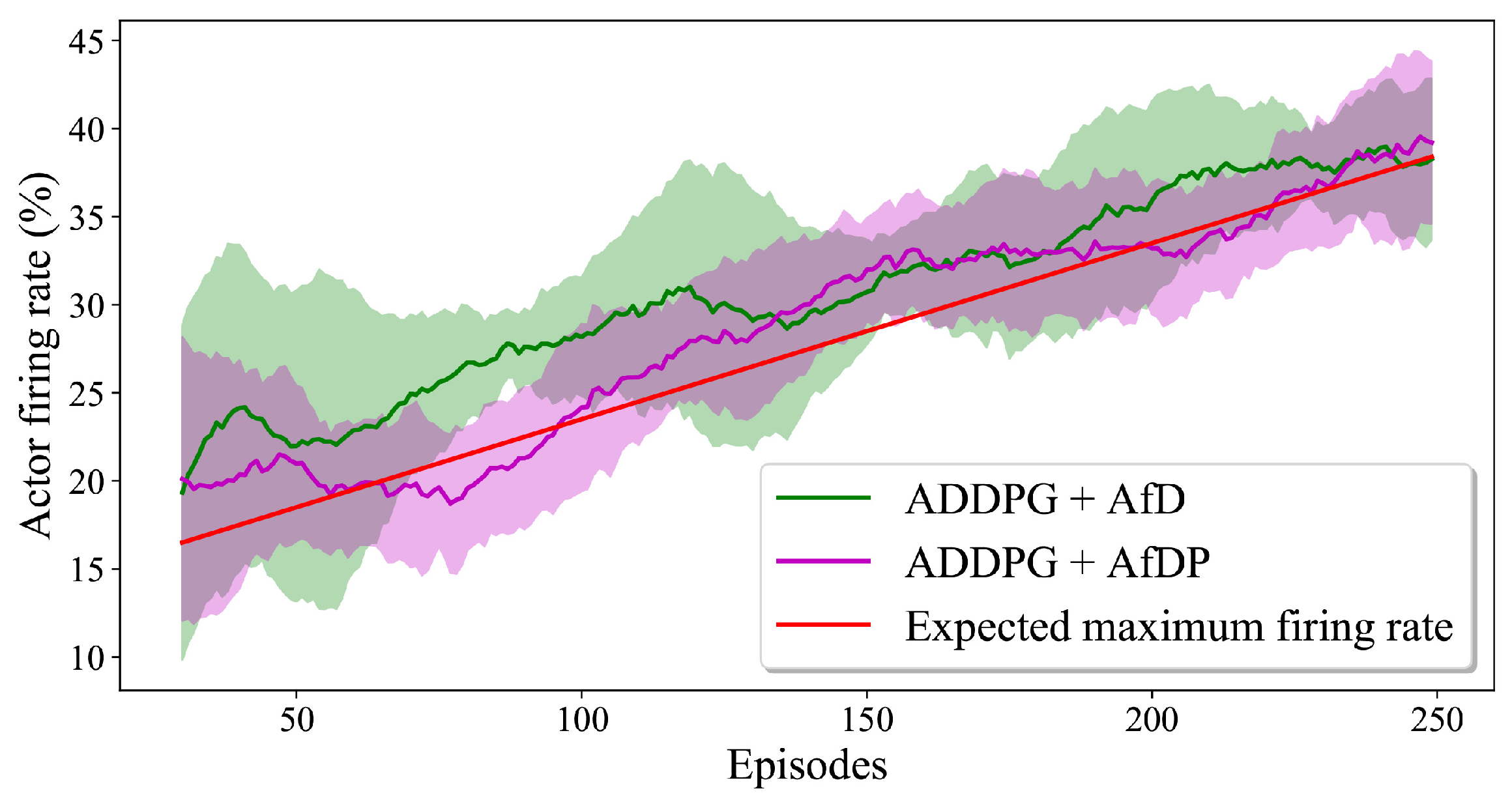
Appendix D. Actor’s Expected Maximum Firing Rate

By considering Equation (1), we can find the actor’s execution probability ϵ a c t before the advisor’s termination ( N < N T ) as follows:
ϵ a c t = 1 ϵ a d v ϵ a c t = 0 ( Q a c t Q a d v ) ( N N T ) b N + 1 ϵ s t ( Q a c t > Q a d v ) ( N N T )
The expected actor’s firing rate E ( f r a c t ) at the Nth episode can be expressed as
E ( f r a c t ) = 1 h m a x E ( h a c t ) h a c t Number of steps fired by the actor in an episode = 1 h m a x h = 1 h m a x ϵ a c t h Step count in an episode
Therefore, we can find an upper bound for the expected actor’s firing rate E ( f r u b ) at the Nth episode if Q a c t > Q a d v in every step of an episode (when the actor learned a better policy than the advisor).
E ( f r u b ) = 1 h m a x h = 1 h m a x [ b N + 1 ϵ s t ] ) = 1 h m a x [ b N + 1 ϵ s t ] h m a x = b N + 1 ϵ s t
The moving average of the expected maximum firing rate E ( f r m a x ) at the N t h episode can be derived as follows:
E ( f r m a x ) = 1 w i = N w + 1 N E ( f r u b ) i Episode count = 1 w i = N w + 1 N [ b N + 1 ϵ s t ] = 1 w [ w 2 ( N + N w + 1 ) + w ( 1 ϵ s t ) ] = N b + 1 ϵ s t b 2 ( w 1 )

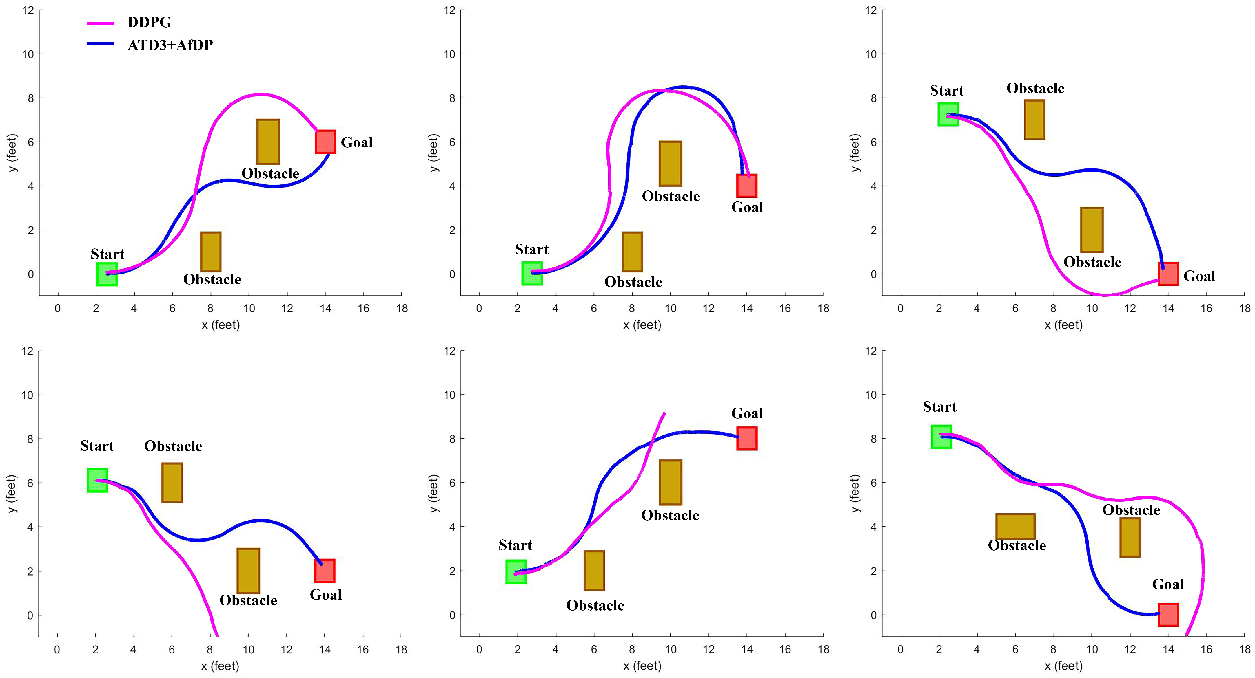
Appendix E. Paths Followed by the Trained Agents with and without the Advisor

Figure A1. Paths followed by the trained ATD3+AfDP and DDPG agent in six trials. The blue line represents the path followed by the ATD3+AfDP agent, and the magenta line shows the DDPG agent’s path.
Robotics 12 00133 g0a1

References

  1. Yang, Y.; Wang, J. An overview of multi-agent reinforcement learning from game theoretical perspective. arXiv 2020, arXiv:2011.00583. [Google Scholar]
  2. Lample, G.; Chaplot, D.S. Playing FPS games with deep reinforcement learning. In Proceedings of the AAAI Conference on Artificial Intelligence, San Francisco, CA, USA, 4–9 February 2017; Volume 31. [Google Scholar]
  3. Mnih, V.; Kavukcuoglu, K.; Silver, D.; Rusu, A.A.; Veness, J.; Bellemare, M.G.; Graves, A.; Riedmiller, M.; Fidjeland, A.K.; Ostrovski, G.; et al. Human-level control through deep reinforcement learning. Nature 2015, 518, 529–533. [Google Scholar] [CrossRef] [PubMed]
  4. Afsar, M.M.; Crump, T.; Far, B. Reinforcement learning based recommender systems: A survey. ACM Comput. Surv. 2022, 55, 1–38. [Google Scholar] [CrossRef]
  5. Kober, J.; Bagnell, J.A.; Peters, J. Reinforcement learning in robotics: A survey. Int. J. Robot. Res. 2013, 32, 1238–1274. [Google Scholar] [CrossRef]
  6. Ni, P.; Zhang, W.; Zhang, H.; Cao, Q. Learning efficient push and grasp policy in a tote box from simulation. Adv. Robot. 2020, 34, 873–887. [Google Scholar] [CrossRef]
  7. Shi, J.; Dear, T.; Kelly, S.D. Deep reinforcement learning for snake robot locomotion. IFAC-PapersOnLine 2020, 53, 9688–9695. [Google Scholar] [CrossRef]
  8. Wiedemann, T.; Vlaicu, C.; Josifovski, J.; Viseras, A. Robotic information gathering with reinforcement learning assisted by domain knowledge: An application to gas source localization. IEEE Access 2021, 9, 13159–13172. [Google Scholar] [CrossRef]
  9. Martinez, J.F.; Ipek, E. Dynamic multicore resource management: A machine learning approach. IEEE Micro 2009, 29, 8–17. [Google Scholar] [CrossRef]
  10. Ipek, E.; Mutlu, O.; Martínez, J.F.; Caruana, R. Self-optimizing memory controllers: A reinforcement learning approach. ACM SIGARCH Comput. Archit. News 2008, 36, 39–50. [Google Scholar] [CrossRef]
  11. Wang, C.; Wang, J.; Shen, Y.; Zhang, X. Autonomous navigation of UAVs in large-scale complex environments: A deep reinforcement learning approach. IEEE Trans. Veh. Technol. 2019, 68, 2124–2136. [Google Scholar] [CrossRef]
  12. Blum, T.; Paillet, G.; Masawat, W.; Yoshida, K. SegVisRL: Development of a robot’s neural visuomotor and planning system for lunar exploration. Adv. Robot. 2021, 35, 1359–1373. [Google Scholar] [CrossRef]
  13. Xue, W.; Liu, P.; Miao, R.; Gong, Z.; Wen, F.; Ying, R. Navigation system with SLAM-based trajectory topological map and reinforcement learning-based local planner. Adv. Robot. 2021, 35, 939–960. [Google Scholar] [CrossRef]
  14. Silver, D.; Huang, A.; Maddison, C.J.; Guez, A.; Sifre, L.; Van Den Driessche, G.; Schrittwieser, J.; Antonoglou, I.; Panneershelvam, V.; Lanctot, M.; et al. Mastering the game of Go with deep neural networks and tree search. Nature 2016, 529, 484–489. [Google Scholar] [CrossRef]
  15. Lillicrap, T.P.; Hunt, J.J.; Pritzel, A.; Heess, N.; Erez, T.; Tassa, Y.; Silver, D.; Wierstra, D. Continuous control with deep reinforcement learning. In Proceedings of the International Conference on Learning Representations (ICLR), San Juan, PR, USA, 2–4 May 2016. [Google Scholar]
  16. Fujimoto, S.; Hoof, H.; Meger, D. Addressing function approximation error in actor–critic methods. In Proceedings of the International Conference on Machine Learning, PMLR, Stockholm, Sweden, 10–15 July 2018; pp. 1587–1596. [Google Scholar]
  17. Hasselt, H. Double Q-learning. In Proceedings of the Advances in Neural Information Processing Systems (NeurIPS), Vancouver, BC, Canada, 6–8 December 2010. [Google Scholar]
  18. Liu, R.; Nageotte, F.; Zanne, P.; de Mathelin, M.; Dresp-Langley, B. Deep reinforcement learning for the control of robotic manipulation: A focussed mini-review. Robotics 2021, 10, 22. [Google Scholar] [CrossRef]
  19. Kormushev, P.; Calinon, S.; Caldwell, D.G. Reinforcement learning in robotics: Applications and real-world challenges. Robotics 2013, 2, 122–148. [Google Scholar] [CrossRef]
  20. Wijesinghe, R.; Vithanage, K.; Tissera, D.; Xavier, A.; Fernando, S.; Samarawickrama, J. Transferring Domain Knowledge with an Adviser in Continuous Tasks. In Pacific-Asia Conference on Knowledge Discovery and Data Mining; Springer: Cham, Switzerland, 2021; pp. 194–205. [Google Scholar]
  21. Sutton, R.S.; Barto, A.G. Introduction to Reinforcement Learning; MIT Press: Cambridge, UK, 1998; Volume 2. [Google Scholar]
  22. Silver, D.; Lever, G.; Heess, N.; Degris, T.; Wierstra, D.; Riedmiller, M. Deterministic policy gradient algorithms. In Proceedings of the International Conference Machine Learning (ICML), Beijing, China, 21–26 June 2014. [Google Scholar]
  23. Peters, J.; Schaal, S. Natural actor–critic. Neurocomputing 2008, 71, 1180–1190. [Google Scholar] [CrossRef]
  24. Van Hasselt, H.; Guez, A.; Silver, D. Deep reinforcement learning with double q-learning. In Proceedings of the AAAI Conference on Artificial Intelligence, Phoenix, AZ, USA, 12–17 February 2016; Volume 30. [Google Scholar]
  25. Haarnoja, T.; Zhou, A.; Abbeel, P.; Levine, S. Soft actor–critic: Off-policy maximum entropy deep reinforcement learning with a stochastic actor. arXiv 2018, arXiv:1801.01290. [Google Scholar]
  26. Gu, S.; Lillicrap, T.; Sutskever, I.; Levine, S. Continuous deep q-learning with model-based acceleration. In Proceedings of the International Conference on Machine Learning, New York, NY, USA, 19–21 June 2016; pp. 2829–2838. [Google Scholar]
  27. Dadvar, M.; Nayyar, R.K.; Srivastava, S. Learning Dynamic Abstract Representations for Sample-Efficient Reinforcement Learning. arXiv 2022, arXiv:2210.01955. [Google Scholar]
  28. Wen, S.; Zhao, Y.; Yuan, X.; Wang, Z.; Zhang, D.; Manfredi, L. Path planning for active SLAM based on deep reinforcement learning under unknown environments. Intell. Serv. Robot. 2020, 13, 263–272. [Google Scholar] [CrossRef]
  29. Tai, L.; Paolo, G.; Liu, M. Virtual-to-real deep reinforcement learning: Continuous control of mobile robots for mapless navigation. In Proceedings of the International Conference on Intelligent Robots and Systems (IROS), Vancouver, BC, Canada, 24–28 September 2017; pp. 31–36. [Google Scholar]
  30. Kahn, G.; Villaflor, A.; Ding, B.; Abbeel, P.; Levine, S. Self-supervised deep reinforcement learning with generalized computation graphs for robot navigation. In Proceedings of the IEEE International Conference on Robotics and Automation (ICRA), Brisbane, Australia, 21–25 May 2018; pp. 1–8. [Google Scholar]
  31. Nagabandi, A.; Kahn, G.; Fearing, R.S.; Levine, S. Neural network dynamics for model-based deep reinforcement learning with model-free fine-tuning. In Proceedings of the IEEE International Conference on Robotics and Automation (ICRA), Brisbane, Australia, 21–25 May 2018; pp. 7559–7566. [Google Scholar]
  32. Arzate Cruz, C.; Igarashi, T. A survey on interactive reinforcement learning: Design principles and open challenges. In Proceedings of the 2020 ACM Designing Interactive Systems Conference, Virtual, 6–10 July 2020; pp. 1195–1209. [Google Scholar]
  33. Lin, J.; Ma, Z.; Gomez, R.; Nakamura, K.; He, B.; Li, G. A review on interactive reinforcement learning from human social feedback. IEEE Access 2020, 8, 120757–120765. [Google Scholar] [CrossRef]
  34. Bignold, A.; Cruz, F.; Dazeley, R.; Vamplew, P.; Foale, C. Human engagement providing evaluative and informative advice for interactive reinforcement learning. Neural Comput. Appl. 2022, 35, 18215–18230. [Google Scholar] [CrossRef]
  35. Millan-Arias, C.C.; Fernandes, B.J.; Cruz, F.; Dazeley, R.; Fernandes, S. A robust approach for continuous interactive actor–critic algorithms. IEEE Access 2021, 9, 104242–104260. [Google Scholar] [CrossRef]
  36. Bignold, A.; Cruz, F.; Dazeley, R.; Vamplew, P.; Foale, C. Persistent rule-based interactive reinforcement learning. Neural Comput. Appl. 2021, 1–18. [Google Scholar] [CrossRef]
  37. Zhang, J.; Springenberg, J.T.; Boedecker, J.; Burgard, W. Deep reinforcement learning with successor features for navigation across similar environments. In Proceedings of the IEEE/RSJ International Conference on Intelligent Robots and Systems (IROS 2017), Vancouver, BC, Canada, 24–28 September 2017; pp. 2371–2378. [Google Scholar]
  38. Parisotto, E.; Ba, J.L.; Salakhutdinov, R. Actor-mimic: Deep multitask and transfer reinforcement learning. arXiv 2015, arXiv:1511.06342. [Google Scholar]
  39. Ross, S.; Gordon, G.; Bagnell, D. A reduction of imitation learning and structured prediction to no-regret online learning. In Proceedings of the Fourteenth International Conference on Artificial Intelligence and Statistics, Lauderdale, FL, USA, 11–13 April 2011; pp. 627–635. [Google Scholar]
  40. Amini, A.; Gilitschenski, I.; Phillips, J.; Moseyko, J.; Banerjee, R.; Karaman, S.; Rus, D. Learning robust control policies for end-to-end autonomous driving from data-driven simulation. IEEE Robot. Autom. Lett. 2020, 5, 1143–1150. [Google Scholar] [CrossRef]
  41. Kabzan, J.; Hewing, L.; Liniger, A.; Zeilinger, M.N. Learning-based model predictive control for autonomous racing. IEEE Robot. Autom. Lett. 2019, 4, 3363–3370. [Google Scholar] [CrossRef]
  42. Taylor, M.E.; Kuhlmann, G.; Stone, P. Autonomous transfer for reinforcement learning. In Proceedings of the International Joint Conference on Autonomous Agents and Multiagent Systems (AAMAS 2008)-Volume 1, Estoril, Portugal, 12–16 May 2008; pp. 283–290. [Google Scholar]
  43. Kinose, A.; Taniguchi, T. Integration of imitation learning using GAIL and reinforcement learning using task-achievement rewards via probabilistic graphical model. Adv. Robot. 2020, 34, 1055–1067. [Google Scholar] [CrossRef]
  44. Qian, K.; Liu, H.; Valls Miro, J.; Jing, X.; Zhou, B. Hierarchical and parameterized learning of pick-and-place manipulation from under-specified human demonstrations. Adv. Robot. 2020, 34, 858–872. [Google Scholar] [CrossRef]
  45. Sosa-Ceron, A.D.; Gonzalez-Hernandez, H.G.; Reyes-Avendaño, J.A. Learning from Demonstrations in Human–Robot Collaborative Scenarios: A Survey. Robotics 2022, 11, 126. [Google Scholar] [CrossRef]
  46. Oh, J.; Guo, Y.; Singh, S.; Lee, H. Self-imitation learning. arXiv 2018, arXiv:1806.05635. [Google Scholar]
  47. Nair, A.; McGrew, B.; Andrychowicz, M.; Zaremba, W.; Abbeel, P. Overcoming exploration in reinforcement learning with demonstrations. In Proceedings of the IEEE International Conference on Robotics and Automation (ICRA 2018), Brisbane, Australia, 21–25 May 2018; pp. 6292–6299. [Google Scholar]
  48. Hester, T.; Vecerik, M.; Pietquin, O.; Lanctot, M.; Schaul, T.; Piot, B.; Horgan, D.; Quan, J.; Sendonaris, A.; Osband, I.; et al. Deep q-learning from demonstrations. In Proceedings of the Thirty-Second AAAI Conference on Artificial Intelligence, New Orleans, LA, USA, 2–7 February 2018. [Google Scholar]
  49. Kahn, G.; Abbeel, P.; Levine, S. Badgr: An autonomous self-supervised learning-based navigation system. IEEE Robot. Autom. Lett. 2021, 6, 1312–1319. [Google Scholar] [CrossRef]
  50. Yang, X.; Patel, R.V.; Moallem, M. A fuzzy–braitenberg navigation strategy for differential drive mobile robots. J. Intell. Robot. Syst. 2006, 47, 101–124. [Google Scholar] [CrossRef]
  51. Konda, V.R.; Tsitsiklis, J.N. Actor–critic algorithms. In Proceedings of the Advances in Neural Information Processing Systems, Denver, CO, USA, 4–9 December 2000; pp. 1008–1014. [Google Scholar]
  52. Mnih, V.; Badia, A.P.; Mirza, M.; Graves, A.; Lillicrap, T.; Harley, T.; Silver, D.; Kavukcuoglu, K. Asynchronous methods for deep reinforcement learning. In Proceedings of the International Conference on Machine Learning (ICML), New York, NY, USA, 19–24 June 2016; pp. 1928–1937. [Google Scholar]
  53. Gu, S.; Holly, E.; Lillicrap, T.; Levine, S. Deep reinforcement learning for robotic manipulation with asynchronous off-policy updates. In Proceedings of the International Conference on Robotics and Automation (ICRA), Singapore, 29 May–3 June 2017; pp. 3389–3396. [Google Scholar]
  54. Uhlenbeck, G.E.; Ornstein, L.S. On the theory of the Brownian motion. Phys. Rev. 1930, 36, 823. [Google Scholar] [CrossRef]
  55. Rohmer, E.; Singh, S.P.; Freese, M. V-REP: A versatile and scalable robot simulation framework. In Proceedings of the International Conference Intelligent Robots and Systems (IROS), Tokyo, Japan, 3–7 December 2013; pp. 1321–1326. [Google Scholar]
  56. Jia, T.; Sun, N.L.; Cao, M.Y. Moving object detection based on blob analysis. In Proceedings of the 2008 IEEE International Conference on Automation and Logistics, Qingdao, China, 1–3 September 2008; pp. 322–325. [Google Scholar]
  57. Li, Y.; Yuan, Y. Convergence analysis of two-layer neural networks with relu activation. In Proceedings of the Advances in Neural Information Processing Systems (NeurIPS), Long Beach, CA, USA, 4–9 December 2017; Volume 30. [Google Scholar]
  58. Kumar, S.K. On weight initialization in deep neural networks. arXiv 2017, arXiv:1704.08863. [Google Scholar]
  59. Pfeiffer, M.; Shukla, S.; Turchetta, M.; Cadena, C.; Krause, A.; Siegwart, R.; Nieto, J. Reinforced imitation: Sample efficient deep reinforcement learning for mapless navigation by leveraging prior demonstrations. IEEE Robot. Autom. Lett. 2018, 3, 4423–4430. [Google Scholar] [CrossRef]
Figure 1. Actor–critic model-based architecture with an advisor. The lowercase symbols s ,   a ,   a a d v ,   r , and s represent a single sample of state, agent’s action, advisor’s action, reward, and next state, respectively, for a given time step. The upper case symbols S ,   A ,   A a d v ,   R , and S represent the batches of the corresponding lowercase symbols selected randomly from the memory replay buffer.
Robotics 12 00133 g001
Figure 2. V-rep simulation environments for training and validation. The training environment is used to train each agent, and the validation environment is used to test whether the trained agents are generalized to unseen environments. The size of each arena is 5 m × 5 m.
Robotics 12 00133 g002
Figure 3. Physical setup. (a) Modified navigation platform; (b) physical arrangement of the training arena. The size of the complete arena is approximately 16 feet × 10 feet.
Robotics 12 00133 g003
Figure 4. Neural network architectures. The number labeled under each layer indicates the number of nodes associated with the corresponding layer.
Robotics 12 00133 g004
Figure 5. Illustration of advisor developed for target reaching during obstacle avoidance task. (a) Input parameters of the advisor. Red, green, and blue arrows represent proximity sensor reading P t , velocity vector v t , and displacement to the target d t , respectively. (b) Decision making strategy of the advisor. The advisor takes proximity sensor readings P t , target distance d t , and target angle δ t as the inputs. It generates the relevant linear velocity V a d v and angular velocity ω a d v control signals as the outputs. The activator components choose which navigation strategy must be activated by comparing the minimum proximity reading p t against a threshold value for obstacle avoidance T o .
Robotics 12 00133 g005
Figure 6. Performance variation of the trained agents against the terminal episode number of the advisor N T . In this experiment, the agent only engages the advisor in the data collection process.
Robotics 12 00133 g006
Figure 7. Performance variation of trained agent against the total number of training episodes for different advisor contributions.
Robotics 12 00133 g007
Figure 8. The learning curves of each agent type. Solid lines represent the moving average of the reward per step gained by each agent type in all six trials with a window size of 150 episodes, and the shaded area represents the standard deviation.
Robotics 12 00133 g008
Figure 9. Moving average and the standard deviation of the collision velocity with the window size of 10 episodes. The collision speed is calculated as the average speed of the last three steps of each episode that ends with a collision. Solid lines of each plot represent a variation of the averaged collision velocity, and the dotted lines indicate the standard deviation of six trials corresponding to each agent. (a) ADDPG + advisor for both data collecting and policy updating; (b) DDPG without advisor; (c) ADDPG without advisor; and (d) MCP + model-free.
Robotics 12 00133 g009
Figure 10. Actor’s firing rate. Green and magenta lines show the moving average (with a window size of 30) of the actor’s firing rate for six trials corresponding to the agent types ADDPG + AfD and ADDPG + AfDP. The shaded area represents its standard deviation. The red line shows the expected maximum firing rate derived from Equation (1).
Robotics 12 00133 g010
Figure 11. Success rate variation of trained agents with the number of training episodes.
Robotics 12 00133 g011aRobotics 12 00133 g011b
Table 1. Performance of each agent type after training for 500 episodes in the training environment of the simulation setup.
EnvironmentDDPGADDPGADDPG + AfDADDPG + AfPADDPG + AfDPATD3 + AfDPLfDMCP + Model Free
Training Environment72.2%78.3%81.3%84.5%88.1%90.8%80.2%82.3%
Validation Environment71.3%77.1%79.3%83.0%85.2%89.4%80.7%80.1%
AfD—advisor for data collection. AfP—advisor for policy updating. AfDP—advisor for both data collection and policy updating.
Table 2. Performance of the trained-agents with the physical platform.
Agent TypeTotal Number of Episodes
100 150 200
DDPG 30.7 % 39.0 % 45.0 %
ADDPG 33.0 % 43.3 % 48.3 %
ADDPG + AfDP 45.0 % 59.3 % 70.3 %
ATD3 + AfDP 48.3 % 69.3 % 75.3 %
LfD 37.0 % 48.3 % 60.7 %
MCP + Model-free 34.7 % 45.3 % 53.3 %
Table 3. Average collision velocities and standard deviation of the trained agents with the physical platform for 200 episodes.
Agent TypeCollision Velocity (ms 1 )
Advisor 0.36 ± 0.24
DDPG 0.43 ± 0.26
ADDPG 0.38 ± 0.21
ADDPG + AfDP 0.21 ± 0.16
ATD3 + AfDP 0.15 ± 0.13
LfD 0.19 ± 0.21
MCP + model-free 0.35 ± 0.25
Disclaimer/Publisher’s Note: The statements, opinions and data contained in all publications are solely those of the individual author(s) and contributor(s) and not of MDPI and/or the editor(s). MDPI and/or the editor(s) disclaim responsibility for any injury to people or property resulting from any ideas, methods, instructions or products referred to in the content.

