Abstract
This paper presents an Enhanced Particle Swarm Optimisation (EPSO) algorithm to improve multi-robot path planning by integrating a new path planning scheme with a cubic Bezier curve trajectory smoothing algorithm. Traditional PSO algorithms often result in suboptimal paths with numerous turns, necessitating frequent stops and higher energy consumption. The proposed EPSO algorithm addresses these issues by generating smoother paths that reduce the number of turns and enhance the efficiency of multi-robot systems. The proposed algorithm was evaluated through simulations in two scenarios, and its performance was compared against the basic PSO algorithm. The results demonstrated that EPSO consistently produced shorter, smoother paths with fewer directional changes, albeit with slightly longer execution times. This improvement translates to more efficient navigation, reduced energy consumption, and enhanced overall performance of multi-robot systems. The findings underscore the potential of EPSO in applications requiring precise and efficient path planning, highlighting its contribution to advancing the field of robotics.
1. Introduction
Mobile robots and multi-robot systems have gained remarkable traction over the past few decades, emerging as pivotal elements in the field of robotics. These advanced systems are revolutionising various industries with their sophisticated capabilities and collaborative potential. Mobile robots, equipped with the ability to autonomously navigate diverse environments, have experienced significant advancements, making them invaluable in various applications. They are now extensively utilised in logistics, healthcare, agriculture, search and rescue operations, and many other fields.
Integrating multi-robot systems offers even more significant benefits by enhancing efficiency and reducing the risk of a single point of failure [1]. Utilising multiple robots to perform tasks collaboratively allows for faster completion and the execution of complex operations that would be challenging for a single robot to handle [2]. This collaborative approach leverages the unique capabilities of different types of robots, enabling them to work together harmoniously to achieve common goals. The synergy of multiple robots working in tandem improves task efficiency and enhances the system’s robustness and resilience, ensuring that operations can continue seamlessly even if one robot encounters a malfunction. As the demand for autonomous and intelligent systems continues to grow, developing and deploying mobile robots and multi-robot systems will play an increasingly vital role in transforming industries and addressing complex challenges. By harnessing the power of advanced robotics and fostering effective collaboration among robots, we can achieve unprecedented levels of efficiency, safety, and innovation across many applications.
However, to fully use the potential of multi-robot systems, developing efficient and effective path planning algorithms is imperative. Path planning is a critical component that determines each robot’s routes to reach its destination while avoiding obstacles and optimising travel time and energy consumption. Effective path planning algorithms ensure that robots can navigate their environments safely and efficiently, even in the presence of dynamic obstacles and complex terrains. Designing robust path planning algorithms involves addressing several challenges. The algorithm must be capable of computing optimal paths in real time, adapting to changes in the environment, and coordinating the movements of multiple robots to prevent collisions and ensure smooth operation. Not only that, but several factors should also be considered in order to design an effective multi-robot path planning system, such as computational complexity, path length, and execution time, to name a few [3]. Advanced algorithms like Particle Swarm Optimisation (PSO) and its variants have shown promise in solving these complex path planning problems by leveraging collective intelligence and optimisation techniques. In order to achieve an efficient and effective multi-robot system, it is crucial to integrate sophisticated path planning algorithms that can dynamically adjust to the operational context. By enhancing the ability of robots to plan and adapt their paths, we can significantly improve their performance, reliability, and overall effectiveness in various applications.
This paper proposes an enhanced PSO algorithm with a new path planning scheme and Bezier curve trajectory smoothing algorithm. The aim of the integration of the Bezier curve trajectory smoothing algorithm into the PSO algorithm is to generate smoother paths, improve navigation efficiency, and optimise the overall performance of multi-robot systems in complex environments.
2. Multi-Robot Path Planning and Particle Swarm Optimisation (PSO)
2.1. Multi-Robot Path Planning
Path planning is one of the most critical research areas in multi-robot systems, addressing the intricate problem of coordinating multiple robots to achieve a common goal efficiently without collisions. Navigation systems’ success in multi-robot environments relies heavily on effective multi-robot path planning. This coordination is essential for directing a group of robots to follow collision-free, optimal trajectories to achieve a common objective or a set of different goals while using certain objective functions. Such functions may include minimising travel time, reducing energy consumption, maximising safety margins, and more [4].
Multi-robot path planning is indispensable in scenarios where the deployment of a single robot is inadequate due to the scale and complexity of tasks or the necessity for safety, redundancy, and fault tolerance. If a single robot fails during a task, the remaining robots must be capable of compensating for the failure to ensure mission success [2]. The multi-robot path planning problem can be formulated as an optimisation problem to achieve optimal criteria such as path length, travel time, safety margins, and energy consumption. In fact, multi-robot path planning is not a new concept and has remained an active research area over the past two decades. Numerous algorithms and strategies have been developed to tackle the complexities involved.
Generally, multi-robot path planning problems can be categorised into global and local path planning [5,6]. Global path planning, also known as centralised path planning, involves a central planner or a single robot controller that oversees the control of all robots. The central planner requires prior knowledge of the robot environment. It assigns tasks and plans the robot paths based on a global view of the environment before the robots commence their operations [7]. This centralised control ensures that all robots operate cohesively, avoiding conflicts and optimising the overall mission efficiency. However, global path planning can face scalability issues as the number of robots increases due to the corresponding rise in required computational resources for the central planner. It may become less effective in highly dynamic environments where real-time adjustments are required or when used to manage a large number of robots, which causes weak communication between robots and the central planner [8].
In contrast, local path planning, or decentralised path planning, does not rely on a central planner. Instead, each robot plans its path independently based on its local view of the environment [9]. Robots communicate with one another to avoid conflicts and facilitate effective cooperation. This approach offers a higher degree of flexibility, scalability, and robustness. The communication and interaction among robots in a decentralised system enable them to handle unexpected obstacles and changes in the environment more efficiently [7]. The adaptability to changes in the dynamic environment and the movement of other robots is crucial in many real-world applications, making it a practical solution.
Multi-robot path planning is a complex and multifaceted problem that has been approached using various methodologies, each bringing unique strengths and challenges. Over the years, various algorithms and strategies have been proposed to address the complexities of multi-robot path planning. In general, classical approaches, artificial intelligence (AI)-based approaches, heuristic algorithms, and meta-heuristic algorithms represent the primary categories of strategies employed to solve the path planning problem, each with drawbacks and merits [4,7,10,11].
Classical methods for multi-robot path planning commonly include approaches such as Artificial Potential Fields (APFs) [12,13,14,15] and sampling-based methods like Probabilistic Roadmaps (PRMs) [16,17] and Rapidly Exploring Random Trees (RRTs) [18,19]. These well-established classical techniques demonstrate high effectiveness in static environments where obstacles and goals do not change. The APF approach, for instance, utilises virtual forces to guide robots along a path, repelling them from obstacles while attracting them towards the goal [12]. Sampling-based methods like PRM and RRT explore the environment by randomly sampling possible paths and gradually building a roadmap or tree structure to find feasible routes [16,17]. Despite their effectiveness in static conditions, these classical methods often encounter significant challenges when applied to dynamic or unpredictable environments. As the number of robots increases or as the environment changes in real time, these methods can struggle with scalability. They can result in increased computational time and cost due to the growing complexity of the problem space.
Furthermore, these approaches may be prone to local minima, where solutions become trapped in suboptimal configurations rather than finding globally optimal paths. This limitation is particularly pronounced in large, complex environments where exact solutions are computationally expensive and time-consuming. Heuristic approaches, such as those utilising graph-based methods like A* [20,21] and Dijkstra’s algorithms [22], are another standard solution; they create a network of possible paths and use optimisation to determine the most efficient route. While effective for many pathfinding problems, these heuristic methods also face limitations when adapting to dynamic environments. They rely on predefined heuristics to estimate the cost of reaching the goal, which may not account for environmental changes or unforeseen obstacles. In recent years, AI-based approaches have gained substantial traction, driven by advancements in machine learning and artificial intelligence. These methods leverage technologies such as fuzzy logic, reinforcement learning, and artificial neural networks to address the complexities of multi-robot path planning. Machine learning techniques, including reinforcement learning (RL) [23], Q-learning [24], and artificial neural networks, enable robots to learn and adapt their navigation and coordination strategies over time. RL, for example, involves robots learning to navigate their environment through trial and error, receiving rewards or penalties based on their actions [23]. This iterative learning process allows RL algorithms to develop highly efficient and adaptive path planning strategies. However, the training phase for AI-based methods can be computationally intensive, requiring significant resources to develop effective models. Bio-inspired meta-heuristic approaches have also emerged as prominent methods in the field. These techniques draw inspiration from natural processes and phenomena, such as the behaviour and activities of biological creatures, to solve path planning problems. Meta-heuristic methods, such as Ant Colony Optimisation (ACO) [25], Genetic Algorithms (GAs) [26], and Particle Swarm Optimisation (PSO) [27,28,29,30,31,32,33,34,35,36,37,38,39,40,41,42], offer a flexible and often efficient means of finding solutions. Genetic Algorithms mimic the process of natural selection by evolving a population of solutions over generations. Ant Colony Optimisation mimics the foraging behaviour of ants to find optimal solutions for complex combinatorial problems through pheromone trails and collective intelligence. Particle Swarm Optimisation is inspired by the social behaviour of birds or fish, where solutions (particles) move through the problem space and adjust based on their own experiences and those of their neighbours. While meta-heuristic approaches do not guarantee optimal solutions, they are effective in finding good enough solutions more quickly than classical methods, especially in complex and large-scale environments where exact solutions are computationally prohibitive. These methods balance solution quality and computational efficiency and can adapt to changing conditions. They provide valuable alternatives to classical and heuristic approaches, particularly in dynamic or unpredictable settings.
2.2. Particle Swarm Optimisation (PSO)
The Particle Swarm Optimisation (PSO) algorithm, developed in 1995 by Eberhart and Kennedy [33], is a meta-heuristic inspired by the cooperative behaviour of natural swarms, such as bird flocks and fish schools, which work together to achieve a common goal. PSO is based on the cognitive and social behaviour of animal groups, where information sharing among the group enhances their ability to locate food resources and increases their survival advantage [32]. This concept of social interaction can be effectively applied to solving path planning problems, enabling the search for optimal or near-optimal paths for each robot.
PSO begins with an initial phase where particles representing potential solutions are randomly dispersed throughout the search area within the problem workspace. Each particle is assigned a random velocity and position within the permissible range, ensuring a diverse initial spread across the solution space. The particles navigate the search space using their velocities, which are dynamically updated based on the individual particle’s experience and the collective experience of the swarm. This dynamic updating process is crucial for balancing exploration and exploitation in the search for optimal local and global solutions. Exploration allows the particles to investigate a wide area of the search space to avoid local minima, while exploitation refines the solutions found to converge towards an optimal solution [9]. During iterative updates, particles explore the search space for an optimal solution. Each particle evaluates predefined objective functions to assess its fitness, measuring how close the particle’s position is to the optimal solution. Each particle stores the best solution it has found, known as the personal best or local best position. Additionally, the best solution found by any particle in the swarm is stored as the global best position. The velocity of each particle is updated using a combination of its current velocity, the distance to its personal best position, and the distance to the global best position. This is typically achieved using specific equations that factor in these components. For instance, according to [9], Equations (1) and (2) are used for updating the velocity and position of the particles, respectively, where Vi and Vi−1 represent the particle velocity at the next and current iteration, xi and xi−1 represent the particle position at the next and current iteration, Pibest is the best solution found by the individual particle, and Gibest is the best solution found by the swarm. The cognitive parameter (c1) and the social parameter (c2) guide the particle’s movement towards its personal best and global best position, respectively. If c1 is set to 0, the PSO algorithm becomes a social-only model, while setting c2 to 0 converts it to a cognitive-only model. According to studies presented in [9], a higher value of c1 attracts the particle towards its personal best position. In comparison, a higher value of c2 attracts the particle towards the global best position. The most straightforward method for adjusting these parameters is through trial and error until the desired results are obtained. Random numbers and , typically between 0 and 1, are also used in the equations. The updated velocity guides the particle’s movement, adjusting its trajectory towards more promising regions of the search space based on past experiences. This mechanism ensures that the swarm collectively homes in an optimal solution by leveraging both individual learning and social information sharing among the swarm.
The particles search for the global position by an iterative process, where these equations continuously update particle velocities, positions, and fitness values at each step. This iterative process continues until a predetermined number of iterations is reached or another stopping criterion is met, such as a satisfactory fitness level or convergence of the swarm. Throughout the iterations, each particle adjusts its position based on its velocity changes and reevaluates its fitness. If the new position offers a better solution than its previous personal best, the particle updates its personal best position. Similarly, if any particle discovers a new position that outperforms the global best, the global best position is updated. Each particle uses its personal best position to move towards the target while searching for a path that ultimately leads to the global best position. This cooperative behaviour allows the swarm to collectively navigate the search space more effectively, leveraging both individual learning and social sharing of information to optimise the solution. Through continuous interaction and adaptation, the particles benefit from both individual exploration and the collective intelligence of the swarm. This dynamic interplay between exploration and exploitation enables the PSO algorithm to efficiently search for high-quality solutions, making it a powerful tool for solving complex optimisation problems. The swarm’s ability to adapt and improve iteratively ensures robust performance even in challenging and dynamic environments.
While the original Particle Swarm Optimisation (PSO) algorithm is widely used in path planning, several limitations must be addressed to enhance its performance. One critical issue is its sensitivity to parameter choices, such as the cognitive and social coefficients. These parameters significantly influence the algorithm’s behaviour, and different settings can lead to problems like trapping in local minima, thereby affecting the overall performance. Moreover, the original PSO algorithm often suffers from premature convergence, where particles converge to a local optimum rather than exploring the entire search space to find the global optimum, which limits the algorithm’s ability to find the best possible solution [28,34]. Another significant drawback of the original PSO algorithm is its inadequacy in dynamic environments. The algorithm lacks mechanisms for adapting quickly, making it less effective for real-time applications where conditions can change rapidly. In dynamic scenarios, the ability to adapt swiftly is crucial for maintaining optimal performance, and the original PSO falls short in this aspect. Thus, solutions have been proposed to improve the performance of traditional PSO algorithms in dynamic environments, such as the studies in [28].
Furthermore, achieving a good balance between exploration and exploitation by fine-tuning the parameters is essential for the algorithm’s success. Exploration involves searching new areas of the solution space, while exploitation focuses on refining the best solutions. If the algorithm relies too heavily on exploitation, it can lead to insufficient exploration, causing it to miss out on potentially better solutions. Conversely, too much emphasis on exploration can result in slow convergence. Also, the improper setting of PSO parameters can cause particles to travel in undesired directions, which can lead to poor performance [34].
The original PSO algorithm has been improved and refined in numerous research papers, particularly in the context of solving path planning problems. For example, the algorithm has been effectively utilised for target position searches, as demonstrated in [35]. In [36], a multi-objective PSO algorithm was employed to solve a path planning problem for a single robot navigating an environment with multiple uncertain danger sources, thereby determining a safe path for the robot. In [37], a modified PSO algorithm was used to develop a novel strategy for controlling and directing a group of mobile robots in an unknown maze-like environment, taking into account the physical constraints of the robots. In [38], researchers presented a constrained PSO algorithm to address the path planning problem for a single robot navigating in an environment containing both static and dynamic obstacles. In [28], a dynamic distributed PSO (D2PSO) algorithm that includes two detectors, LODpBest and LODgBest, was proposed to enhance the algorithm’s performance. A Simultaneous Replanning Vectorised PSO was proposed in [27] to prevent collisions between robots and obstacles, enabling the robot to replan its path during navigation to avoid obstacles. One approach utilised a hybrid of Improved PSO (IPSO) and Improved Gravitational Search Algorithm (GSA) to plan the trajectory for multiple robots [9]. Another approach employed a hybrid algorithm combining PSO and Differentially Perturbed Velocity (DV) to solve the multi-robot path planning problem in cluttered environments [30]. These studies highlight the versatility and effectiveness of PSO and its variants in addressing various path planning challenges across different scenarios.
In addition to the work proposed to enhance the traditional PSO algorithm as discussed, works have also been conducted to include a path smoothing algorithm to enhance the path generated by the PSO algorithm. Some examples of path smoothing techniques used are the Bezier curve, Dubins curve, and B-spline curve, also known as the Non-Uniform Rational B-Spline (NURBS). According to the research presented in [43], a Bezier curve is a parametric curve defined by a series of control points that shape its form. The curve starts at the first control point and ends at the last one, with the points in between influencing its curvature. A Dubins curve is ideal for robots with a limited turning radius, as it represents the shortest path such a vehicle can take to move from one location to another on a plane. These curves consist of straight-line segments and circular arcs, ensuring that the vehicle can navigate its environment while minimising travel distance and adhering to kinematic constraints. A B-spline curve, or Non-Uniform Rational B-Spline (NURBS), is a mathematical model used to represent complex shapes and surfaces through a set of control points and basis functions, allowing for precise and flexible curve design.
The Bezier curve is advantageous due to its computational efficiency, allowing for creating curves with desired features by adjusting control points. However, as the degree of the curve increases, so does the computational complexity. Dubins curves ensure the shortest paths with fast computation for a given obstacle configuration, but they lack curvature continuity, resulting in abrupt shifts where straight lines and circles meet. NURBS curves offer robust and fast computation and are flexible in creating required trajectories, yet they demand more memory storage and can suffer from poor parameterisation if weights are improperly initialised [43]. Thus, the Bezier curve is more suitable for smoothing robot pathways than the other two methods due to its simplicity and ability to provide curvature continuity [43]. Studies that implemented the combination of the PSO algorithm with the Bezier curve trajectory smoothing algorithm can be found in the works presented in [39,40,44].
3. Proposed Enhanced Particle Swarm Optimisation (EPSO)
In this paper, we present an EPSO algorithm designed to address several of the limitations identified in the original PSO algorithm. While effective in many applications, the original PSO exhibits certain weaknesses, such as sensitivity to parameter settings, premature convergence, and challenges in adapting to dynamic environments. To overcome these issues, our proposed enhancement introduces modifications to improve the algorithm’s robustness and efficiency. The EPSO proposed in this paper builds on our previous work with Modified PSO in [41]; in this paper, we enhance the PSO algorithm by incorporating a cubic Bezier curve trajectory smoothing algorithm to generate a smoother path.
The primary goal of implementing the MPSO algorithm in multi-robot path planning utilising a new path planning scheme is to generate optimal or near-optimal paths for each robot, ensuring they reach their destinations without collision. This task becomes particularly complex in environments where multiple robots must navigate simultaneously, as they need to avoid not only obstacles but also each other. The MPSO algorithm aims to enhance efficiency by minimising both path length and execution time. However, earlier research revealed certain limitations in the algorithm, particularly concerning path smoothness and computational efficiency. Abrupt directional changes and a lack of smooth transitions between waypoints could often lead to increased energy consumption and decreased overall performance. These shortcomings highlighted the need for further improvements to make the algorithm more effective.
The motivation for proposing the EPSO in this paper stems from the necessity to address the deficiencies observed in the MPSO algorithm. The objective is to refine the algorithm to better suit real-world applications where multiple criteria, such as trajectory smoothness, computational efficiency, and energy consumption, are paramount. In practical robotics, smooth and continuous paths are essential for stable and predictable motion. Jagged or abrupt path changes can impose unnecessary strain on a robot’s mechanical systems, increasing wear and tear while consuming more energy. Over time, this can negatively affect the robot’s overall performance and longevity, particularly in dynamic environments where quick and efficient adaptation is critical.
To overcome these issues, the EPSO introduces a significant improvement: the incorporation of cubic Bezier curve trajectories. This enhancement plays a crucial role in boosting the algorithm’s performance, as cubic Bezier curves enable the generation of smooth, gradual paths between waypoints. Unlike straight-line paths, which often result in abrupt directional shifts, Bezier curves allow for smooth transitions through each waypoint, creating a continuous trajectory. The benefits of this smoothness are twofold: it reduces mechanical strain on the robot and decreases energy consumption by eliminating the need for frequent stops and adjustments. Sudden direction changes force a robot to stop, recalibrate, and adjust its heading, an inefficient process that is costly in terms of energy usage. Additionally, cubic Bezier curves provide a higher level of flexibility by allowing control points to shape the path as needed. These control points enable the algorithm to easily guide the robot around obstacles while maintaining a smooth trajectory. This adaptability is especially advantageous in dynamic environments where robots must react in real time, as it allows for swift path adjustments without compromising the smoothness of movement. By integrating these curves, the EPSO ensures that robots maintain efficient motion, minimising unnecessary deviations from the optimal path while still preserving the smooth trajectory needed for reliable operations.
3.1. Problem Formulation for Multi-Robot Path Planning and Assumptions
In the context of multi-robot path planning, the problem is formulated to determine the optimal path for each robot to travel from its starting position to its destination. This involves achieving the shortest possible path length and execution time while navigating the environment to avoid both static and dynamic obstacles. The original PSO algorithm’s limitations, such as its sensitivity to parameter settings, premature convergence, inability to adapt to dynamic changes, and challenges in balancing exploration and exploitation, highlight the need for improvements. Addressing these issues can significantly enhance the algorithm’s performance, making it more effective for complex and dynamic path planning scenarios.
To formulate the multi-robot path planning problem, the following assumptions are considered:
- i.
- The starting position, current position, and destination point for all robots are known in a 2D simulated environment.
- ii.
- The robots have prior knowledge of the environment, including the position of static obstacles.
- iii.
- A central planner computes the path for all robots before the operation begins.
- iv.
- All robots are homogeneous, specifically assumed to be differential drive robots, and each robot is identical to the others.
3.2. Parameters Calculation of EPSO
Based on the study presented in [9], achieving an optimal balance between exploration and exploitation is essential for improving the performance of optimisation algorithms. In the context of PSO, this balance is critical for the algorithm’s efficiency and effectiveness in searching for the optimum path. One key method for managing this balance is by incorporating an inertia weight factor, denoted as , into the velocity equation in the original PSO algorithm, resulting in a new velocity equation as shown in Equation (3).
This inertia weight affects how the particles adjust their velocity. A higher value encourages exploration by allowing particles to continue moving in their current direction, which helps in exploring new areas of the search space. Conversely, a lower value promotes exploitation by reducing the particle’s velocity and focusing more on refining its current position relative to the best known solution. Dynamic adjustment of the value can significantly impact the PSO algorithm’s performance. By varying dynamically throughout the optimisation process, the algorithm can modify its searching capability by shifting its behaviour from exploration to exploitation as needed. According to the studies presented in [9,42], the optimal range for is between 0.95 and a minimum value of 0.4. In this paper, a technique of linearly decreasing is employed, transitioning from a maximum value of 0.95 at the beginning of the algorithm to a minimum value of 0.4 by the end. This approach is intended to effectively balance the exploration and exploitation process. The specific values for at different stages can be calculated using Equation (4), where and are 0.95 and 0.4, respectively, is the total number of iterations, and is the current iteration.
In addition to , the acceleration coefficients c1 and c2 in the velocity equation in Equation (3) also play a critical role in shaping the performance of the PSO algorithm. These coefficients are integral to guiding the particles’ movements and influence their ability to explore and exploit the search space effectively. Specifically, c1, the cognitive coefficient, determines the extent to which a particle is attracted to its own personal best position. A higher c1 value enhances this attraction, encouraging the particle to focus on refining its local search area based on past experiences. On the other hand, c2, the social coefficient, influences the particle’s attraction to the global best position discovered by the swarm. Increasing c2 strengthens this attraction, leading the particle to align more closely with the swarm’s overall best solution. While many researchers rely on trial-and-error methods to fine-tune these coefficients, studies in [9] provide valuable insights into their optimal values. The study indicates that an excessively high c2 relative to c1 can cause particles to converge too quickly to local optima, thus missing out on potentially better global solutions. Conversely, a relatively higher c1 value compared to the c2 value can result in particles excessively exploring the search space without converging, leading to inefficient search behaviour and suboptimal results. To address these issues and enhance the performance of the PSO algorithm, we implement a solution suggested by the authors of [9] which dynamically adjusts the coefficients throughout the execution. Specifically, they proposed gradually decreasing the cognitive coefficient c1 while increasing the social coefficient c2 as the iteration progress demonstrates the best result. This approach allows the algorithm to initially focus on exploring various areas of the search space and then progressively shift towards exploiting the best known solution as the optimisation process advances. This dynamic adjustment of c1 and c2 can be implemented using Equations (5) and (6), where and are set to 0.5 while and are set to 2.
3.3. Fitness Functions
A well-crafted fitness function helps find the most efficient path and addresses critical factors such as minimising energy consumption, reducing execution time, and decreasing overall path length. To achieve these goals, two primary objective functions are proposed.
The first objective function focuses on generating the shortest possible path between the robot’s initial and goal positions, aiming to minimise the total distance travelled. This approach enhances operational efficiency by optimising the path length, thereby reducing the time and energy required for the robot to reach its destination. The second objective function is dedicated to ensuring that the robot avoids collisions with static obstacles within the environment. This function maintains safety and prevents potential accidents or damage by carefully planning the robot’s trajectory to navigate around static obstacles. Together, these objective functions are integrated into the path planning framework, providing a comprehensive approach that balances the need for efficient path length with the safety imperative. This ensures that the robot operates effectively and safely within its environment, adhering to both operational constraints and safety requirements.
The optimum path of the robots is generated by finding the optimal waypoints in each iteration, and the determination of successive waypoints for the robots relies on the particles’ capability to effectively search for and converge on a global optimum position. This global optimum is defined as the position within the local search space that minimises the distance to the target position. Achieving this involves employing the first fitness function (F1) as described in Equation (7), where n represents the number of robots, and represent the coordinate point of the successive waypoint for ith robot, and and represent the coordinate point of the destination for each of the robots. This function identifies the waypoint with the shortest distance to the robot’s destination, thereby ensuring that the path planning process generates successive waypoints that bring the robots closer to their target positions.
In the context of collision avoidance, the distance between particles and obstacles must be maintained at a safe margin when determining waypoints for the robots for effective collision avoidance. During each iteration of the algorithm, particles work to converge on a global optimum position within the local search space while ensuring they do not overlap with any obstacles. If a particle is found to overlap with an obstacle, it is reinitialised to a new position until it no longer intersects with any obstacles. To further ensure that particles do not come too close to obstacles, the second fitness function (F2), as outlined in Equation (8), can be utilised, where the and represent the coordinate point of the static obstacles. Based on Equation (8), we can observe that the fitness function for collision avoidance is defined as a Euclidean distance measure between the particles and static obstacles. In this function, a particle’s fitness value increases as it approaches an obstacle. Consequently, positions where particles are near obstacles are not deemed optimal, as they result in higher fitness values that indicate poor performance in terms of collision avoidance. This approach ensures that particles are positioned further away from obstacles, thereby improving the overall safety and effectiveness of the path planning process. It should also be noted that any particles whose path are blocked by obstacles are deemed infeasible, as shown in Figure 1. Consequently, the particle whose path is blocked will be assigned a very high fitness value that prevents it from being chosen as the successive waypoint.
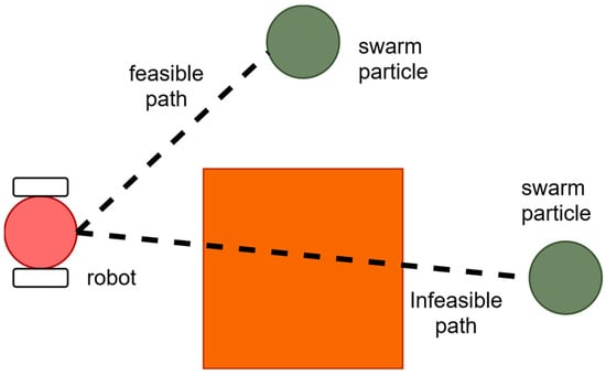
Figure 1.
An example of a path that is blocked by an obstacle.
The overall fitness function is formulated by combining the two individual fitness functions, as represented in Equation (9). In this Equation, and represent the weight factors assigned to each fitness function. These weights are fine-tuned through simulation experiments using a trial-and-error approach to achieve the desired outcome. A higher value signifies a greater emphasis on the shortest path, while a higher place more importance on collision avoidance. The goal is to optimise the path by minimising the total fitness value, as indicated by the combined fitness function, thus ensuring a balance between the two fitness functions for the best possible result.
3.4. Proposed Path Planning Scheme
In the majority of path planning problems that utilise PSO algorithm, the process typically begins with the initialisation of the particle swarm around the robot’s starting location. During each iteration, the particles’ velocity and position are updated. The algorithm determines a waypoint for the robot based on the global best position found by the particle swarm in each iteration. This iterative process continues until all particles converge on the robot’s target position. For example, if a robot’s trajectory requires ten waypoints from its starting point to its destination, the PSO algorithm is run through ten iterations in a single execution. The process is then concluded after completing these ten iterations. In this paper, unlike the traditional methods, which determine one waypoint per iteration of the PSO algorithm, we propose a different approach to determining the waypoints. Instead of calculating all waypoints in a single execution, our scheme involves running the PSO algorithm for multiple executions—one execution is run for one waypoint. For instance, if a robot’s path consists of five waypoints, the PSO algorithm will be executed for five executions, each time determining one waypoint. Additionally, the proposed path planning scheme departs from the conventional approach by initialising the particle swarm not at the robot’s starting location but within a predefined search space. This adjustment aims to improve the algorithm’s efficiency and effectiveness.
An example of waypoint generation using both basic PSO and EPSO for the initial waypoint of a robot is illustrated in Figure 2. This figure shows particles in various colours representing their positions across different iterations. In the basic PSO algorithm, a new waypoint is produced in each iteration. In contrast, the EPSO approach generates a single waypoint by completing a full execution of the PSO algorithm, rather than producing waypoints iteratively.
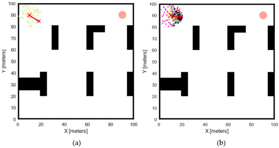
Figure 2.
Comparison of particles and waypoints generation between basic PSO and EPSO. (a) Waypoints (marked with red ‘x’) generated after one iteration using basic PSO, highlighting the incremental path refinement process; (b) waypoints (marked with red ‘x’) generated after a single execution with EPSO, demonstrating a more optimal path planning approach.
Figure 2 illustrates the operational principles of both the basic PSO algorithm and the EPSO algorithm in generating waypoints. With EPSO, we ensure that each waypoint generated by the algorithm is optimal or near-optimal. Figure 3 presents a comprehensive depiction of the paths generated by each algorithm. The comparison clearly shows that the path produced by the EPSO algorithm significantly outperforms the path generated by the basic PSO algorithm. The path derived from EPSO is notably smoother and exhibits fewer abrupt changes in direction, highlighting the superior performance and efficiency of the EPSO algorithm in path planning.
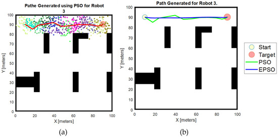
Figure 3.
Full path generated with basic PSO and EPSO algorithms. (a) Path generated with basic PSO, shown by the red line; (b) path generated with PSO and EPSO algorithm, where the green line represents the path from the basic PSO algorithm, and the blue line illustrates the more optimised path produced by the EPSO algorithm.
3.5. Dynamic Obstacle Avoidance
The proposed algorithm in this paper introduces a significant advancement over traditional PSO path planning methodologies. In conventional approaches, path planning is conducted incrementally as the robot progresses towards its goal, determining each path segment step by step. In contrast, the proposed algorithm employs a combination of global and local path planning strategies. The complete paths for all robots are computed in advance using the proposed EPSO algorithm as a global path planner before their navigation within a pre-existing simulated environment. This allows the algorithm to establish a comprehensive route for each robot before it begins its journey. By precomputing the full trajectory, the algorithm ensures that the robots follow optimised paths from their starting positions to their destinations, taking into account the overall layout of the environment. During the actual navigation phase, the algorithm integrates a sensor-based obstacle avoidance mechanism to manage dynamic obstacles effectively. This local path planning component, known as the obstacle avoidance algorithm, is crucial for maintaining safe navigation. The algorithm relies on real-time sensor data to detect and avoid collisions with dynamic obstacles within the robot’s sensing range. For this purpose, we assumed that each robot is equipped with multiple sensors, such as ultrasonic sensors, which provide comprehensive environmental data. Assuming the implementation of three HC-SR04 ultrasonic sensors, each capable of sensing distances from 2 cm to 400 cm, the robot is equipped to detect obstacles and measure distances across a broad range. However, to ensure higher accuracy and consistency in readings, we focus on a practical detection range. Thus, we assume that the sensors will be most effective within a distance of up to 250 cm. By limiting the effective detection range to 250 cm, we can reduce potential inaccuracies caused by environmental factors, signal attenuation, or reflections that might occur at the outer limits of the sensor’s capacity. This refined approach ensures that the robot relies on the most precise data for decision-making and navigation, optimising the performance of the ultrasonic sensors in real-world scenarios. As depicted, each robot is outfitted with three sensors, collectively offering a 180-degree field of view, with each individual sensor covering a 60-degree segment of the robot’s surroundings with a 250 cm distance, as illustrated in Figure 4 below.
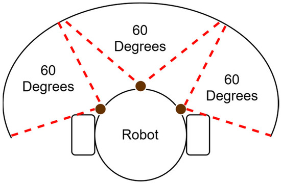
Figure 4.
Sensor angle coverage of differential drive robot with three sensors.
When a sensor detects a dynamic obstacle, it is assigned a logic value of 1, indicating the presence of the obstacle. This detection triggers an immediate response from the robot, prompting it to adjust its path to avoid the obstacle and to steer away from the direction of the obstructed sensor. This dynamic adjustment helps in navigating around obstacles in real time, ensuring that the robot does not collide with detected obstacles. In addition to avoiding static obstacles, robots are programmed to treat each other as dynamic obstacles. This feature allows robots to detect and avoid collisions with fellow robots, enhancing multi-robot operations’ overall safety and efficiency. In the case where the sensors detect no obstacles, the robot continues to move towards the waypoint that offers the shortest distance from its current position. This strategy ensures that the robot remains on an optimised path while avoiding unnecessary detours or delays. Integrating these advanced features into the proposed algorithm results in a more robust and adaptive path planning system, capable of effectively managing static and dynamic obstacles in complex environments.
Our proposed system, which equips the robot with three sensors, provides three potential solutions when the robot encounters obstacles. Each sensor offers one possible direction for the robot to move based on its detection capabilities. When two out of the three sensors detect obstacles, the robot is left with only one viable option: to move in the direction of the sensor that does not detect any obstacles. This setup ensures that the robot can avoid obstacles and continue navigating its environment under most circumstances. However, a significant limitation arises when all three sensors detect obstacles simultaneously, leaving the robot without a clear path to follow. In such a case, the robot can become stuck, unable to move in any direction. This issue becomes particularly problematic in more complex environments, where obstacles are densely packed, or when the number of robots operating within the same environment increases. In scenarios with closely arranged obstacles or multiple robots interacting, the likelihood of all sensors detecting obstacles at once becomes higher, causing the robot to be immobilised.
To address this issue and enhance the system’s performance in a highly complex environment, we propose two potential solutions to solve this problem. The first solution involves increasing the number of sensors on the robot while simultaneously decreasing the sensing range of each individual sensor. Currently, our system uses three sensors, each covering a 60-degree field of view, which limits the number of possible paths when obstacles are detected. By increasing the number of sensors and reducing the coverage angle for each sensor, the robot can detect obstacles with greater precision. This approach would provide more possible solutions and give the robot more flexibility in determining the best path to take. For example, instead of using three sensors with 60-degree coverage, we could use six sensors with 30-degree coverage each, as illustrated in Figure 5. This increased number of sensors would enable the robot to have more nuanced detection capabilities, allowing for more fine-tuned navigation decisions and reducing the likelihood of becoming stuck.
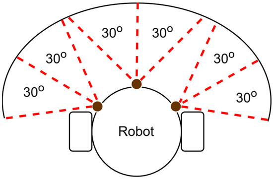
Figure 5.
Sensor angle coverage of differential drive robot with six sensors.
However, while this solution offers the robot greater precision in obstacle detection, it still fails to prevent the robot from becoming stuck when all front-facing sensors detect obstacles. In such cases, the second solution becomes a more viable option. The second solution involves providing the robot with 360-degree obstacle detection by extending sensor coverage in all directions, rather than just in front of the robot as shown in Figure 4 and Figure 5. This can be achieved by adding additional sensors around the robot’s perimeter or by using more advanced sensing technologies, such as LiDAR. A full 360-degree sensing range would allow the robot to detect obstacles from all sides, giving it more options when navigating complex environments. If the robot detects an obstacle in front, it could choose to rotate or move backward, rather than being confined to moving in the direction its front-facing sensors suggest. Figure 6 illustrates this concept, showing how sensors positioned around the entire robot would enable it to manoeuvre in any direction, avoiding situations where it would otherwise become stuck.
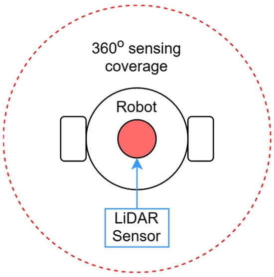
Figure 6.
Sensor angle coverage of differential drive robot with LiDAR sensor.
While the implementation of either of these solutions would significantly improve the robot’s ability to navigate more complex environments, for the purposes of simplicity in our simulation, we have chosen to use only three sensors. This basic configuration allows us to explore the fundamental capabilities of the system while providing a clear understanding of how the robot responds to obstacles in its immediate path. However, in real-world applications or more advanced simulations, both solutions, using more sensors with reduced coverage or implementing full 360-degree coverage, can be adopted to optimise the robot’s performance. Increasing the number of sensors or expanding the coverage range would enable the robot to handle more challenging navigation scenarios, minimising the risk of becoming stuck and enhancing its overall efficiency. These improvements would make the robot more adaptable to real-world applications, particularly in environments with tightly packed obstacles or where multiple robots need to operate simultaneously without collisions. Moreover, enhancing the robot’s sensing capabilities would lead to more efficient movement, reducing the time spent avoiding obstacles and lowering energy consumption.
3.6. Trajectory Smoothness with Bezier Curve
As written in the assumption, differential drive robots are characterised by their two independently driven wheels positioned on either side of the robot’s chassis, which offer a unique and versatile configuration that is assumed to be used in this context. This setup provides a high degree of manoeuvrability, allowing the robot to perform a variety of movements, including travelling in a straight line, making sharp turns, and executing smooth rotations in place. The independence of the wheels enables the robot to pivot on the spot by rotating the wheels in opposite directions and to turn by varying the relative speed of each wheel. This capability is particularly advantageous in environments where precise navigation is required.
However, the need for the robot to stop to change direction introduces a potential challenge. This discontinuity in the robot’s movement can lead to issues such as slippage or veering off the desired path. When the robot stops, the abrupt halt and subsequent change in wheel motion can cause the wheels to lose traction, especially on slippery or uneven surfaces. This can result in the robot drifting slightly from its intended course, making precise navigation more difficult. Moreover, the frequent stopping and starting required for directional changes increases energy consumption and increases wear and tear on the drive system, potentially reducing the lifespan of the robot’s mechanical components. Therefore, while the differential drive configuration offers significant advantages in terms of manoeuvrability and control, careful consideration of these factors is also necessary to ensure reliable and accurate navigation.
In this paper, we propose an approach to integrate our proposed PSO path planning algorithm with the Bezier curve trajectory smoothing algorithm to generate a smooth and continuous path for robotic navigation, thereby eliminating the need for the robots to make frequent stops and starts during their journey. While the PSO algorithm is a robust optimisation algorithm that excels in determining collision-free, optimal, and feasible paths for robots, the path generated by PSO can sometimes be jagged or contain sharp turns, which are not ideal for smooth and efficient robotic navigation. To address this problem, the Bezier curve trajectory smoothing algorithm is used to smooth out any sharp turns or abrupt changes in direction, resulting in a continuous and much smoother trajectory. Figure 7 presents an illustration of how a cubic Bezier curve is used to generate a trajectory using a start point, S (xs,ys), a destination point, D (xd,yd), and two control points, C1(xc1,yc1) and C2(xc2,yc2).
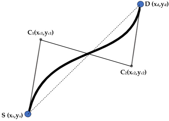
Figure 7.
Cubic Bezier curve trajectory smoothing visualisation.
A cubic Bezier curve has a third-degree polynomial with four control points (S, D, C1, C2). These control points dictate the curve’s shape, ensuring a smooth and continuous path from the starting point to the destination point. The control points C1 and C2 are critical in shaping the curve. Simply put, the control points C1 and C2 act like magnets, pulling the path towards them and creating the characteristic smooth, slowing trajectory of Bezier curves. Mathematically, the smooth Bezier curve is generated by considering the control points and using Bernstein polynomials. According to [40], the cubic Bezier curve can be expressed in Equation (10), and the Bernstein polynomials equation can be expressed in Equation (11), where represents the cubic Bezier curve with a Bernstein polynomial, represents the ith control point used in generating the curve, and represents the binomial coefficient value of the Bernstein polynomial, which can be expressed in Equation (12).
A more accurate representation of the Bezier curve can be generated by decreasing each successive increment of t from 0 to 1. For instance, if t is incremented in steps of 0.001, the Bezier curve will consist of 100 points, providing high precision. The step size of t plays a crucial role in determining how many control points along the Bezier curve are evaluated. In this case, t is incremented by 0.001 at each step. Since t ranges from 0 to 1, this small increment results in 1/0.001 = 1000 possible values for t. The curve is essentially formed by calculating the positions of points for each of these values of t. A smaller step size leads to a more precise curve because the finer the increment, the more detailed and smoother the resulting curve becomes. By sampling at more control points, gaps between them are minimised, creating a more accurate and continuous trajectory. The choice of 0.001 as the step size is deliberate, ensuring that the Bezier curve is finely sampled, producing a high-resolution and precise path that adheres closely to the control points. This level of precision is critical in applications such as robotics, where smooth, continuous paths are essential for performance and efficiency. To illustrate, if t were incremented by 0.1 instead of 0.001, the curve would consist of only 10 points, significantly reducing its smoothness. The larger gaps between points would result in a jagged trajectory, failing to capture the subtle changes in the curve’s shape. A step size of 0.1 would be inadequate for scenarios that demand smooth transitions, like robot path planning, where finer precision is necessary to achieve efficient and reliable movement. Thus, choosing a small step size like 0.001 ensures a smooth, highly accurate curve essential for applications that require precise and fluid motion.
The Bernstein polynomial, tailored explicitly for the cubic Bezier curve, is computed using Equation (11), and once the polynomial is calculated, the cubic Bezier curve can be decomposed into its x and y components, which are described by Equations (13) and (14), respectively, where and are the (x,y) coordinates of the starting point (S), destination point (D), and two control points (C1, C2)
In this paper, the waypoints of the robot’s pathway established by our proposed PSO algorithm are extracted to serve as the foundational points for the Bezier curve smooth trajectory. Initially, the Bernstein basis function is calculated for each robot, forming the Bezier curve’s mathematical foundation. Next, the coordinates of the Bezier curve control points are computed by summing the element-wise product of the robot’s waypoints and the Bernstein basis function, ensuring that the influence of each waypoint is appropriately factored into the final smooth path. Finally, the Bezier curve points are plotted for each robot, illustrating the smooth trajectory from the starting point to the destination point. During the simulation, the robot will travel from its initial position to the destination, following the smooth path generated by the Bezier curve algorithm.
3.7. Flowchart of EPSO Path Planning Algorithm
In this paper, we refer to the combination of our proposed PSO path planning algorithm and the Bezier curve trajectory smoothing algorithm as EPSO. The flowchart of the EPSO algorithm is illustrated in Figure 8.
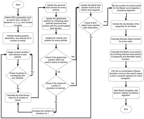
Figure 8.
Flowchart of EPSO algorithm.
4. Results
This section presents the simulation results obtained from the basic PSO path planning algorithm and our proposed EPSO algorithm. We begin by introducing the relevant details of the simulation setup. Next, we describe the parameter settings used to configure the PSO algorithms and the Bezier curve trajectory smoothing algorithm. Following this, we conduct a comparative simulation and discussion using the basic PSO algorithm and our proposed EPSO algorithm to evaluate their performance in terms of path length, execution time, and number of turn points.
4.1. Simulation Setup
The simulations were conducted using MATLAB R2022b on a Windows 11 computer equipped with an Intel Core i5 processor running at 2.5 GHz and 24 GB of RAM. The simulations take place in a 2D simulated workspace measuring 100 m by 100 m. The environment includes static obstacles of various shapes and sizes to mimic realistic scenarios. Additionally, each robot is considered a dynamic obstacle to the others, adding a layer of complexity as they must avoid collisions while following their paths. To assess the algorithms, two distinct simulation scenarios were designed as shown in Figure 9. The robots used in the simulations are assumed to be differential drive robots, which are common in practical applications due to their simple control and manoeuvrability. All robots in the simulation are identical, ensuring consistency in the evaluation process. Their maximum speed is set to a fixed velocity of 2 m per second throughout the whole simulation. Unlike standard simulations with fixed time steps, the current setup uses an implicit time step determined by the duration of each loop iteration. This duration fluctuates based on task complexity, including distance calculations, heading adjustments, and position updates. As a result, the simulation dynamically adjusts to the computational load, enabling real-time updates of robot movements and environmental interactions. For instance, if a robot begins at position (0, 0) and moves at 2 m per second, its position updates depend on the loop iteration time. If each loop takes about 0.1 s, the robot will be at (2, 0) after 1 s of simulated time. This approach enhances collision avoidance by allowing continuous recalculation of positions and timely detection of potential collisions, reducing the impact of longer iteration times.
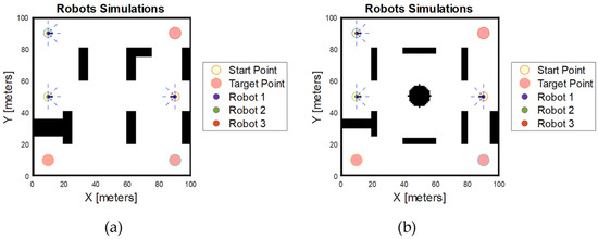
Figure 9.
Robot 2D simulation workspace. (a) First scenario; (b) second scenario.
4.2. Parameters of EPSO Used in the Simulations
The configuration of the EPSO algorithm involves setting parameters for both the PSO algorithm and the Bezier curve trajectory smoothing algorithm. The parameter settings for both the PSO algorithm and Bezier curve algorithm employed in this simulation are as follows:
- (1)
- Swarm size: 50 particles;
- (2)
- Maximum iteration (itertotal): 30 iterations;
- (3)
- Maximum inertia weight (): 0.95;
- (4)
- Minimum inertia weight (): 0.4;
- (5)
- Maximum cognitive parameter () and maximum social parameter (): 2.0;
- (6)
- Minimum cognitive parameter () and minimum social parameter (): 0.5;
- (7)
- Number of control points used in Bezier curve calculation: 100.
Each robot in the simulation is assigned a unique starting position and a distinct destination point. These positions are strategically chosen to ensure that the robots navigate through the 2D workspace while avoiding obstacles and potential collisions with each other. The unique starting positions and destination points are designed to simulate real-world scenarios where multiple robots operate simultaneously in a shared environment. The starting positions are scattered throughout the workspace, ensuring that the robots do not start too close to each other, which would make the simulation less challenging. Similarly, the destination points are distributed so that the robots must traverse significant portions of the workspace to reach their goals. The starting coordinate and destination point for each robot are set as stated in Table 1.

Table 1.
Starting position and destination point for each robot.
4.3. Comparison between EPSO and Basic PSO
By using the parameters’ values, the performance of EPSO, which consists of our proposed PSO algorithm with the new path planning scheme, obstacle avoidance algorithm, and Bezier curve trajectory smoothing algorithm, is compared with the performance with the basic PSO algorithm in two different scenarios.
4.3.1. First Scenario
Figure 10 shows the particles generated for each iteration and the path generated for each robot using the basic PSO algorithm in the first scenario. The particles, each represented by a different colour, indicate the positions of individual particles within the swarm. In every iteration, after the evaluation of the fitness value of all particles, the particle with the lowest fitness value is chosen as the optimal waypoint for the robot. After all the waypoints are calculated, the path of the robot is generated by connecting these waypoints together. The total waypoints generated for each robot are 18, 13, and 13 for robots 1, 2, and 3, respectively.
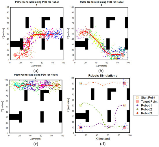
Figure 10.
Simulation results obtained using basic PSO algorithm in the first scenario. (a) Particle positions generated in each iteration for Robot 1; (b) particle positions generated for each iteration for Robot 2; (c) particle positions generated in each iteration for Robot 3; (d) robot simulation result.
Figure 11 illustrates the simulation results obtained using the proposed EPSO algorithm in the first scenario. The simulation results show that the waypoints generated for each robot are 12, 12, and 10 for robots 1, 2, and 3, respectively. The robot trajectories coloured in green represent the path generated with the basic PSO algorithm, while the trajectories coloured in blue represent the smooth trajectory generated using our proposed MPSO algorithm with the new path planning scheme and the Bezier curve trajectory smoothing algorithm.

Figure 11.
Simulation results obtained using EPSO and PSO algorithms in the first scenario. (a) Path generated for Robot 1; (b) path generated for Robot 2; (c) path generated for Robot 3; (d) robot simulation result.
Simulations were conducted five times for each algorithm to capture the average performance and the standard deviation of the results. The outcomes of these simulations for both the basic PSO and EPSO algorithms are shown in Table 2. One of the key factors analysed in the simulation was the number of turn points for the robots. These turn points represent instances where the robots’ paths deviate by more than a specified threshold as they travel from one waypoint to the next. In this study, any directional change exceeding a predefined threshold of 5 degrees is considered a turn point, potentially requiring the robot to stop and reorient before proceeding. Conversely, changes below this threshold allow the robot to maintain its momentum and follow a smoother trajectory. This threshold angle is critical because frequent directional changes can negatively impact the robot’s smoothness of travel, energy consumption, and overall path efficiency. Fewer turn points imply that the path is smoother, reducing the need for frequent stops and increasing energy efficiency. By assessing the number of turn points generated by each algorithm, we can evaluate the ability of the path planning algorithms to provide optimised routes that minimise abrupt stops and directional changes.
Table 2.
Simulation results generated for both basic PSO and EPSO in the first scenario.
In the first scenario simulated, the basic PSO algorithm struggled to produce smooth trajectories, leading to a higher number of turn points compared to the EPSO algorithm. As a result, robots following paths generated by basic PSO needed to stop more frequently and use more energy. In contrast, the EPSO algorithm, despite a marginally longer execution time, generated smoother and shorter paths by leveraging a new path planning scheme and incorporating the Bezier curve smoothing algorithm. This enabled the EPSO to reduce the number of sharp turns, leading to more efficient robot navigation and lower energy consumption.
The data from five simulation runs reveal significant differences in performance between the two algorithms. Over multiple runs, the basic PSO algorithm showed higher variability, with a greater standard deviation in both path length and execution time. This inconsistency suggests that basic PSO’s performance is less reliable, which could be problematic in real-world applications where predictable outcomes are crucial. EPSO, on the other hand, consistently outperformed the basic PSO in generating more efficient paths. Based on the result, EPSO was able to reduce the path length by as much as 24.67%, which has significant implications for applications where minimising travel distance and energy use are important. The EPSO algorithm also reduced the number of disruptive turns by 200%, leading to smoother navigation and fewer stops for reorientation. This makes EPSO far more effective in terms of optimising path efficiency.
Interestingly, the results also reveal that Robot 1 follows different paths with each algorithm. Robot 1 took a longer path using the basic PSO, whereas EPSO ensured that the path was optimal or near-optimal. This observation underscores EPSO’s ability to generate more efficient routes compared to basic PSO.
However, these improvements come at a slight cost. The EPSO algorithm required up to 21.76% more execution time compared to basic PSO. This additional time is due to the more complex calculations involved in calculating the robot’s waypoints using MPSO and the additional step in generating smoother paths using the Bezier curve trajectory smoothing algorithm. Although this longer planning time may not be a major issue in scenarios where time is less critical, it could be a limitation in real-time or time-sensitive applications where rapid decision-making is required. Despite this trade-off, EPSO’s ability to produce smoother, more efficient paths with fewer directional changes represents a significant advantage over basic PSO.
4.3.2. Second Scenario
Figure 12 shows the particles generated for each iteration and the path generated for each robot using the basic PSO algorithm in the second scenario. The total waypoints generated for each robot are 12, 12, and 11 for robots 1, 2, and 3, respectively.
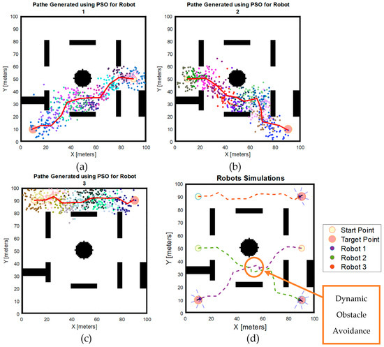
Figure 12.
Simulation results obtained using basic PSO algorithm in the second scenario. (a) Particle positions generated in each iteration for Robot 1; (b) particle positions generated for each iteration for Robot 2; (c) particle positions generated in each iteration for Robot 3; (d) robot simulation result.
A more detailed visualisation of the dynamic collision avoidance simulation that occurred in Figure 12 is provided in Figure 13. In Figure 13a, Robot 1 and Robot 2 detect each other, activating the collision avoidance algorithm. Figure 13b,c show that after detection, both robots adjust their directions based on their sensors’ status to prevent a collision. They navigate towards the direction indicated by sensors that do not detect obstacles while also aiming for the shortest path to the next waypoint. Given that three sensors are utilised, the robot has three potential paths to choose from, each determined by the status of the sensors and the length of the path. Subsequently, as illustrated in Figure 13d, Robot 1 halts because all three of its sensors detect obstacles, while Robot 2 moves to an obstacle-free position. Once Robot 2 has cleared the area, Robot 1 resumes movement when its sensors no longer detect obstacles, as shown in Figure 13e. Finally, Figure 13f depicts both robots returning to their original paths and continuing to navigate following the original path.
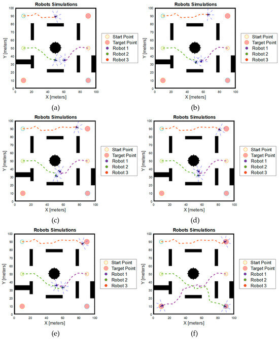
Figure 13.
Dynamic collision avoidance during the simulation. (a) Robots 1 and 2 detect each other, triggering the avoidance algorithm; (b) both robots change direction to avoid a collision; (c) Robot 1 stops as all sensors detect obstacles, while Robot 2 moves to a clear position; (d) Robot 1 remain stopped as all sensors still detecting obstacles; (e) Robot 1 resume once obstacles are cleared; (f) complete paths for all robots.
Figure 14 illustrates the simulation results obtained using the proposed EPSO algorithm in the second scenario. The simulation results show that the waypoints generated for each robot are 11, 12, and 9 for robots 1, 2, and 3, respectively. Similar to the simulation conducted with the first scenario, the robot trajectories coloured in green represent the path generated using the basic PSO algorithm, while the trajectories coloured in blue represent the smooth trajectory generated with the proposed MPSO algorithm and the Bezier curve trajectory smoothing algorithm.
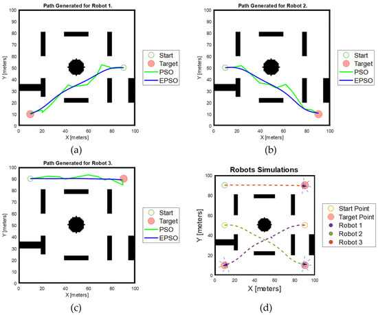
Figure 14.
Simulation results obtained using EPSO and PSO algorithms in the second scenario. (a) Path generated for Robot 1; (b) Path generated for Robot 2; (c) path generated for Robot 3; (d) robot simulation result.
Consistent with the methodology employed in Scenario 1, simulations were executed five times for each algorithm to compute the average results and standard deviations. These simulations aimed to assess the performance of the basic PSO and EPSO algorithms. The detailed outcomes of these simulations are summarised in Table 3.
Table 3.
Simulation result for both basic PSO and EPSO algorithm in Scenario 2.
The results indicate a notable distinction between the two algorithms regarding the number of required turns. Specifically, robots utilising the EPSO algorithm achieved one turn for Robot 1 and zero turns for Robot 2 and Robot 3, signifying a highly efficient path with no abrupt changes in direction. In contrast, robots operating under the basic PSO algorithm exhibited a considerable number of turns, attributed to the less smooth path generation capabilities of the basic PSO. This inefficiency in path smoothness results in increased energy consumption for robots using the basic PSO algorithm, as they must frequently adjust their trajectories. The findings from Scenario 2 mirror those observed in Scenario 1. In this scenario, the EPSO algorithm consistently enabled robots to traverse shorter paths compared to those generated by the basic PSO algorithm. This improvement in path length demonstrates the EPSO algorithm’s effectiveness in optimising route efficiency. Further analysis reveals that the basic PSO algorithm is characterised by a higher standard deviation in both path length and execution time compared to the EPSO algorithm. This indicates that the EPSO algorithm provides greater stability and consistency in performance. Specifically, the EPSO algorithm excels in producing paths that are, on average, 15.71% shorter and achieves a dramatic 200% reduction in the number of turns required for the robots to stop and reorient themselves. Similar to Scenario 1, the EPSO algorithm requires up to 17.55% more execution time than the basic PSO algorithm.
In addition to conducting an extensive comparative analysis between the basic PSO algorithm and its enhanced counterpart, the EPSO algorithm, we expanded our evaluation to encompass a variety of other well-established path planning algorithms. The primary objective of this research was to assess the relative performance of these algorithms, particularly in comparison to EPSO, which is positioned as a more advanced and optimised solution for complex path planning tasks. The algorithms included in this comprehensive assessment were Ant Colony Optimisation (ACO), Genetic Algorithm (GA), A*, and Rapidly Exploring Random Tree (RRT). Each simulation was repeated five times to obtain the average values and standard deviations for critical performance metrics, such as path length and execution time.
The results of these simulations, as presented in Figure 15 and Table 4, offer a detailed comparative overview of each algorithm’s ability to identify the shortest path in a given environment, as well as the algorithms’ computational efficiency. From our analysis, it is evident that the EPSO algorithm consistently outperforms the other algorithms in terms of key performance indicators, notably path length and the number of turns. Specifically, EPSO demonstrates an outstanding ability to determine the optimal path between the starting and goal positions. When EPSO is compared to other algorithms, several notable patterns emerge. For instance, the ACO algorithm generates a distinctly different path compared to the others, and this path is the longest among all those evaluated. Not only does ACO produce the longest path, but it also has the highest execution time, making it less favourable for real-time or time-sensitive applications. In contrast, EPSO achieved zero turns in the paths it generated, which is a testament to its ability to find smoother and more direct routes. RRT, on the other hand, resulted in the highest number of turns, indicating that while it may find feasible paths, these paths are often less efficient in terms of distance and trajectory smoothness. Despite EPSO having the second-highest execution time after ACO, it was able to consistently generate the shortest path, making it a more balanced solution in terms of both path length and computational demands. Additionally, among the algorithms tested, the A* algorithm, which is relatively simpler, was able to generate paths with the fastest execution times; however, these paths were often not the shortest, revealing a trade-off between speed and path optimisation.
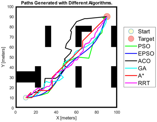
Figure 15.
Paths generated with different path planning algorithms.
Table 4.
Simulation results for different path planning algorithms.
The performance metrics further reveal a critical distinction between traditional and meta-heuristic algorithms. Traditional algorithms, such as A* and RRT, are capable of generating paths with relatively low execution times, making them attractive for applications where computational speed is a priority. However, these algorithms tend to produce longer paths compared to those generated by EPSO, which highlights their limitation in terms of path optimisation. This comprehensive evaluation clearly underscores the significant advantages of employing the EPSO algorithm for complex path planning tasks. EPSO’s ability to consistently deliver shorter path lengths, while maintaining competitive computational performance, makes it an ideal choice for applications that require optimal pathfinding solutions.
5. Discussion
The results obtained from the simulations comparing the basic PSO algorithm with the EPSO algorithm reveal substantial differences in their performance for multi-robot path planning tasks. The EPSO algorithm demonstrates a significant enhancement in generating smoother and more efficient paths, as evidenced by the minimal or zero turn points recorded for most robots when using EPSO in both Scenario 1 and Scenario 2. This contrasts sharply with the basic PSO algorithm, which consistently results in a higher number of turns. Such frequent directional changes necessitate more stops and reorientations, leading to increased energy consumption and extended travel time. This underscores the advantage of the EPSO algorithm in creating more efficient paths, owing to its incorporation of the Bezier curve trajectory smoothing method. In both scenarios, the EPSO algorithm not only generates smoother paths but also consistently produces shorter paths compared to the basic PSO algorithm. This improvement in path length and smoothness is significant. The basic PSO algorithm, in contrast, exhibits a higher standard deviation in path length and execution time, indicating less consistency and reliability in path planning.
Although the EPSO algorithm does entail slightly longer execution times due to the additional computations required for trajectory smoothing, this trade-off is well justified by the substantial improvements observed in path quality and overall travel efficiency. The smoother trajectories produced by EPSO lead to a reduction in the number of turns and a decrease in overall travel distance.
From these results, it can be concluded that the EPSO algorithm surpasses the basic PSO algorithm in terms of path smoothness, efficiency, and overall effectiveness in multi-robot path planning. The integration of Bezier curve trajectory smoothing substantially enhances the quality of the generated paths, positioning EPSO as a highly effective approach for optimising multi-robot navigation. Despite the minor increase in execution time, the benefits of reduced path length, fewer turns, and improved travel efficiency make EPSO a superior choice for complex multi-robot path planning scenarios.
6. Conclusions
In conclusion, the Enhanced Particle Swarm Optimisation (EPSO) algorithm, which integrates the new path planning scheme with the Bezier curve trajectory smoothing technique, demonstrates superior performance in multi-robot path planning compared to the basic PSO algorithm. The simulations indicate that EPSO generates smoother, shorter paths with fewer directional changes, reducing the need for frequent stops and reorientations. This results in more efficient navigation, lower energy consumption, and improved overall performance. Despite the slightly increased execution time due to the additional computations required for trajectory smoothing, the advantages of EPSO in terms of path quality and travel efficiency make it a highly effective solution for complex multi-robot navigation tasks. The findings underscore the value of trajectory smoothing in enhancing the capabilities of PSO-based path planning algorithms, offering significant improvements in robotic navigation and coordination.
Author Contributions
Conceptualisation, S.D.; methodology, Y.-L.P., Z.-Y.L. and S.D.; software, Y.-L.P.; validation, D.W.K.N.; formal analysis, Y.-L.P., Z.-Y.L. and S.D.; investigation, S.D., H.L. and D.W.K.N.; resources, C.-H.G. and H.L.; writing—original draft, Y.-L.P., Z.-Y.L. and S.D.; writing—review and editing, Y.-L.P., S.D., C.-H.G., B.-H.K., H.L. and D.W.K.N.; visualisation, Y.-L.P. and Z.-Y.L.; supervision, S.D., C.-H.G. and B.-H.K. All authors have read and agreed to the published version of the manuscript.
Funding
This research received no external funding.
Institutional Review Board Statement
Not applicable.
Informed Consent Statement
Not applicable.
Data Availability Statement
No data were used for the research described in the article.
Conflicts of Interest
The authors declare no conflicts of interest.
References
- Abujabal, N.A.; Rabie, T.; Kamel, I. Path Planning Techniques for Multi-Robot Systems: A Systematic Review. In Proceedings of the 2023 15th International Conference on Innovations in Information Technology (IIT), Al Ain, United Arab Emirates, 14–15 November 2023; IEEE: Piscataway, NJ, USA, 2023; pp. 1–6. [Google Scholar]
- Abujabal, N.; Fareh, R.; Sinan, S.; Baziyad, M.; Bettayeb, M. A Comprehensive Review of the Latest Path Planning Developments for Multi-Robot Formation Systems. Robotica 2023, 41, 2079–2104. [Google Scholar] [CrossRef]
- Atiyah, A.N.; Adzhar, N.; Jaini, N.I. An Overview: On Path Planning Optimization Criteria and Mobile Robot Navigation. J. Phys. Conf. Ser. 2021, 1988, 012036. [Google Scholar] [CrossRef]
- Madridano, Á.; Al-Kaff, A.; Martín, D.; de la Escalera, A. Trajectory Planning for Multi-Robot Systems: Methods and Applications. Expert Syst. Appl. 2021, 173, 114660. [Google Scholar] [CrossRef]
- Karur, K.; Sharma, N.; Dharmatti, C.; Siegel, J.E. A Survey of Path Planning Algorithms for Mobile Robots. Vehicles 2021, 3, 448–468. [Google Scholar] [CrossRef]
- Koubaa, A.; Bennaceur, H.; Chaari, I.; Trigui, S.; Ammar, A.; Sriti, M.-F.; Alajlan, M.; Cheikhrouhou, O.; Javed, Y. Introduction to Mobile Robot Path Planning. Robot. Path Plan. Coop. Found. Algorithms Exp. 2018, 772, 3–12. [Google Scholar]
- Lin, S.; Liu, A.; Wang, J.; Kong, X. A Review of Path-Planning Approaches for Multiple Mobile Robots. Machines 2022, 10, 773. [Google Scholar] [CrossRef]
- Chand, P.; Carnegie, D.A. A Two-Tiered Global Path Planning Strategy for Limited Memory Mobile Robots. Robot. Auton. Syst. 2012, 60, 309–321. [Google Scholar] [CrossRef]
- Das, P.K.; Behera, H.S.; Panigrahi, B.K. A Hybridisation of an Improved Particle Swarm Optimisation and Gravitational Search Algorithm for Multi-Robot Path Planning. Swarm. Evol. Comput. 2016, 28, 14–28. [Google Scholar] [CrossRef]
- Patle, B.K.; Babu, L.G.; Pandey, A.; Parhi, D.R.K.; Jagadeesh, A. A Review: On Path Planning Strategies for Navigation of Mobile Robot. Def. Technol. 2019, 15, 582–606. [Google Scholar] [CrossRef]
- Lamini, C.; Fathi, Y.; Benhlima, S. H-MAS Architecture and Reinforcement Learning Method for Autonomous Robot Path Planning. In Proceedings of the 2017 Intelligent Systems and Computer Vision (ISCV), Fez, Morocco, 17–19 April 2017; IEEE: Piscataway, NJ, USA, 2017; pp. 1–7. [Google Scholar]
- Koren, Y.; Borenstein, J. Potential Field Methods and Their Inherent Limitations for Mobile Robot Navigation. In Proceedings of the 1991 IEEE International Conference on Robotics and Automation, Sacramento, CA, USA, 9–11 April 1991; pp. 1398–1404. [Google Scholar]
- Matoui, F.; Boussaid, B.; Metoui, B.; Frej, G.B.; Abdelkrim, M.N. Path Planning of a Group of Robots with Potential Field Approach: Decentralised Architecture. IFAC-PapersOnLine 2017, 50, 11473–11478. [Google Scholar] [CrossRef]
- Wu, Z.; Su, W.; Li, J. Multi-Robot Path Planning Based on Improved Artificial Potential Field and B-Spline Curve Optimization. In Proceedings of the 2019 Chinese Control Conference (CCC), Guangzhou, China, 27–30 July 2019; IEEE: Piscataway, NJ, USA, 2019; pp. 4691–4696. [Google Scholar]
- Khatib, O. Real-Time Obstacle Avoidance for Manipulators and Mobile Robots. Int. J. Robot. Res. 1986, 5, 90–98. [Google Scholar] [CrossRef]
- Ma, X.; Gong, R.; Tan, Y.; Mei, H.; Li, C. Path Planning of Mobile Robot Based on Improved PRM Based on Cubic Spline. Wirel. Commun. Mob. Comput. 2022, 2022, 1632698. [Google Scholar] [CrossRef]
- Replogle, B.; Yu, X.-H. A Fuzzy Inference System on Probabilistic Roadmap for Multi-Robot Path Planning. In Proceedings of the 2023 WRC Symposium on Advanced Robotics and Automation (WRC SARA), Beijing, China, 19 August 2023; IEEE: Piscataway, NJ, USA, 2023; pp. 504–509. [Google Scholar]
- Li, Y.; Cui, R.; Yang, C.; Xu, D. Multi-Robot Path Planning Based on the Developed RRT* Algorithm. In Proceedings of the 32nd Chinese Control Conference, Xi’an, China, 26 July 2013; pp. 7049–7053. [Google Scholar]
- Connell, D.; Manh La, H. Extended Rapidly Exploring Random Tree–Based Dynamic Path Planning and Replanning for Mobile Robots. Int. J. Adv. Robot. Syst. 2018, 15, 172988141877387. [Google Scholar] [CrossRef]
- Kiadi, M.; García, E.; Villar, J.R.; Tan, Q. A*-Based Co-Evolutionary Approach for Multi-Robot Path Planning with Collision Avoidance. Cybern. Syst. 2023, 54, 339–354. [Google Scholar] [CrossRef]
- Wang, W.; Goh, W.-B. Multi-Robot Path Planning with the Spatio-Temporal A* Algorithm and Its Variants. In Advanced Agent Technology: AAMAS 2011 Workshops, AMPLE, AOSE, ARMS, DOCM 3 AS, ITMAS, Taipei, Taiwan, 2–6 May 2011. Revised Selected Papers 10; Springer: Berlin/Heidelberg, Germany, 2012; pp. 313–329. [Google Scholar]
- Chen, X.; Zhang, X.; Huang, W.; Liu, S.; Dai, H. Coordinated Optimal Path Planning of Multiple Substation Inspection Robots Based on Conflict Detection. In Proceedings of the 2019 Chinese Automation Congress (CAC), Hangzhou, China, 22–24 November 2019; IEEE: Piscataway, NJ, USA, 2019; pp. 5069–5074. [Google Scholar]
- Bae, H.; Kim, G.; Kim, J.; Qian, D.; Lee, S. Multi-Robot Path Planning Method Using Reinforcement Learning. Appl. Sci. 2019, 9, 3057. [Google Scholar] [CrossRef]
- Wang, Z.; Shi, Z.; Li, Y.; Tu, J. The Optimization of Path Planning for Multi-Robot System Using Boltzmann Policy Based Q-Learning Algorithm. In Proceedings of the 2013 IEEE International Conference on Robotics and Biomimetics (ROBIO), Shenzhen, China, 12–14 December 2013; IEEE: Piscataway, NJ, USA, 2013; pp. 1199–1204. [Google Scholar]
- TAN, G.-Z. Ant Colony System Algorithm for Real-Time Globally Optimal Path Planning of Mobile Robots. ACTA Autom. Sin. 2007, 33, 0279. [Google Scholar] [CrossRef]
- Yanes Luis, S.; Peralta, F.; Tapia Córdoba, A.; Rodríguez del Nozal, Á.; Toral Marín, S.; Gutiérrez Reina, D. An Evolutionary Multi-Objective Path Planning of a Fleet of ASVs for Patrolling Water Resources. Eng. Appl. Artif. Intell. 2022, 112, 104852. [Google Scholar] [CrossRef]
- Biswas, S.; Anavatti, S.G.; Garratt, M.A. Obstacle Avoidance for Multi-Agent Path Planning Based on Vectorised Particle Swarm Optimisation. In Intelligent and Evolutionary Systems, Proceedings of the 20th Asia Pacific Symposium, IES 2016, Canberra, Australia, November 2016, Proceedings; Springer: Berlin/Heidelberg, Germany, 2017; pp. 61–74. [Google Scholar]
- Ayari, A.; Bouamama, S. A New Multi-Robot Path Planning Algorithm: Dynamic Distributed Particle Swarm Optimization. Robot. Biomim. 2017, 4, 1–15. [Google Scholar] [CrossRef]
- Das, P.K.; Sahoo, B.M.; Behera, H.S.; Vashisht, S. An Improved Particle Swarm Optimisation for Multi-Robot Path Planning. In Proceedings of the 2016 International Conference on Innovation and Challenges in Cyber Security (ICICCS-INBUSH), Greater Noida, India, 3–5 February 2016; IEEE: Piscataway, NJ, USA, 2016; pp. 97–106. [Google Scholar]
- Das, P.K.; Behera, H.S.; Das, S.; Tripathy, H.K.; Panigrahi, B.K.; Pradhan, S.K. A Hybrid Improved PSO-DV Algorithm for Multi-Robot Path Planning in a Clutter Environment. Neurocomputing 2016, 207, 735–753. [Google Scholar] [CrossRef]
- Das, P.K.; Jena, P.K. Multi-Robot Path Planning Using Improved Particle Swarm Optimisation Algorithm through Novel Evolutionary Operators. Appl. Soft. Comput. 2020, 92, 106312. [Google Scholar] [CrossRef]
- Li, X.; Wu, D.; He, J.; Bashir, M.; Liping, M. An Improved Method of Particle Swarm Optimisation for Path Planning of Mobile Robot. J. Control. Sci. Eng. 2020, 2020, 3857894. [Google Scholar] [CrossRef]
- Eberhart, R.; Kennedy, J. A New Optimizer Using Particle Swarm Theory. In Proceedings of the MHS’95. Proceedings of the Sixth International Symposium on Micro Machine and Human Science, Nagoya, Japan, 4–6 October 1995; IEEE: Piscataway, NJ, USA, 1995; pp. 39–43. [Google Scholar]
- Shami, T.M.; El-Saleh, A.A.; Alswaitti, M.; Al-Tashi, Q.; Summakieh, M.A.; Mirjalili, S. Particle Swarm Optimisation: A Comprehensive Survey. IEEE Access 2022, 10, 10031–10061. [Google Scholar] [CrossRef]
- Doctor, S.; Venayagamoorthy, G.K.; Gudise, V.G. Optimal PSO for Collective Robotic Search Applications. In Proceedings of the 2004 Congress on Evolutionary Computation (IEEE Cat. No.04TH8753), Portland, OR, USA, 19–23 June 2004; IEEE: Piscataway, NJ, USA, 2004; pp. 1390–1395. [Google Scholar]
- Zhang, Y.; Gong, D.; Zhang, J. Robot Path Planning in Uncertain Environment Using Multi-Objective Particle Swarm Optimisation. Neurocomputing 2013, 103, 172–185. [Google Scholar] [CrossRef]
- Grandi, R.; Falconi, R.; Melchiorri, C. A Navigation Strategy for Multi-Robot Systems Based on Particle Swarm Optimisation Techniques. IFAC Proc. Vol. 2012, 45, 331–336. [Google Scholar] [CrossRef]
- Chołodowicz, E.; Figurowski, D. Mobile Robot Path Planning with Obstacle Avoidance Using Particle Swarm Optimisation. Pomiary Autom. Robot. 2017, 21, 59–68. [Google Scholar] [CrossRef]
- Song, B.; Wang, Z.; Zou, L. An Improved PSO Algorithm for Smooth Path Planning of Mobile Robots Using Continuous High-Degree Bezier Curve. Appl. Soft. Comput. 2021, 100, 106960. [Google Scholar] [CrossRef]
- Soto, D.; Soto, W. Path Planning for Mobile Robot Based on Cubic Bézier Curve and Adaptive Particle Swarm Optimization (A2PSO). In Advances in Emerging Trends and Technologies; Springer: Berlin/Heidelberg, Germany, 2020; pp. 432–441. [Google Scholar]
- Poy, Y.L.; Darmaraju, S.; Kwan, B.-H. Multi-Robot Path Planning Using Modified Particle Swarm Optimisation. In Proceedings of the 2023 IEEE International Conference on Automatic Control and Intelligent Systems (I2CACIS), Shah Alam, Malaysia, 17 June 2023; IEEE: Piscataway, NJ, USA, 2023; pp. 225–230. [Google Scholar]
- Shi, Y.; Eberhart, R. A Modified Particle Swarm Optimizer. In Proceedings of the 1998 IEEE International Conference on Evolutionary Computation Proceedings. IEEE World Congress on Computational Intelligence (Cat. No.98TH8360), Anchorage, AK, USA, 4–9 May 1998; IEEE: Piscataway, NJ, USA; pp. 69–73. [Google Scholar]
- Ravankar, A.; Ravankar, A.A.; Kobayashi, Y.; Hoshino, Y.; Peng, C.-C. Path Smoothing Techniques in Robot Navigation: State-of-the-Art, Current and Future Challenges. Sensors 2018, 18, 3170. [Google Scholar] [CrossRef]
- Xu, L.; Song, B.; Cao, M. A New Approach to Optimal Smooth Path Planning of Mobile Robots with Continuous-Curvature Constraint. Syst. Sci. Control. Eng. 2021, 9, 138–149. [Google Scholar] [CrossRef]
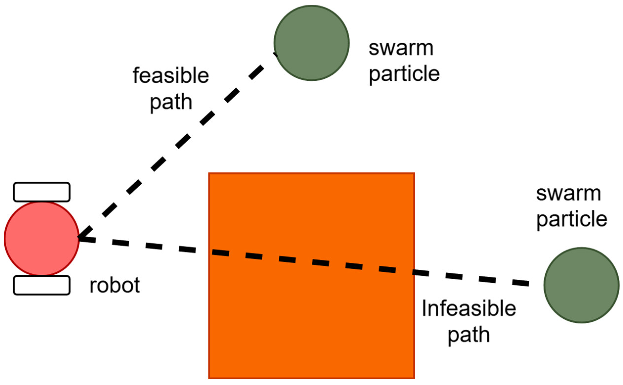
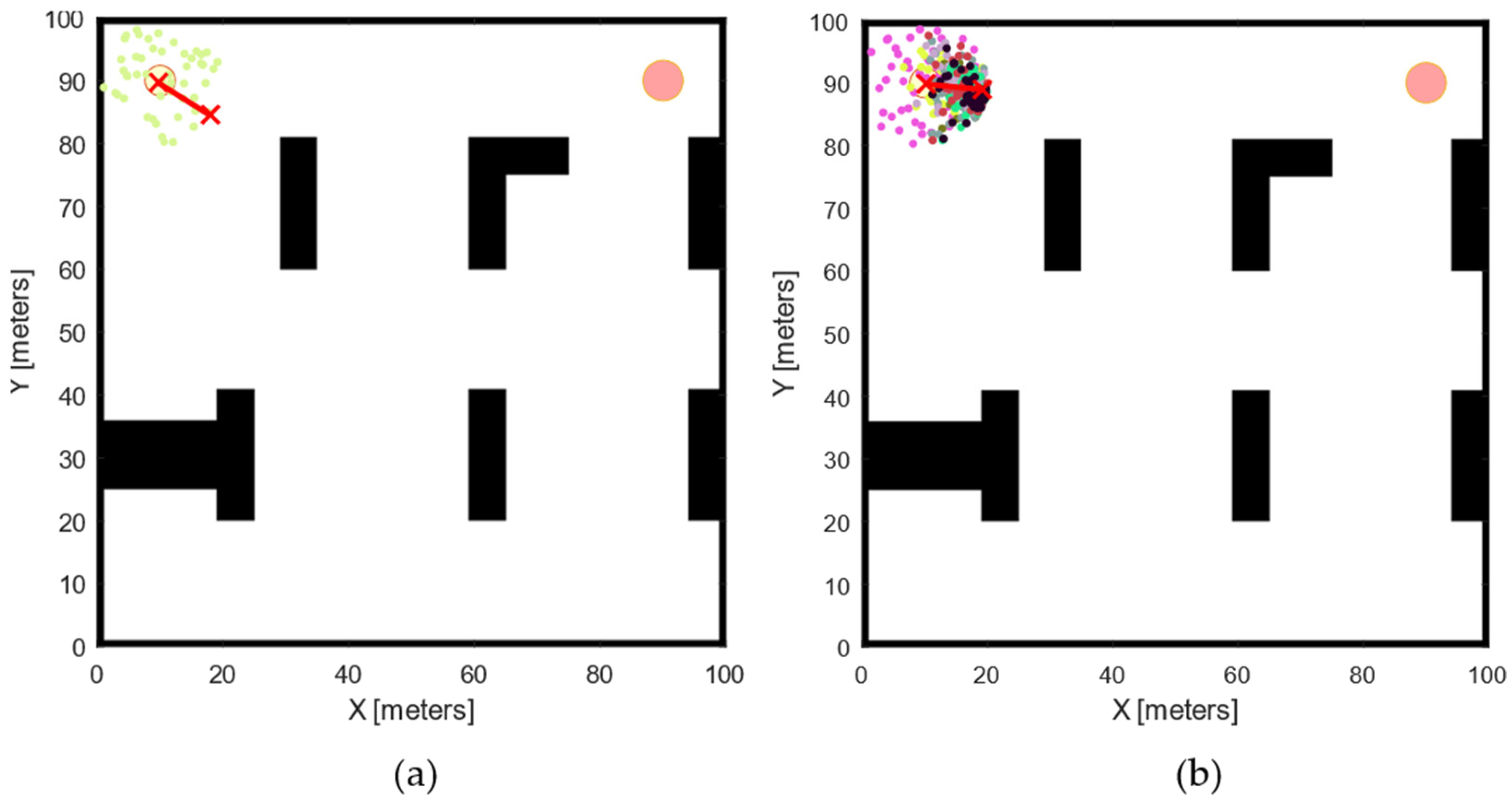
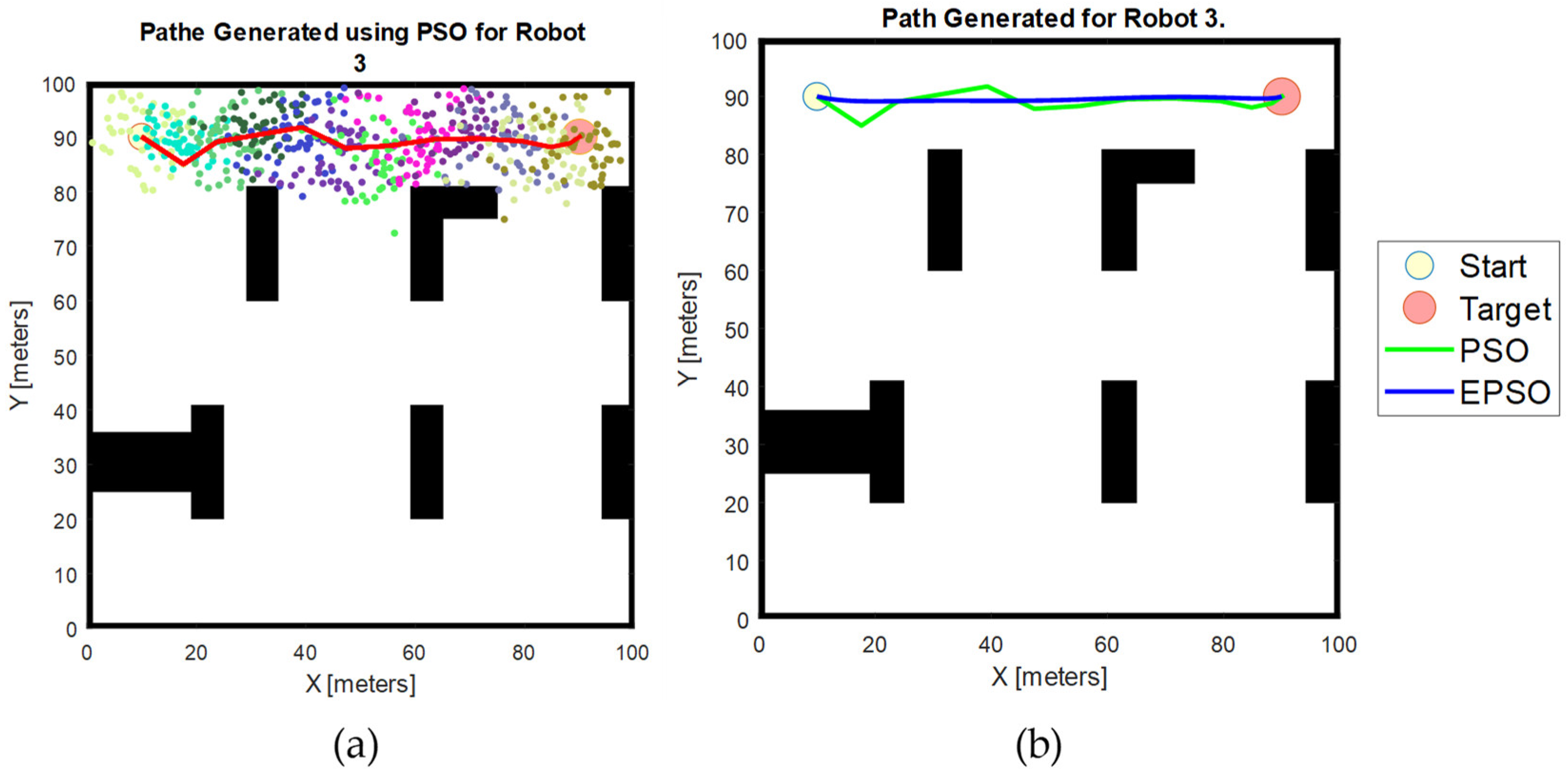
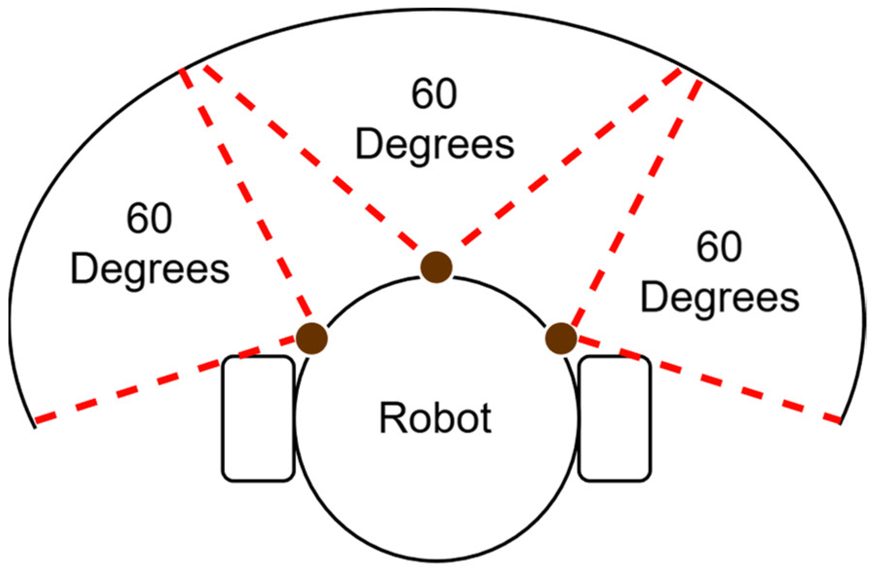
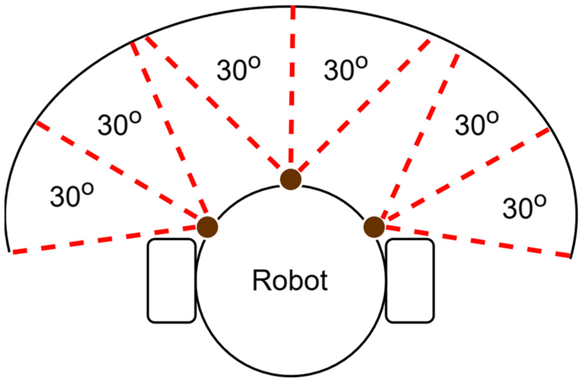
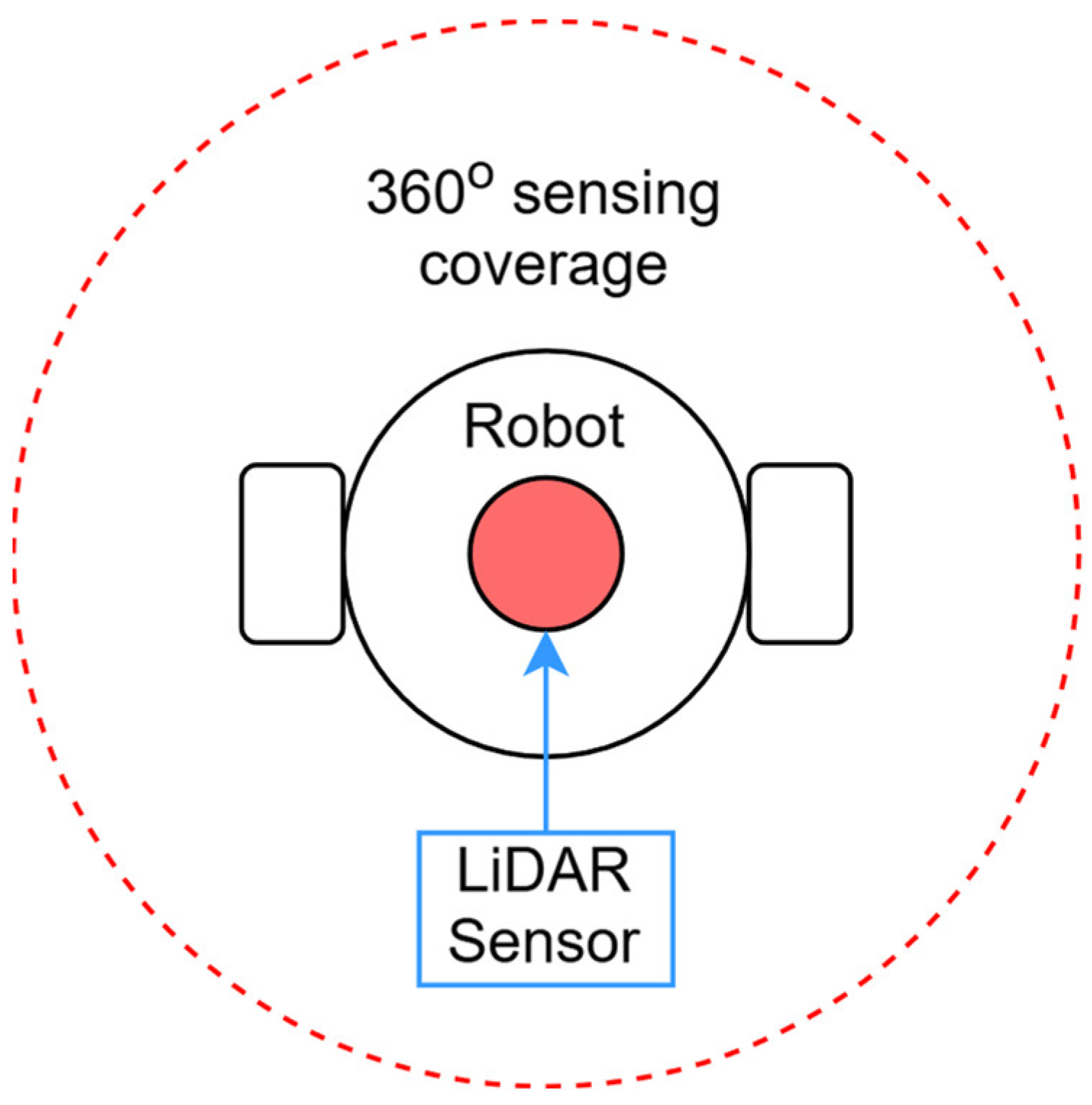
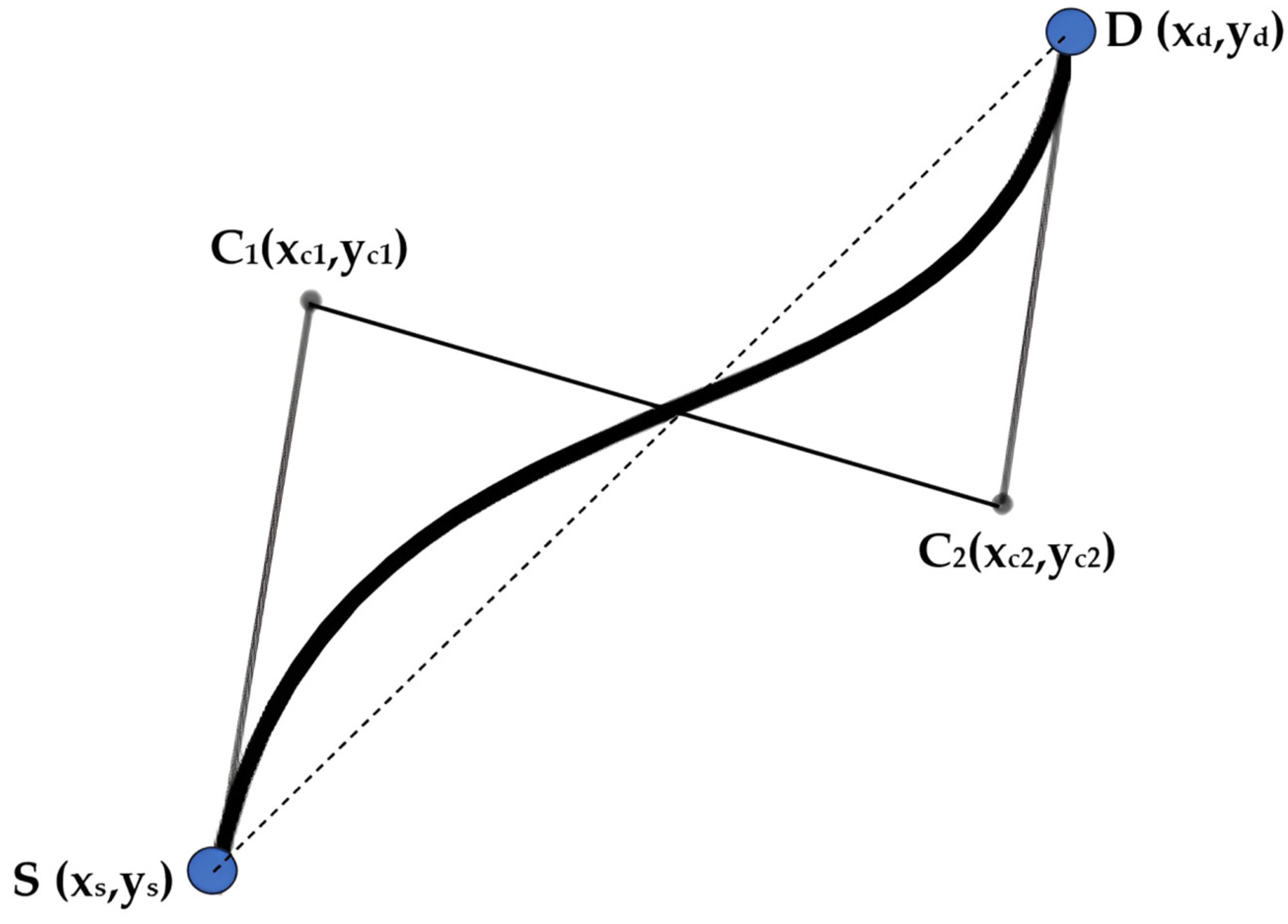
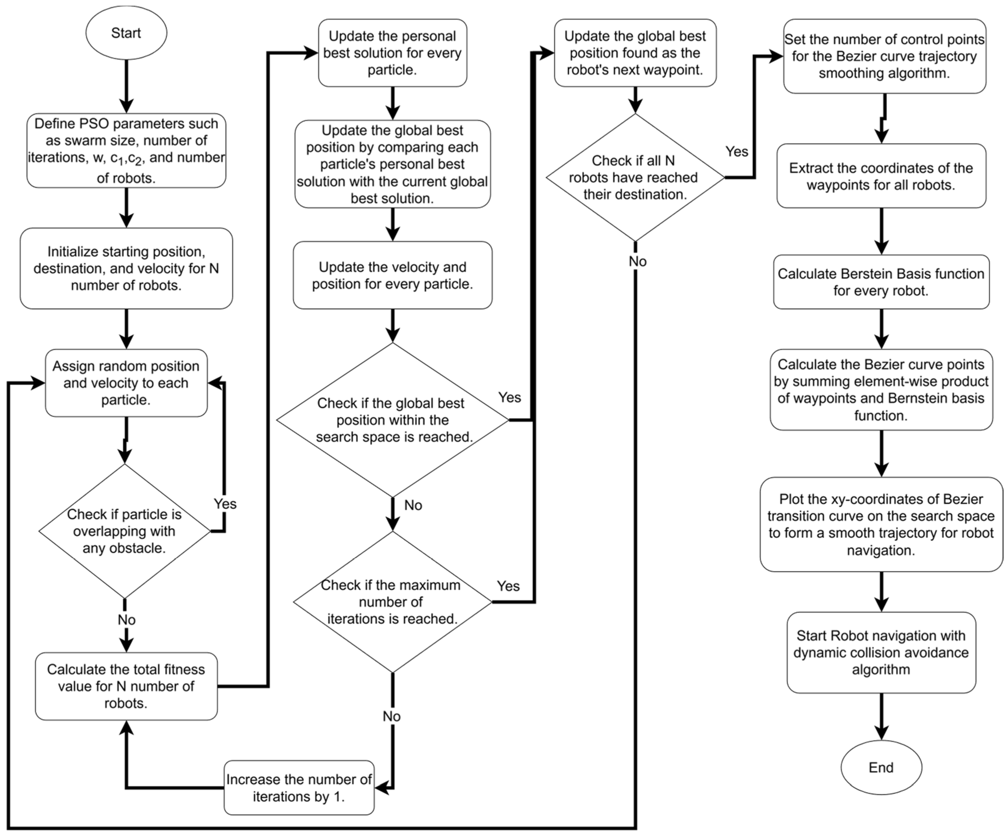
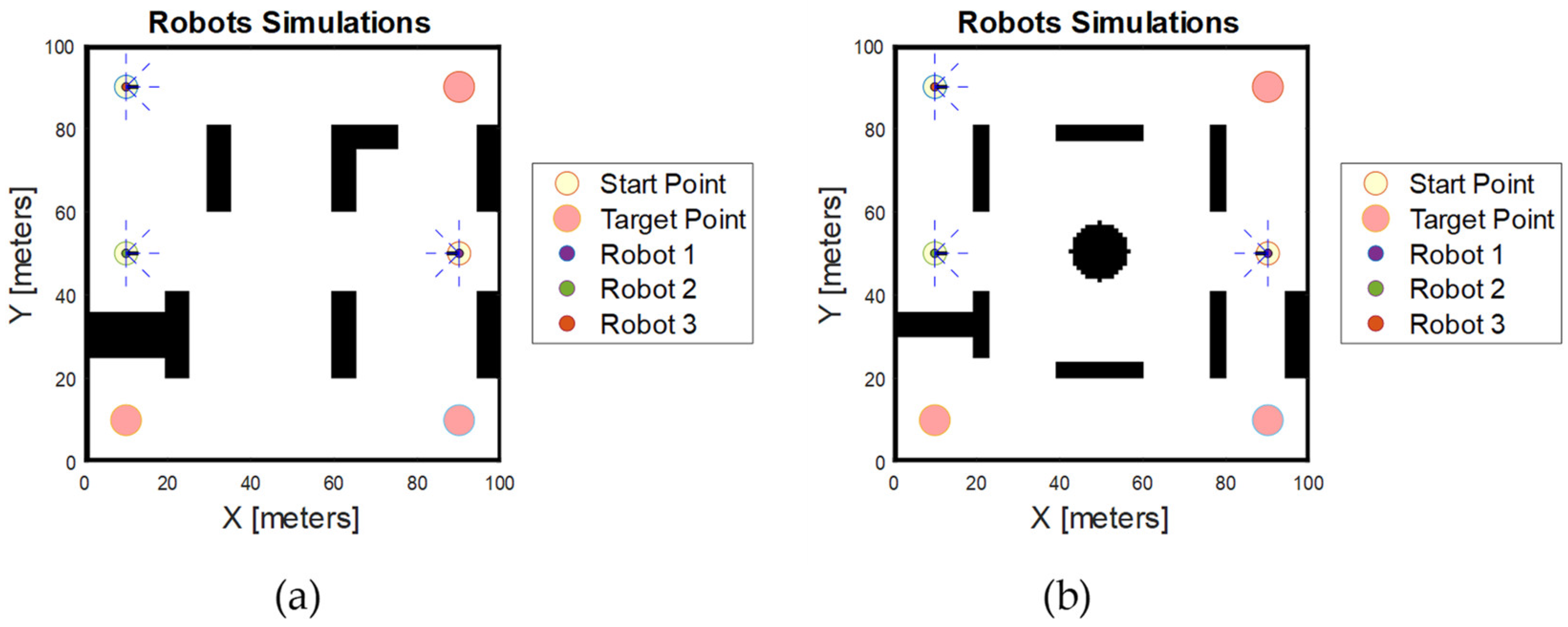
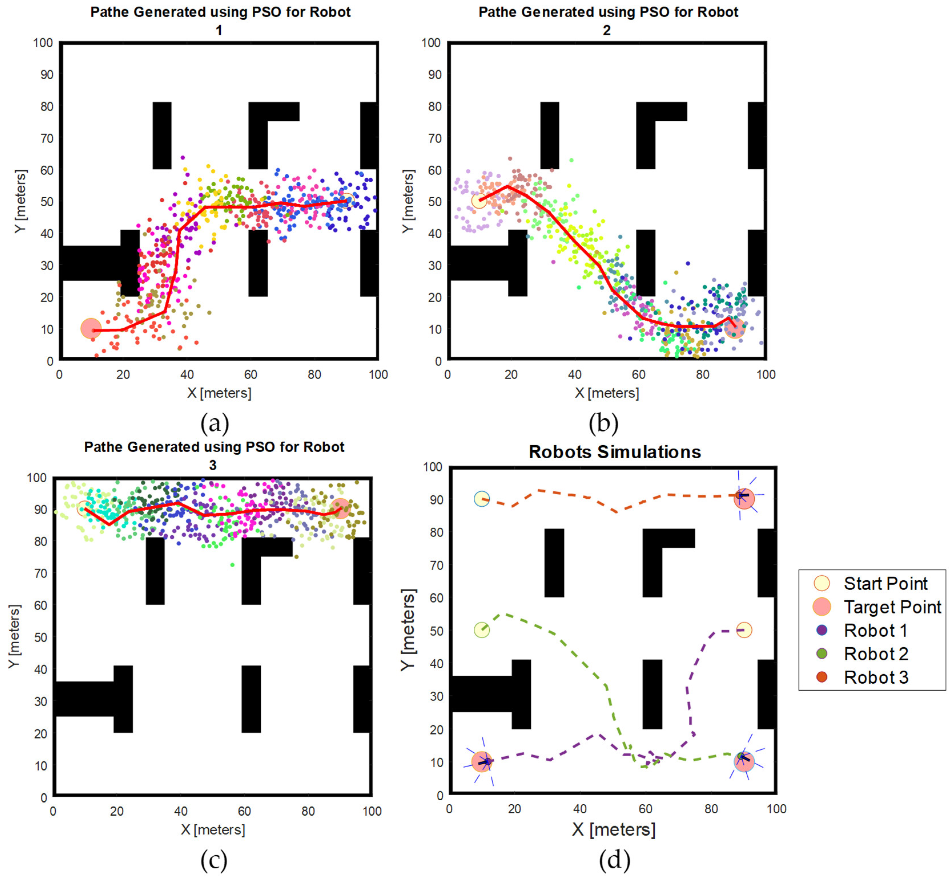
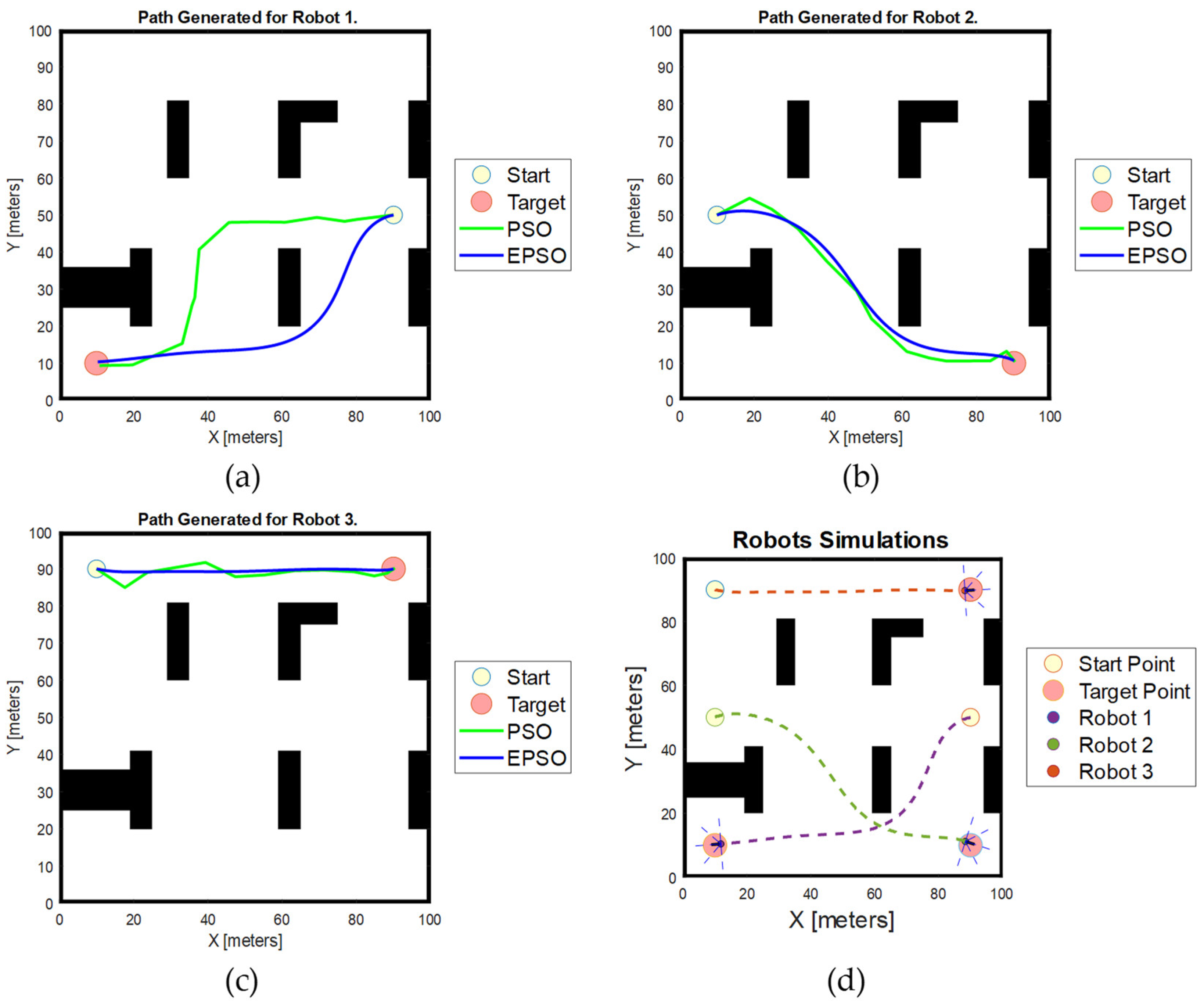

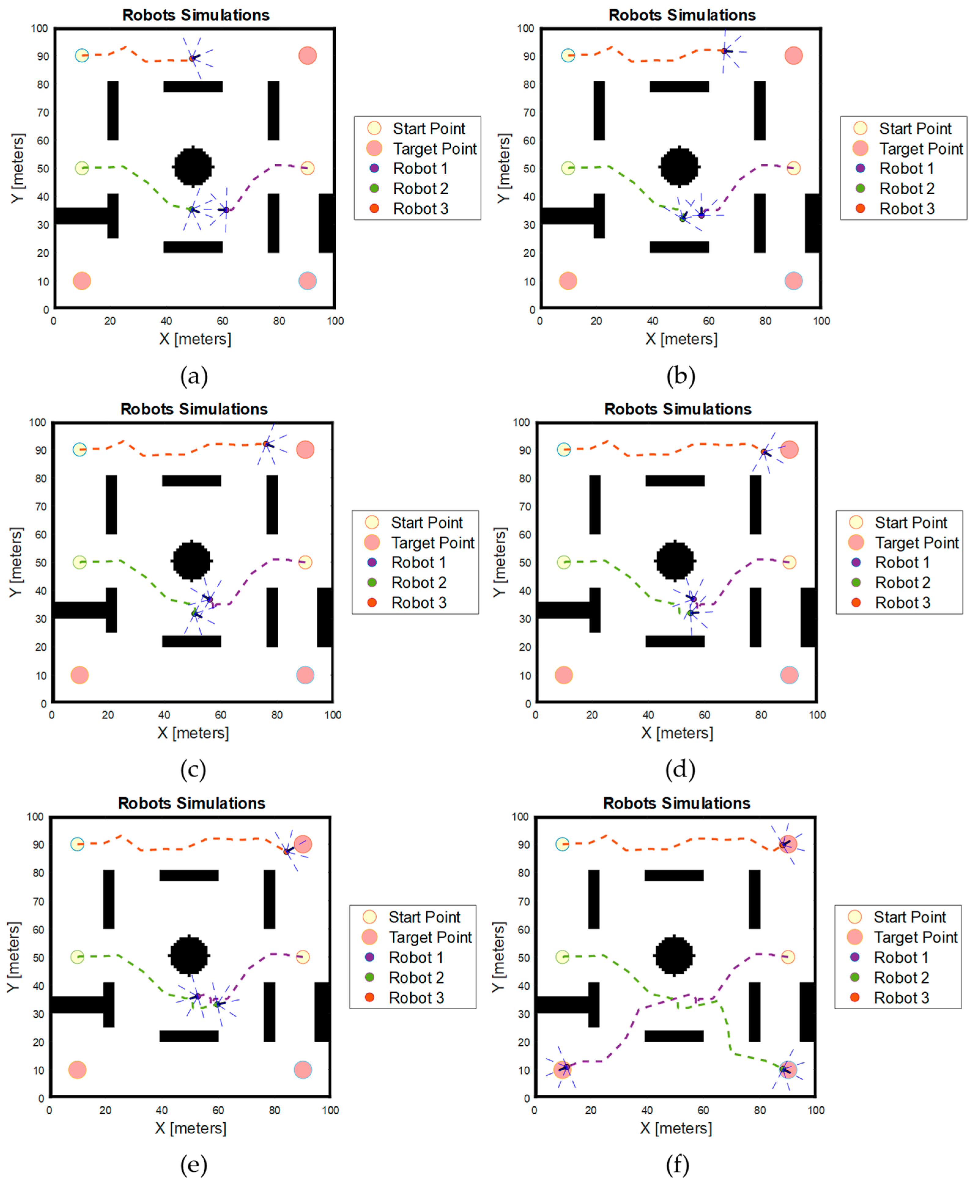
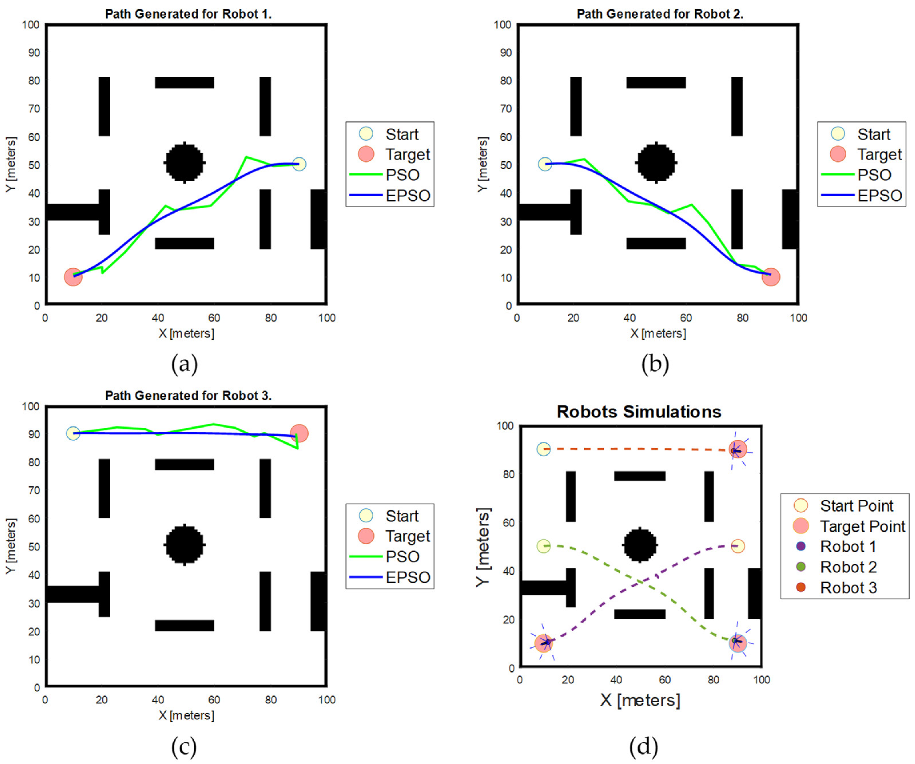
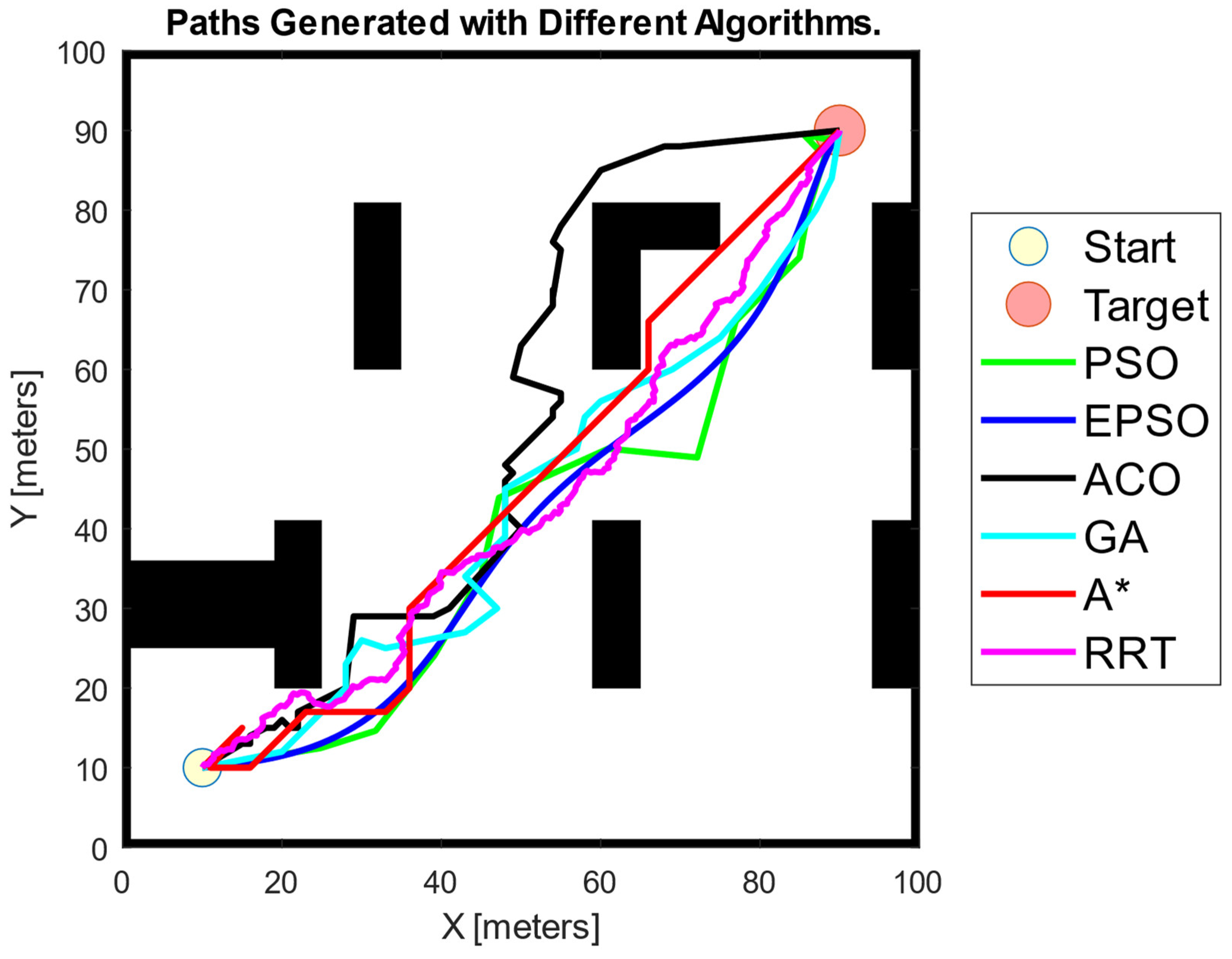
Disclaimer/Publisher’s Note: The statements, opinions and data contained in all publications are solely those of the individual author(s) and contributor(s) and not of MDPI and/or the editor(s). MDPI and/or the editor(s) disclaim responsibility for any injury to people or property resulting from any ideas, methods, instructions or products referred to in the content. |
© 2024 by the authors. Licensee MDPI, Basel, Switzerland. This article is an open access article distributed under the terms and conditions of the Creative Commons Attribution (CC BY) license (https://creativecommons.org/licenses/by/4.0/).