Abstract
The spherical shape is an interesting approach to develop exploration robots, or rovers, thanks to its capability of ensuring omnidirectional motion and of being basically unsensitive to possible rollovers. This works intends to propose a novel detailed design for such a kind of robot and to discuss the performance that can be reached by adopting this solution. The work hence introduces the requirements assumed for the design of the robot and discloses the general layout that was selected, which includes a pendulum for motion transmission and two coupled gyroscopes to overcome high, steep obstacles, such as steps. The paper then summarizes the functional design computation carried out to size and selects the components of the system. Eventually, a control algorithm is described and tested on a complete multibody model of the robot. The results in the execution of standard maneuvers such as motion on a horizontal plane, as well as in the overcome of a step, are shown. The energetic balance of the rover is described, and some preliminary consideration about mission planning are reported in the final discussion.
1. Introduction
Spherical robots (SRs) are highly advantageous in mobile robotics due to their protective spherical shell, preventing contamination and collisions. Their symmetrical design prevents overturning, allowing for falls and obstacle traversal without damage. The spherical shape facilitates energy-efficient rolling on slopes. Additionally, depending on the driving mechanism, SRs can achieve omnidirectional movements. These characteristics make SRs suitable for diverse applications, including exploration of unstructured environments, disaster area assessment, search and rescue operations, underwater inspection, surveillance, and more.
In the literature, many examples of SRs can be found. However, performances depend on the motion principle and on the mechanism employed to achieve it. One of the most common motion principles is the Barycenter Offset (BO). In such systems, the sphere hosts an internal mechanism that moves the barycenter from the equilibrium point so to create a driving torque. The advantage is that the locomotion system can be entirely embedded in the spherical shell, so to create a sealed environment. However, this results in a limited driving torque, as the amount of the offset that can be reached is constrained within the sphere radius. This also affect the capability to climb inclines and overcome obstacles, such as steps.
One way to exploit the advantages of BO and to overcome the limitations against obstacles is to combine it with auxiliary systems based on a different physical principle that increases the driving torque. For example, Control Moment Gyroscope (CMG) systems use the gyroscopic torque that is generated by tilting the axis of a flywheel rotating with high speed, which depends on the angular momentum.
This paper presents the design, modelling and control of a hybrid BO-CMG spherical robot intended for planetary exploration. The robot represents an important step forward with respect to the first prototype, described in [1]. The old version was based on a single-pendulum activated by a differential mechanism to realize BO. The new version improves the previous one by mounting a CMG on the pendulum.
The application of the single pendulum-CMG mechanism has some technical challenges. The spherical robot had a diameter of 0.5 m and a mass of 22 kg, so that it could be carried by hand. Fitting the hybrid mechanism within such a compact size required an iterative design, which considered the actual space available inside the shell and the desired performance of the CMG.
The design of the robot is supported by mathematical models of the subsystems, like gyroscopes, pendulum and transmission, and by multibody simulation. The result is a SR that, on the Earth, can run up to 2.5 m/s, climb slopes of 15° and overcome steps that are 10 times higher with respect to the previous version, which means steps up to 100 mm.
In the next section, an insightful review of existing SRs is presented in order to highlight the novelties of this work with respect to the state of the art.
1.1. Spherical Robots: State of the Art
Spherical robots can be classified based on the driving mechanisms developed so far [2,3]. The most common methods are BO and Shape Transformation (ST). Other propulsion strategies found in the literature include CMG, Reaction Wheels (RW), Wind Driven (WD) and Jet Propelled (JP). Each of the driving mechanisms will be covered in the following paragraphs, explaining their function and providing examples, with special focus on BO and CMG, as they are at the base of the robot presented in this work.
1.1.1. Barycenter Offset
The BO method involves an internal system that moves the barycenter of the SR, generating an eccentric torque that causes the robot to roll towards the barycenter position. This locomotion strategy enables movement on flat surfaces, overcoming small obstacles and climbing gentle slopes. One of the most common mechanisms for realizing BO is a pendulum with 2 Degrees of Freedom (DOF) hanging from a diametral shaft. The 2 DOF enable the swing of the pendulum about pitch and roll axes of the robot, so to generate rectilinear paths or curves as needed. Design and control are relatively simple, as the rotational axes of the pendulum can be actuated by compact electric motors. The main disadvantages are the lack of omnidirectionality and the limited torque.
A first example of a pendulum spherical robot is the GroundBot from Rotundus AB [4]. Boasting a diameter of 0.6 m and a speed of 3 m/s, it is equipped with cameras for surveillance, and it can autonomously patrol predefined routes via GPS. Despite its stability and robustness, GroundBot encounters challenges in obstacle traversal due to its propulsion mechanism’s limitations [5].
Researchers have proposed enhancements such as modifying pendulum structures and incorporating extendable pods for improved performance [6,7]. Innovations like Visionbot [8] and multi-mode motion designs [9] expand the capabilities of pendulum-based spherical robots. However, most of them utilize a single pendulum system, yet a few employ double pendulum configurations to enable quasi omni-directionality by turning in place [10,11].
A different manner to exploit BO consists of a multi/single wheeled mobile robot, placed inside the spherical shell and usually referred to as Internal Driving Units (IDUs), or Hamster-Balls (HB). HB robots offer compactness and enhanced torque, with recent HB designs featuring omni wheels for omnidirectional motion [12,13,14]. A simpler design based on classic wheels can provide both quasi-omni-directional and omnidirectional movements [15,16].
Alternative propulsion methods like the moving mass method enable omnidirectional movement with finer control over the barycenter position [17]. Finally, fluid-actuated spherical robots eliminate pendular instability, enabling precise forward and lateral movement [18]
1.1.2. Shape Transforming
A different class is represented by the shape transforming (ST) spherical robots. This class includes two groups that use two different propulsion strategies: the Shell Deformation (SD), which consists in deforming the spherical shape to generate a propulsive force, and the Hybrid Robots (HR), which can change their structure to change the propulsion method. The main advantage of being able to transform is the significant improvement in the ability to cross obstacles while retaining the advantages of the spherical shape. On the other hand, the mechanical design and control architecture of this type of robot are much more complicated.
SD may involve spherical deformation using inflatable sections, as in [19], or electroactive elastomer sections [20]. These robots benefit from softness, absorbing collisions, adapting to terrains, and ensuring safe interaction with humans. Hybrid robots, like those showcased in [21,22], combine rolling with walking or crawling, utilizing retractable legs or actuated mechanisms; such designs offer versatility in traversing various terrains and overcoming obstacles. A remarkable prototype by M. Zhang et al. [23] integrates rolling, crawling and flying capabilities, maximizing adaptability across diverse environments.
1.1.3. Angular Momentum
Some SRs exploit the angular momentum conservation principle to enhance their movement capabilities. Two possible strategies are used: the CMG, which consists in tilting a spinning rotor, and the reaction wheel (RW), which exploits the third Newton’s law.
CMG is based on the same principle used in spacecraft attitude control systems. A CMG array consists of one or more spinning rotors that can be tilted by one or more motorized gimbals; changing the orientation of the rotor spinning axes produces a gyroscopic torque which can be used to accelerate or change the heading of the spherical robot. Usually, two counter-rotating rotors are used, otherwise the tilting torque would cause the unwanted motion of the sphere. This drive mechanism is often used with another drive mechanism, such as BO.
An example of a spherical robot with a CMG drive system is the one developed by G. C. Schroll [24]. This robot uses two actuation mechanisms: the pendulum for forward and lateral movement, and a CMG group to provide greater torque to overcome to overcome steep slopes and obstacles. A similar example is proposed by [25], but with a double gimbal to solve the problem of desaturation, i.e., the gyroscopic torque decreases as the tilting angle increases. Another example is developed by J. Chen et al. [26], with the aim to use CMG to stabilize also the internal platform dedicated to sensors. Finally, a spherical robot with CMG array is the one proposed by H. W. Kim and S. Jung [27], characterized by three actuators: two are used to actuate two wheels in contact with the inner surface of the spherical shell that provide the driving force; a CMG actuator is used to control the heading angle (yaw).
On the other hand, the RW (Reaction Wheel) method employs spinning rotors to generate torques. However, it may suffer from unwanted gyroscopic precession, necessitating the flywheel to stop before changing the heading direction. For instance, the L.U.N.A. prototype [7] and the design by C. Li et al. [28] both utilize reaction wheels to enhance self-stability, despite challenges like high power consumption and control difficulties.
1.1.4. Other Spherical Robots
Other types of systems include robots powered by an internal drone, underwater spherical robots and wind-powered robots. For instance, a drone provides the cross-obstacle ability, while a spherical frame around it serves for protection and can be used for rolling as needed. The main disadvantage of this is the complicated control system. C. J. Dudley et al. presented a prototype of a micro spherical rolling and flying robot, that consists of a quadcopter encased in a lightweight spherical exoskeleton [29]. The Rollcopter by S. Sabet [30] uses six reversible propellers for controlled rolling and flying.
Underwater spherical robots, like MK-V and MK-VI from the University of Manchester, monitor nuclear storage tanks and wastewater treatment plants [31]. E.V. Potapov et al. presented the SUR IV model, capable of high-speed propulsion using propeller thrusters and low-speed propulsion using waterjet thrusters [32].
Wind-driven spherical robots explore large environments like deserts and polar regions; they feature low cost, low power consumption and a simple structure. Li T. and Liu W. [33] developed a collapsible wind-driven spherical robot for rolling, bouncing and flying. Team Tumbleweed’s wind-driven rover collects data from Mars [34], while Xie et al. integrated an internal pendulum for navigation in the absence of wind [35].
1.1.5. Contribution of This Work
This paper addresses the limitations of BO spherical robots with the proposal of a novel concept of hybrid BO-CMG propulsion system, based on a differential-driven single pendulum and a pair of flywheels. The differential-driven single pendulum can be seen as the primary locomotion system, while the CMG is denoted as the secondary locomotion system, which gives a torque boost when needed. The aim is to investigate design challenges and solutions to fit CMG within a pendulum-driven spherical robot and address the energy balance and control aspects related to the simultaneous actuation of pendulum and CMG when dealing with steps.
Similar solutions can be found in the literature. Some of them realize the same locomotion system but with a different design [24,26]; one has a different primary locomotion system [25].
The novelties of this work with respect to the literature can be summarized in the following points:
- An original design of the power transmission for a hybrid BO-CMG spherical robot.
- A method for the optimization of the size of the gyroscopes according to the specifications and the available volume in the shell.
- A control architecture with fuzzy gain scheduler for tracking straight trajectories.
2. Mission Specifications
The robot is thought of for the exploration of critical or uninhabited areas, and more generally, of planetary surfaces.
The list of specifications is reported in Table 1.

Table 1.
Spherical robot requirements.
The robot must navigate diverse terrains, resembling those found on Earth, Moon and Mars, where obstacles vary from rocky steps to inclined surfaces. Performance limitations stem from the assessments of the robot’s functionality. Remote control capability is essential, alongside provisions for battery power and recharging mechanisms. Lastly, the robot’s maximum size is constrained to ensure it remains portable for manual transportation.
The reason why the spherical shape is a viable solution for the mission specifications lies in it being able to create a robot that is immune to tipping and can withstand shocks, and to house sensor technology inside it that is protected by the shell. Furthermore, the ability to overcome obstacles such as steps puts it in a position to deal with uneven terrain. Last but not least, compactness: It will be demonstrated how it is possible to fit the locomotion mechanism inside the sphere, while still leaving space available for the sensors, which, depending on the mission, can measure temperature, pressure, humidity, radioactivity and gas data, and can provide images [1].
The compactness also lends itself to the possibility of storing the robot on a lander, thus opening up space exploration missions. In [1] for example, the possibility of using the robot for lunar applications was discussed. In this view, the dimensioning of the locomotion mechanism on the basis of Earth’s gravitational acceleration is a worst condition. This precautionary approach means that the robot can be used with even better performance against obstacles on Moon and Mars [1].
3. Functional Analysis of the Driving Mechanism
In the previous sections, the primary limitation of BO spherical robots was discussed: their restricted ability to overcome obstacles. To address this challenge, the potential of combining one or more Control Moment Gyroscopes (CMGs) as an auxiliary system is analyzed in this section.
3.1. Analysis of the BO Principle
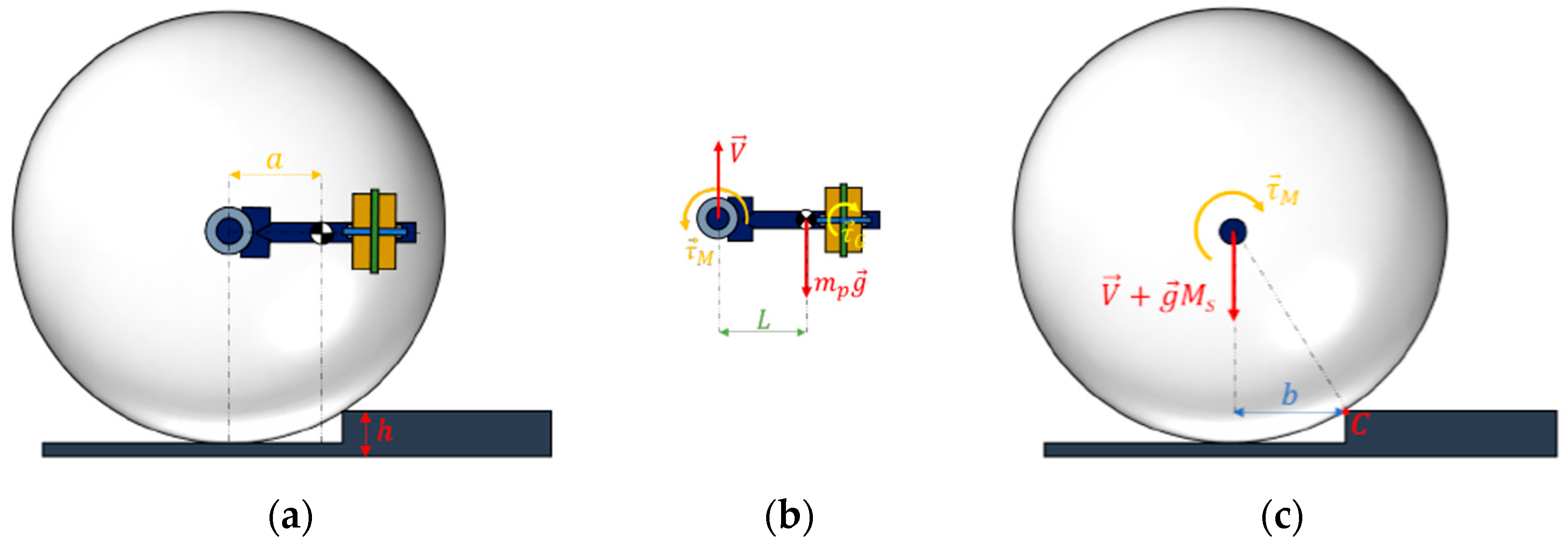
Consider a spherical robot on a flat surface with a pendulum hanging from a diametral shaft. In the rest configuration, the pendulum is vertical and the system is balanced; otherwise, the system is subjected to a driving torque due to gravity. For instance, when the pendulum is horizontal, the driving torque is maximized. By extending this reasoning to the cases of inclines and steps, it is possible to evaluate the spherical robot’s ability against obstacles. Two performance parameters, the Maximum Step Height (MSH), and the Maximum Slope Angle (MSA), can be introduced. These parameters are illustrated in Figure 1, with representing the MSH, and denoting MSA. In the same picture, the barycenters of spherical shell, pendulum and whole system are indicated with , and , respectively.
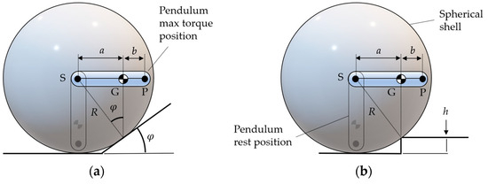
Figure 1.
Analysis of limit cases of incline (a) and step (b).
Let denote the distance between the barycenter of the system and the center of the sphere, and let denote the sphere’s radius. The following relationships can be written:
Increasing enhances the driving torque but also necessitates larger actuator sizes, which, consequently, affect the offset. In practice, for small spheres, the ratio can be roughly 0.5 [36]. The requirement of minimum slope Table 1 is easily satisfied. On the other hand, the minimum step of 0.1 m is unfeasible for a 0.5 m diameter sphere, as it would require a ratio. For example, the previous design of the same size achieved a 0.44 ratio with not a few challenges [1]. Hence the need to introduce an auxiliary system to increase the driving torque.
3.2. Analysis of the CMG Principle
CMG is a device that has been used in several applications, such as attitude control for space and stabilization for robotic systems. The purpose of this section is to recall the working principle of the CMG and to discuss its potential application to spherical robots.
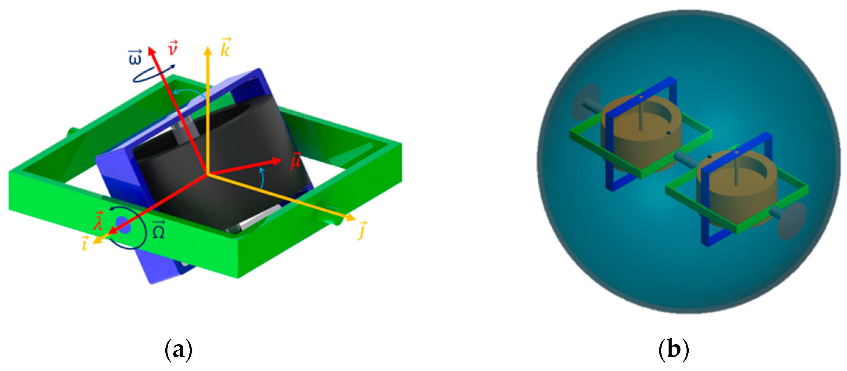
The most common version of CMG is the single gimbal configuration, which is shown in Figure 2a.

Figure 2.
(a) One gimbal CMG. (b) Scissored-pair CMG.
The reference system in yellow is fixed, while the red reference system is attached to the blue gimbal. The two reference systems are centered at the barycenter of the gyroscope, which spins about with a velocity , and that can be rotated about with a velocity . For such a system, the gyroscopic torque can be written as:
where is the moment of inertia with respect to the axis, and is the tilting angle with respect to the axis.
By assuming that is the rolling axis of a sphere, the component of is unwanted. Moreover, the tilting action would require an actuation torque, which would be a disturbance for the sphere. A solution can be achieved using a second CMG in such a way that the effect along the direction of interest is doubled, while the other component is canceled out. To do so, the two gyroscopes must have opposite and . When the gyroscopes are used in this configuration, they are also known as scissored-pair control moment gyroscopes. In Figure 2b a scissored-pair CMG is shown, mounted inside a spherical shell.
3.3. Combining BO and CMG
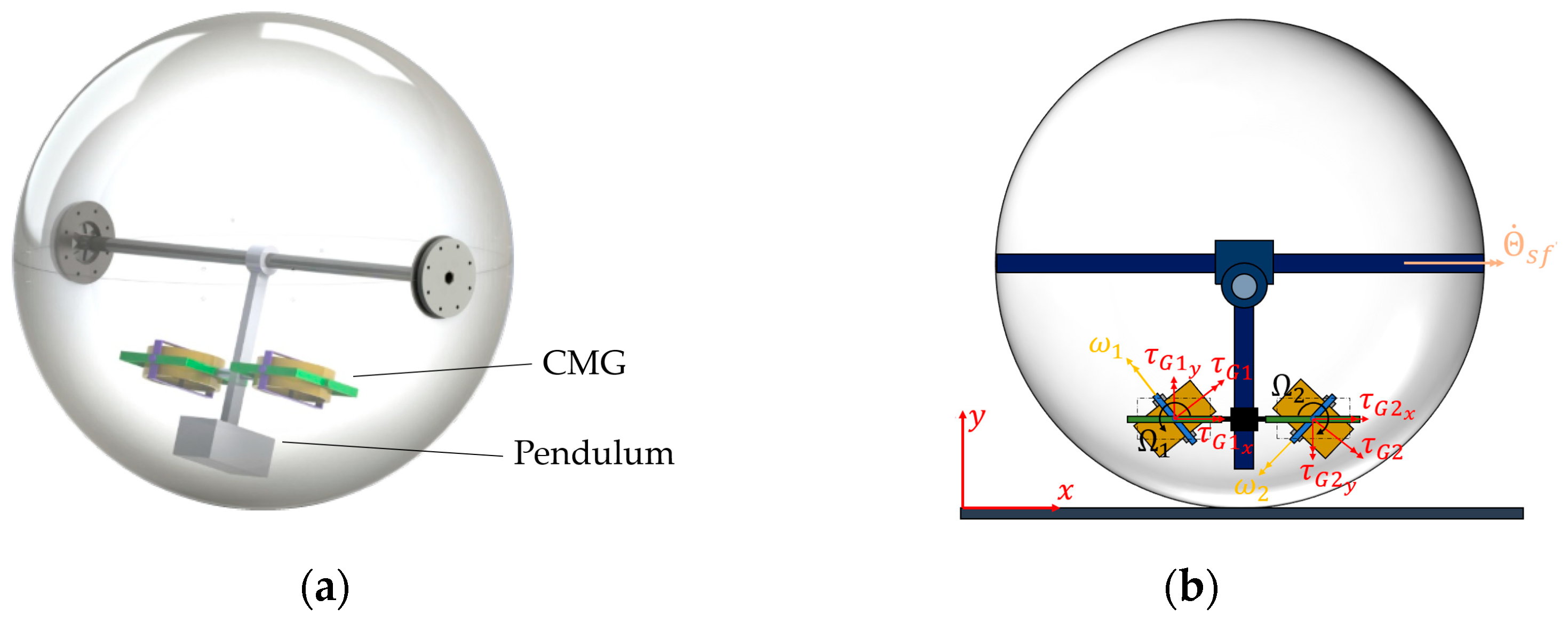
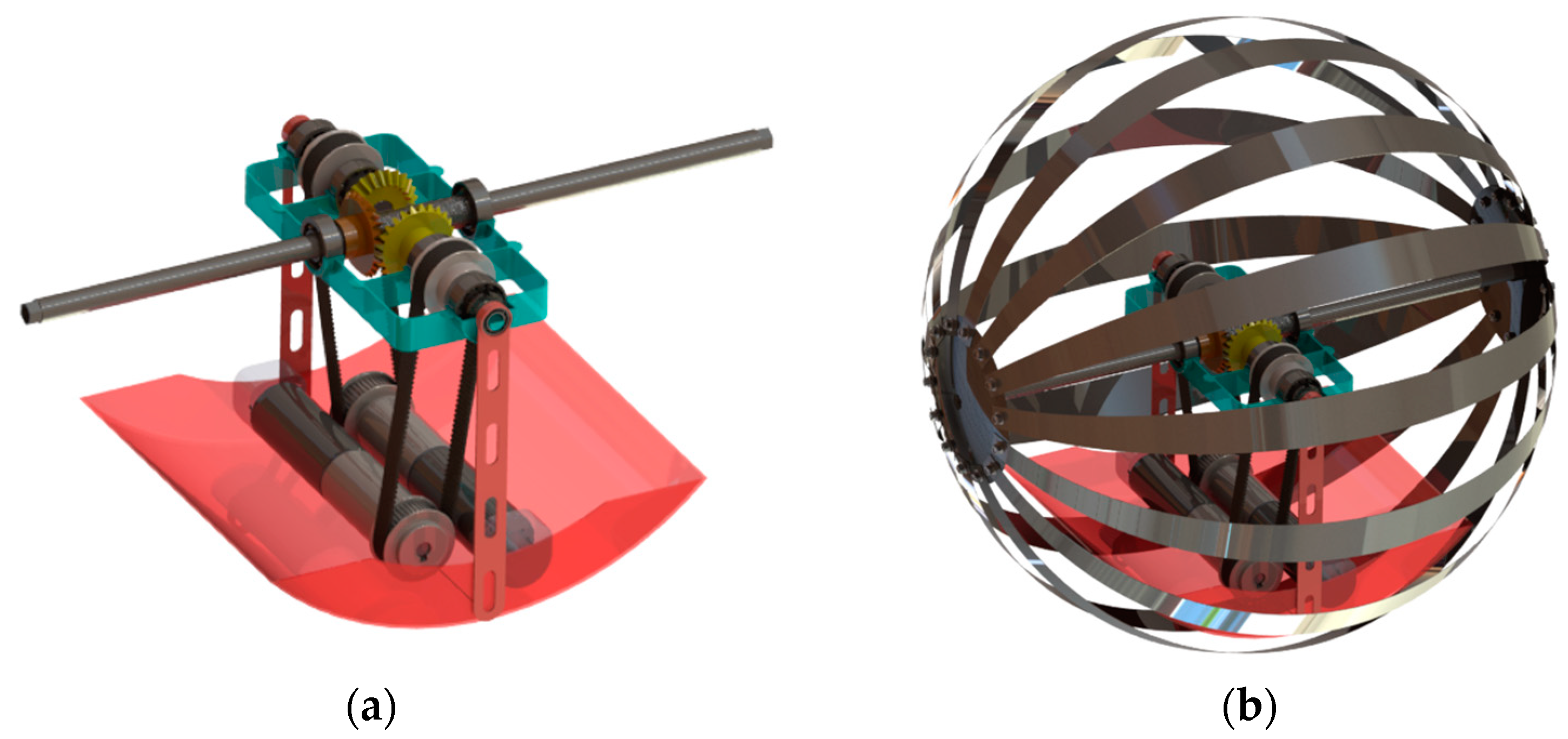
To exploit the gyroscopic torque, the idea is mounting a scissored-pair CMG on the pendulum, as shown in Figure 3. Whenever the robot requires a torque boost, the CMG can be activated and the gyroscopic torque is exerted to the pendulum.
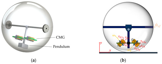
Figure 3.
(a) Conceptual design of a BO-CMG spherical robot. (b) Front view of CMG activated, with schematics of gyroscopic torque components.
Activation of CMG translates into increasing the pendulum’s weight instantaneously. Consequently, maintaining the pendulum at a 90° angle requires more torque by the actuators, which is then transferred to the sphere shell. The free body diagram in Figure 4 examines the static equilibrium of a sphere encountering a step.
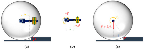
Figure 4.
Free body diagram of the robot while climbing a step (static equilibrium condition). (a) system; (b) pendulum; (c) spherical shell.
The problem can be divided into two parts: analyzing the forces acting on the pendulum and analyzing those acting on the sphere. The equations obtained are as follows:
where is the total torque provided by the motors, is the gyroscopic torque component of the scissored pair about the rolling axis, is the spherical shell mass, the pendulum mass, is the distance between the barycenter of the pendulum and the center of the sphere and is the constraint force.
Rearranging these equations, it is possible to recalculate the MSH-over-radius curve while including the effect of the gyroscopic torque:
Comparing Equation (1) and Equation (4), it can be observed that is increased by a factor that depends on the gyroscopic torque and the total mass of the system. In Equation (4), a new variable, , is defined as:
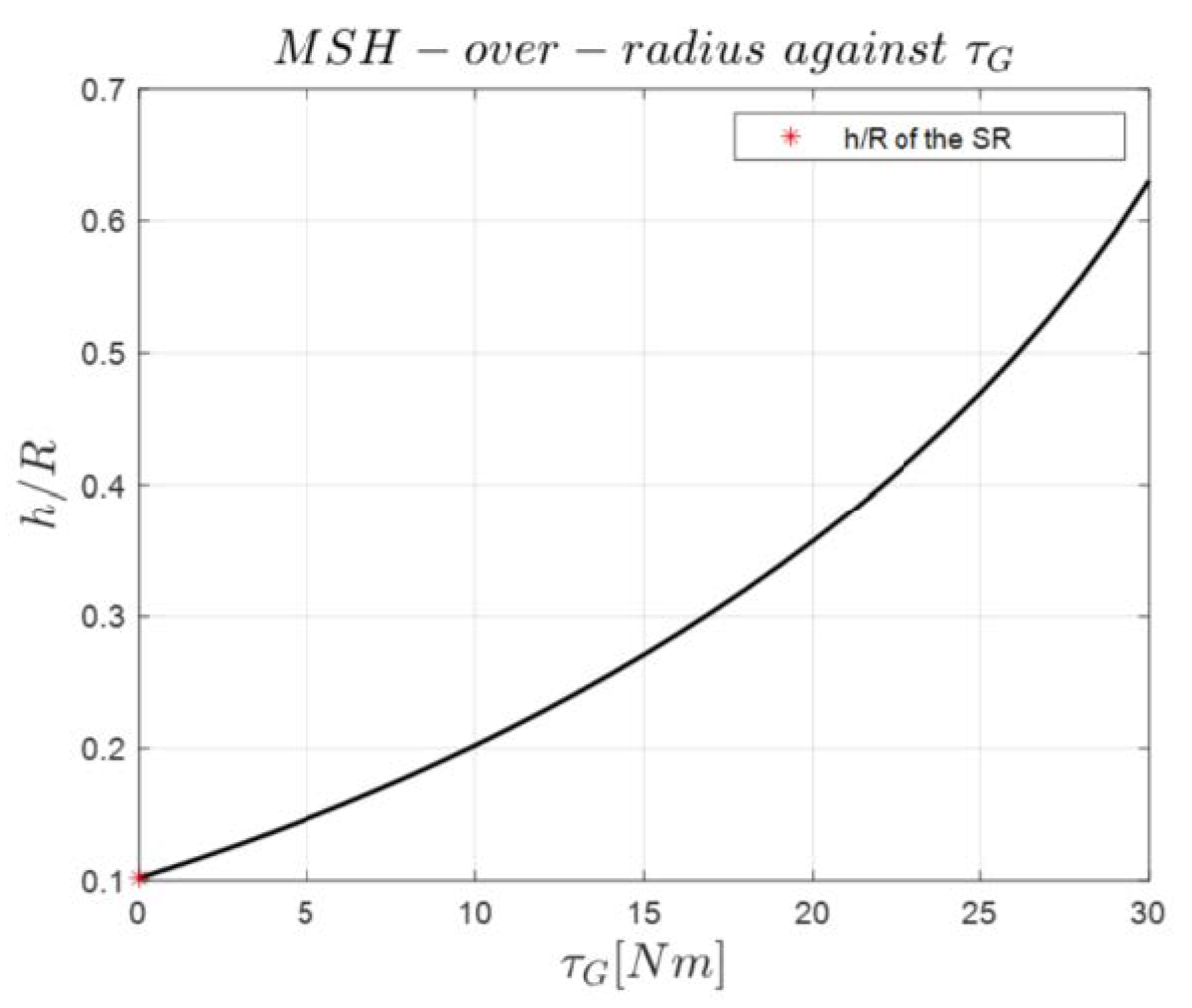
To understand how the maximum step height can vary with the aid of the gyroscopic torque, the new relation between the step over radius and the maximum gyroscopic torque expressed by Equation (4) is represented in Figure 5.
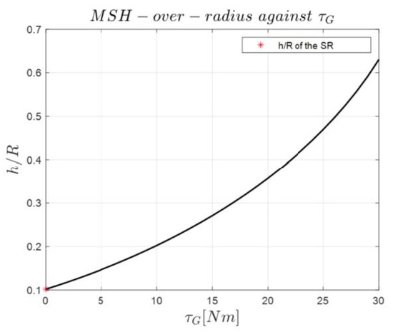
Figure 5.
MSH-over-radius curve against Maximum Gyroscopic Torque. Total mass and barycenter position of the robot from [1].
Without gyroscopes, step height is a 10th of the radius, as noted in [1]. In Figure 5 is considered , as this is the initial condition. However, the gyroscopic torque’s useful part changes with tilt angle, as from Equation (2). As the gyroscopes tilt, the effective distance decreases until it matches the initial value . Yet, the torque for climbing a step decreases as the robot ascends. Also, is not solely determined by gyroscopic torque but also by the system’s total mass.
4. Design
4.1. Overview of the Previous Design Based on 2-DOF Pendulum
The primary propulsion system is the 2-DOF pendulum. The design of the pendulum mechanism is kept similar to [1] and is shown in Figure 6. Unlike traditional designs, the pendulum actuators are not directly attached to the central shaft. Instead, they are placed at the pendulum base to lower the robot’s center of gravity. Motion is transmitted to a differential driving system at the shaft center via two belts. This system includes a single planet gear on the shaft and two sun gears connected to motors with timing belt.

Figure 6.
(a) Driving mechanism and pendulum. (b) Assembly of the SR with the layer of harmonic steel sheets [1].
The spherical shell consisted of two layers, namely the inner layer made of harmonic steel sheets bent to assume a spherical shape, and the outer layer made of impermeable rubber. The combined mass of the spherical shell and the differential mechanism was approximately 5.7 kg. This value was used to determine the pendulum mass and the barycenter distance from the sphere center.
4.2. New Design Based on Pendulum-CMG Mechanism
To improve agility and counteract external disturbances, the CMG system is introduced. However, seamlessly integrating this system without altering the robot’s size is critical for maintaining compatibility and functionality. Therefore, the objective remains to add CMG while preserving the SR’s footprint and integrity.
4.2.1. Design of CMG
The design of the locomotion system begins with the dimensioning of the flywheel, highlighting the procedure that was followed to define its size based on the design specifications. Subsequently, the selection process for the spinning motors is presented. Finally, the design of the gyroscope is presented.
- Flywheel Dimensioning
The dimensions of the flywheel are established through an analysis of the maximum gyroscopic torque. From Equation (4):
The step height (MSH) was set to be 110 mm. The spherical radius and the barycenter position are determined based on the design specifications: and . Subsequently, the influence of the system mass on the gyroscopic torque was investigated. The system’s mass leads to a decrease in the required gyroscopic torque. Various options are explored, ultimately leading to the determination that the minimum achievable mass was . From this total mass, the pendulum contributed , while the sphere and differential mechanism together accounted for 6 kg. Consequently, the resulting maximum gyroscopic torque was determined to be .
This value was then used to compute the inertia of the gyroscope flywheel. The spinning and tilting velocities were taken to equal to and , respectively. The flywheel inertia was taken to result in . Thus, one can write the following:
where is the steel density and the flywheel height.
The mass of the flywheel is assumed to be . Two equations alone can not determine its size. Fixing one variable might find a solution but may not maximize internal space use. Hence, a nonlinear constrained optimization problem aimed to minimize flywheel dimensions. The problem’s variables are , , . The function to minimize is distance from the cylinder’s edge to its center:
In addition to constraints Equations (7) and (8), a linear inequality constraint can be defined, which limits the external radius to :
The flywheel sizes from problem solution are reported in Table 2; the final design is then slightly adjusted due to initial hollow cylinder approximation.
Table 2.
Sizes of the flywheel.
- Drag forces on a high-speed spinning flywheel
In order to size motors for the flywheel’s rotation, accounting for potential high-speed rotor losses due to aerodynamic forces is critical. Typically, reducing drag involves housing the flywheel and lowering inner pressure with a vacuum pump. However, this is not viable for the spherical rover, nor would the occasional use of gyroscopes suggest this solution. The Von Karman-corrected formula was considered to estimate the drag torque [37]:
where R is the radius of the flywheel, l its thickness, ρa air density, ω angular velocity and drag torque coefficient ( if , if ). Table 3 reports the data used for the drag torque computation.
Table 3.
Values considered for drag torque computation.
The computed drag torque is 42 mNm. A safety coefficient of 1.25 was considered and, so, a drag torque of 52.5 mNm was assumed as the reference for the purpose of motor sizing.
- Spinning motors
The motor selection process focused on three main criteria: torque, speed and voltage. It was crucial to ensure that the motor’s torque exceeded air friction torque at maximum velocity. The obtained result was 52 Nm. The nominal speed was fixed when designing the flywheel at 8000 rpm. As for the nominal torque, the value used for the motor choice has been divided by a safety factor of 0.95, obtaining a speed of approximately 8420 rpm. A nominal voltage close to was desired, with Maxon’s tools confirming the motor’s suitability within the required operating range, along with voltage and current requirements of about and , respectively. Following thorough analysis, a fitting motor was discovered in the Maxon catalogue: the DCX 35 L, a graphite-brushed DC motor.
- Gyroscope assembly
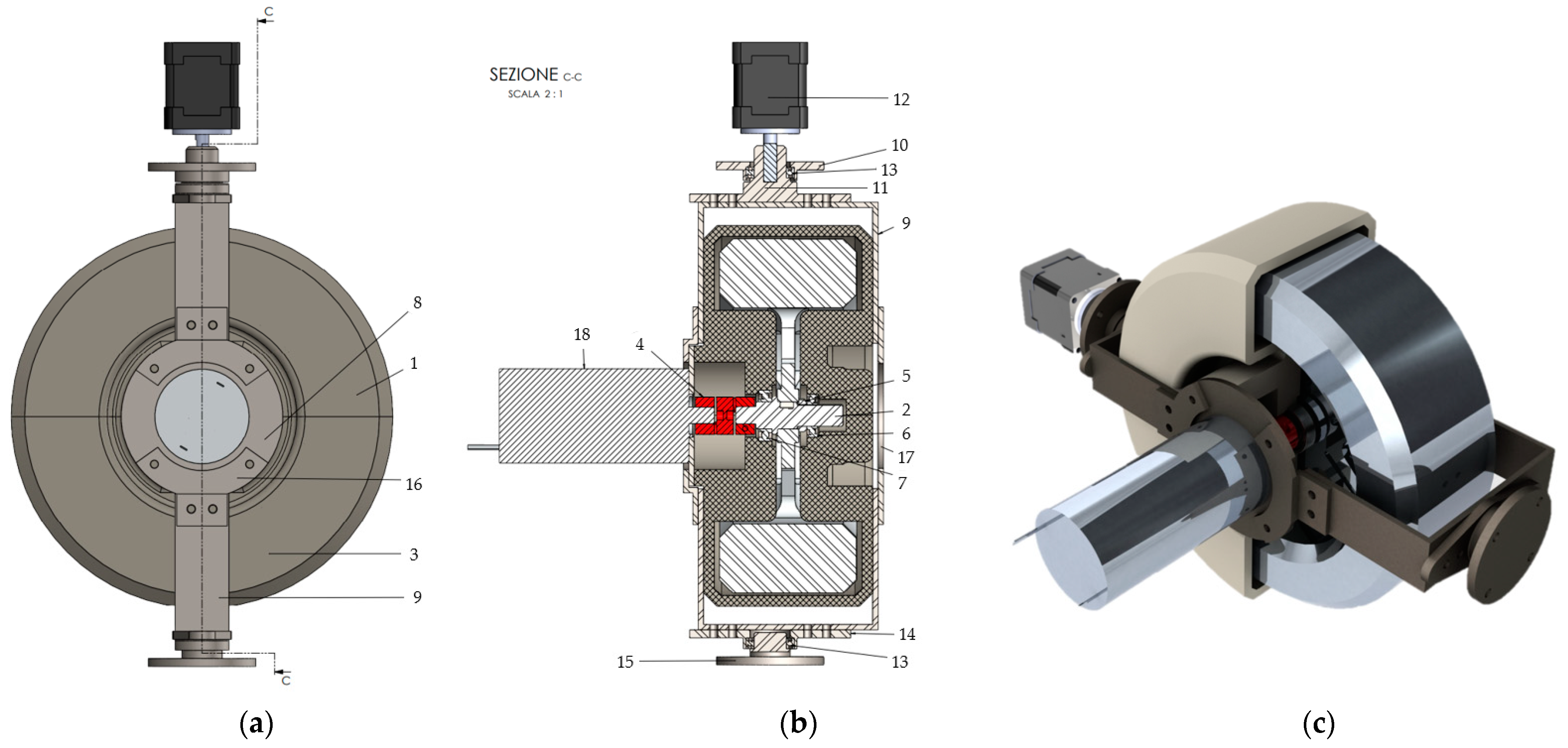
The gyroscopic group consists of the flywheel and its associated motors. The system’s design is depicted in Figure 7, showing a front view and a lateral cross-section. A jaw coupling connects the motor to the shaft. The gyro case provides structural support and user safety, minimizing drag friction. It is split into two halves for easy assembly, connected by screws and plates. The tilting motor axis aligns vertically with the system’s center of mass, allowing for a smaller motor (QMot QSH2818). Connectors (elements 10 and 15) bear the system’s weight, reducing shear load on the stepper motor shaft.
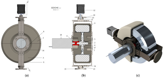
Figure 7.
(a) Front view of the gyroscope system; (b) cross-section; (c) 3D of the assembly. (1) First half of the case, (2) shaft, (3) second half of the case, (4) jaw coupling, (5) spacer, (6) small angular contact ball bearing, (7) big angular contact ball bearing, (8) motor plate, (9) C-plate for tilting motor connection, (10) flange1 for main structure connection, (11) flange1 for tilting motor-gyroscope connection, (12) tilting motor, (13) angular contact ball bearings for tilting axis positioning, (14) flange2 for tilting motor-gyroscope connection, (15) flange2 for main structure connection, (16) motor-to-C-plate connection plate, (17) closing Plate and (18) Spinning Motor.
4.2.2. Pendulum Actuators
The introduction of CMG changes the mass distribution of the pendulum and increases the power needs of actuators. The process to estimate the new size of differential drive motors is similar to [1] and considered the required nominal speed for climbing a slope. In such case, the motors provide the torque to maintain the pendulum at the equilibrium angle , i.e., where the robot’s barycenter aligns vertically with the contact point between the shell and ground. Consequently, the resultant continuous power output from the gearbox of the single actuator is derived as:
where and are the differential and toothed belt transmission efficiencies, respectively. Moreover, because of the CMG, the gearbox must withstand a maximum torque , which is determined by halving the combined torque needed to elevate the pendulum to a 90° angle and by adding the maximum gyroscopic torque.
Table 4 provides insight into the data used for motor and gearbox selection. Gearbox selection focused on meeting nominal and maximum torque requirements. Gear ratio was optimized to match the allowable ratio, minimizing torque demand on the motor. At the end, the Planetary RE 40 motor combined with Gearhead GP 42 C was selected from the Maxon catalogue.
Table 4.
Data used to design the main motors.
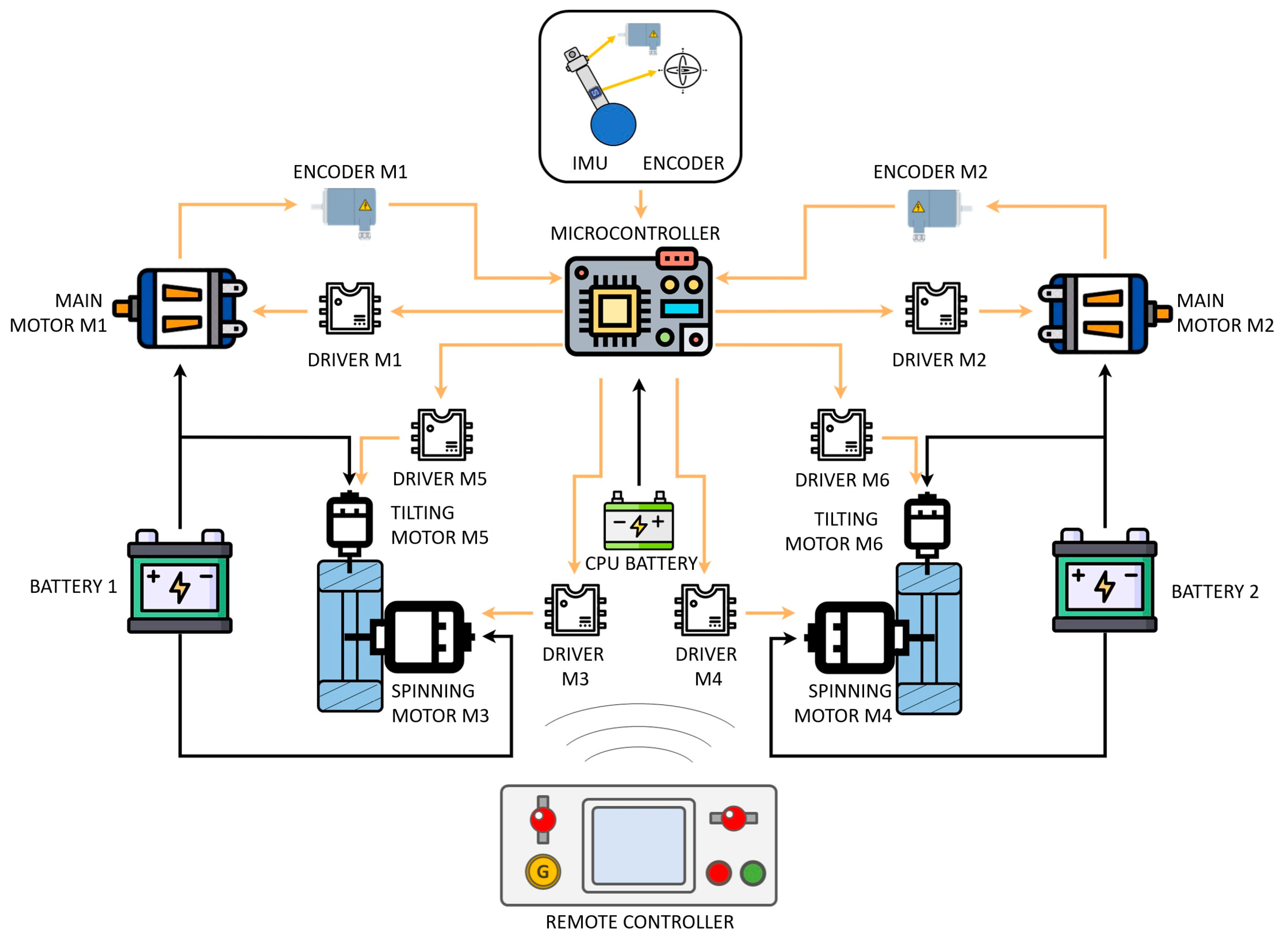
4.2.3. Electrical Integration
The hardware configuration of the SR encompasses a comprehensive set of components, shown in Figure 8. A microcontroller drives the execution of tasks and coordinates the interplay between different hardware modules. “Main motor 1” and “Main motor 2” are the two motors responsible for controlling the orientation of pendulum. Motors 3 and 4 are the ones responsible for the spinning motion of the gyroscope flywheels, while motors 5 and 6 are the ones used to perform the tilting movement. To ensure efficient operation and control of the motors, all of them are equipped with dedicated drivers.
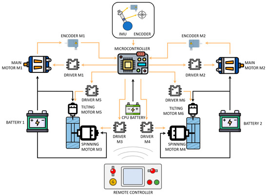
Figure 8.
Diagram of the hardware configuration.
For teleoperation, four kinds of sensors are essential: encoders for main motors, IMU for angular tracking, and an encoder for pendulum alignment. Power relies on two large batteries for motors and a smaller one for microcontroller and sensors. Batteries were carefully chosen for space, weight and runtime. A remote controller enables user interaction via radio or Wi-Fi.
- Battery dimensioning
Batteries were sized for a minimum 1 h runtime while climbing a slope at. Motor requirements were computed using torque and speed, resulting in a need for and . For a 1 h runtime, a battery with at least a capacity is necessary. The best option found is an Li-Ion battery pack with capacity and nominal voltage, meeting project needs.
- CMG impact on autonomy
The gyroscope’s motor significantly impacts battery life. By assessing the power needed for maximum velocity () with a input, current consumption over time is calculated. Integrating this gives the total charge consumed; one minute consumes about of a battery’s capacity.
During a gyroscope-assisted maneuver, the primary motors play a crucial role in counterbalancing the gyroscopic torque to stabilize the pendulum and transfer torque to the sphere. The maximum torque required by the motors is the amount necessary to sustain the pendulum in a raised position at a angle throughout the entire maneuver. In paragraph 4, the maximum gyroscopic torque was evaluated, resulting in . The torque required to raise the pendulum to a angle can be calculated using Equation (24), yielding . Therefore, the total torque required by each of the main motors is:
where while is the tilting velocity of the gyroscope, set to Ω = 15 rpm. Integrating this equation over the time interval the total charge consumed is computed. The obtained result is approximately the of the total charge of a battery. Therefore, the total amount of charge consumed each time the gyroscope is used can reach up to a of the total charge of a battery.
4.3. Design Result and Considerations
The CAD model Figure 9 illustrates the design; though hardware components are not depicted, the design accounts for their space requirements.
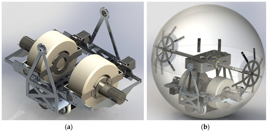
Figure 9.
(a) Rendering of pendulum and CMG; (b) final design of the spherical robot.
The pendulum structure of the spherical robot is crucial for functionality and stability, supporting the CMG group, main motors, batteries and hardware. Its design prioritizes structural integrity, weight optimization and compactness, using steel and aluminum alloy plates. Overcoming space limitations posed by the spherical shape was challenging, ensuring CMG rotation without interference and meeting barycenter placement requirements. The result is a lightweight pendulum frame structure (under ) for future upgrades. When placing the main motors and the CMG group, the total mass of the pendulum subsystem is about , with still available for batteries and hardware components. A rendering of the pendulum frame, actuators and CMG is shown in Figure 9a. A PMMA shell was used instead of the harmonic steel sheets of the SR from [1] because they were considered too flexible. A second layer made of impermeable rubber is needed to enhance the static friction of the shell on the ground, like in [1]. The total mass of the model is approximately , where the pendulum accounts for .
In Table 5 the properties of the final design are listed. These specifications make the SR able to climb a step with a height of 110 mm. This value was chosen in order to satisfy the MSH design requirement of 100 mm. From a theoretical point of view, it can be verified that these values are correct, using the equation Equation (5). In particular, the value of results in being equal to 0.8285. The corresponding value is equal to 0.44, which, when multiplied by the radius, gives a MSH of 110 mm.
Table 5.
Final design parameters of the spherical robot.
5. Modelling and Control
5.1. Two-Dimensional Analytical Model
The subsequent chapter focuses on the analysis of the two-dimensional analytical model of the robot rolling along a straight path. The model plays a pivotal role in investigating the robot’s response to varying inputs and to design and test the control strategy, which aims to track the spherical robot’s reference speed along a straight path.
5.1.1. Two-Dimensional Kinematics
The problem of the robot moving along straight path is represented through a schematic illustration in Figure 10. The system can be described through two generalized variables: the angle of rotation of the sphere computed from the starting position (q1), and the lifting angle of the pendulum measured from the line perpendicular to the inclined plane (q2).
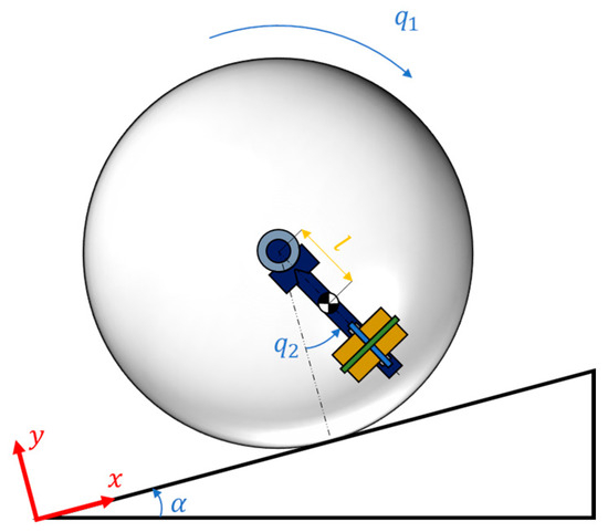
Figure 10.
Two-dimensional representation of the robot climbing a slope. q1 and q2 are the generalized variables.
Considering a fixed reference system with the x-axis parallel to the inclined plane, the robot’s x-coordinate can be defined under the assumption of pure rolling as:
Therefore, the position and linear velocity, as well as the rotational velocity of the sphere can be described as:
The pendulum is attached to the center of the sphere, and it can be approximated as a point mass with a constant distance from the sphere center equal to l. Its position depends on the sphere center position and on the lifting-angle described by q2. The equations describing the pendulum kinematics are the following ones:
where ci and si are the cosine and the sine of the generalized variable qi, respectively.
5.1.2. Two-Dimensional Dynamics
The dynamic model is obtained through the Lagrangian Approach. The Lagrangian function is defined as:
where K and P are the total kinetic and potential energy of the system, respectively. This function is used to obtain the n differential equations describing the problem, where n is the number of generalized coordinates. In this case, two generalized coordinates have been used; therefore, two differential equations are sufficient to describe the problem. Their form is the following one:
where are the generalized forces, non-conservative forces acting along the i-th coordinate.
The total kinetic energy of the system composed by the sphere and the pendulum is computed as:
where m and M are the pendulum and sphere masses, respectively; I is the total inertia of the sphere, while Ip is the total inertia of the pendulum.
The potential energy of the system is described by the following equation:
where the gravitational acceleration vector is expressed in the fixed reference system of:
These equations can be used to obtain the n differential equations describing the problem:
where τM is the motor torque, and are the torques due to external non-conservative forces, In is equal to:
Under the assumption of pure rolling, and by neglecting the rolling friction, non-conservative forces are null. However, some dissipation is considered through viscous friction coefficients β1 and β2.
These equations do not account for the effect of the gyroscopic torque, because they were used to study the straight-line movement of the robot, but it could be included by subtracting the gyroscopic torque in the right-hand side of the second equation.
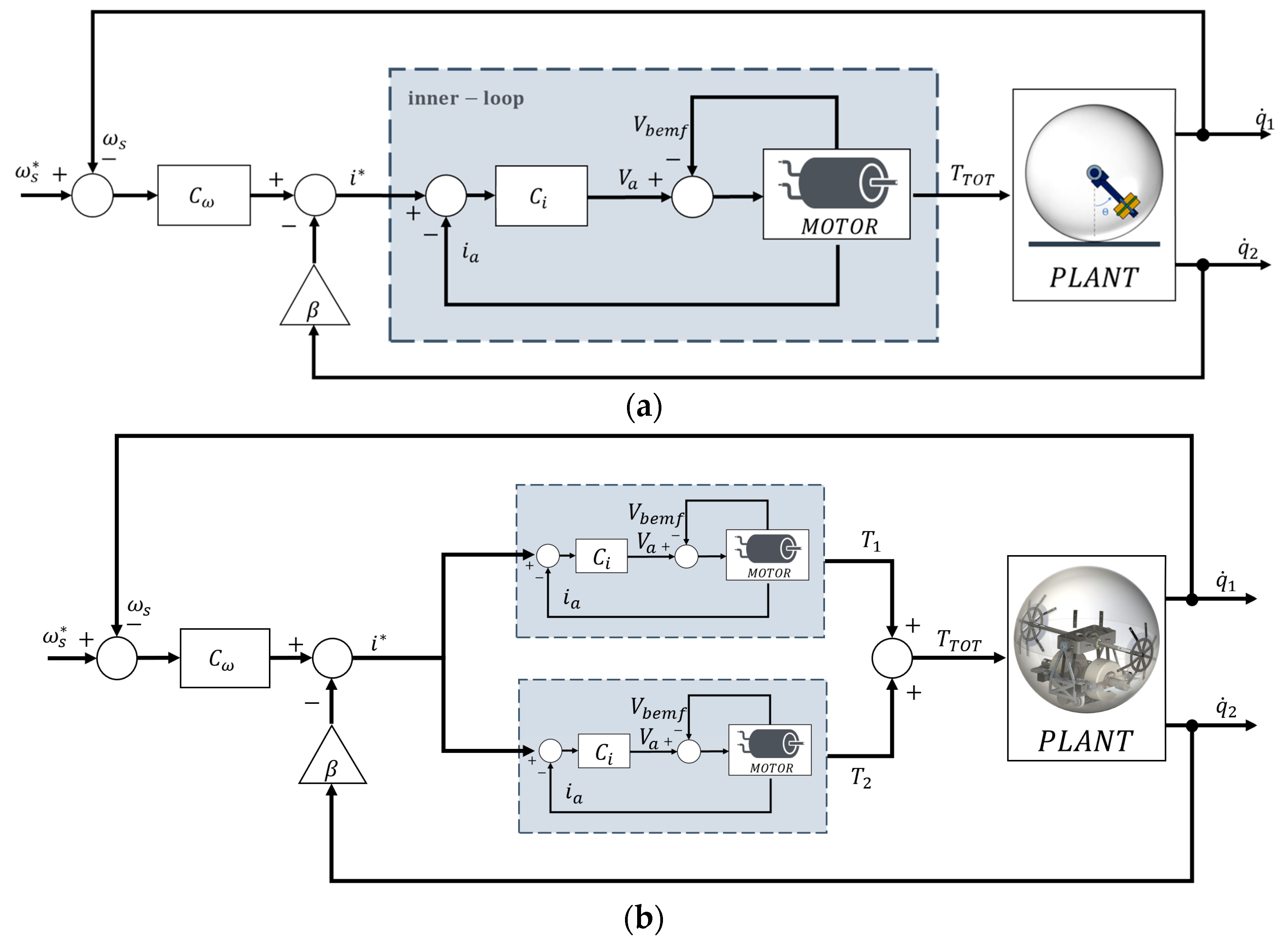
5.2. Straight-Trajectory Control Strategy
The controller aims to track accurately the spherical robot’s reference speed along a straight path. It is characterized by two control loops: an external loop and an inner loop (Figure 11a). The external loop is tasked with determining the input to the pendulum motor based on the angular velocity error of the robot, whereas the inner loop is focused on regulating the motor speed.
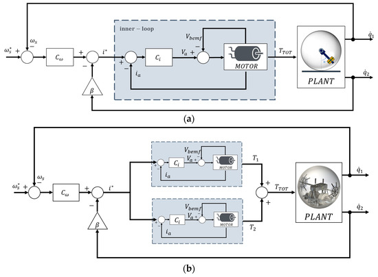
Figure 11.
Block schemes of the control strategy: (a) control applied to the analytic model; (b) control applied to the real robot.
It must be noted that the two-dimensional analytical model of the robot accounts for only one motor, while the real robot has two. Nevertheless, when the pendulum motors operate at equal and opposing speeds, the system’s behavior is the same as that of a single-motor configuration delivering double the torque. Consequently, the control strategy devised for the two-dimensional model can be seamlessly extended to the physical robot with a minor adaptation: the incorporation of two inner control loops, each dedicated to governing the behavior of its respective motor (Figure 11b).
The internal control loop is responsible for tracking the input reference current coming from the external control loop. The controller is a PI (proportional integrative) controller, whose transfer function is:
The proportional and the integral gain are equal to the armature motor resistance and inductance, respectively, multiplied by a frequency ωb. It can be demonstrated that a proper tuning of this value can make the inner control loop much faster than the external one, allowing to ignore the motor internal dynamics. Specifically, a higher ωb leads to a wider bandwidth of the current loop. However, a trade-off must be made, as increasing this value also leads to an increase in the requested armature voltage.
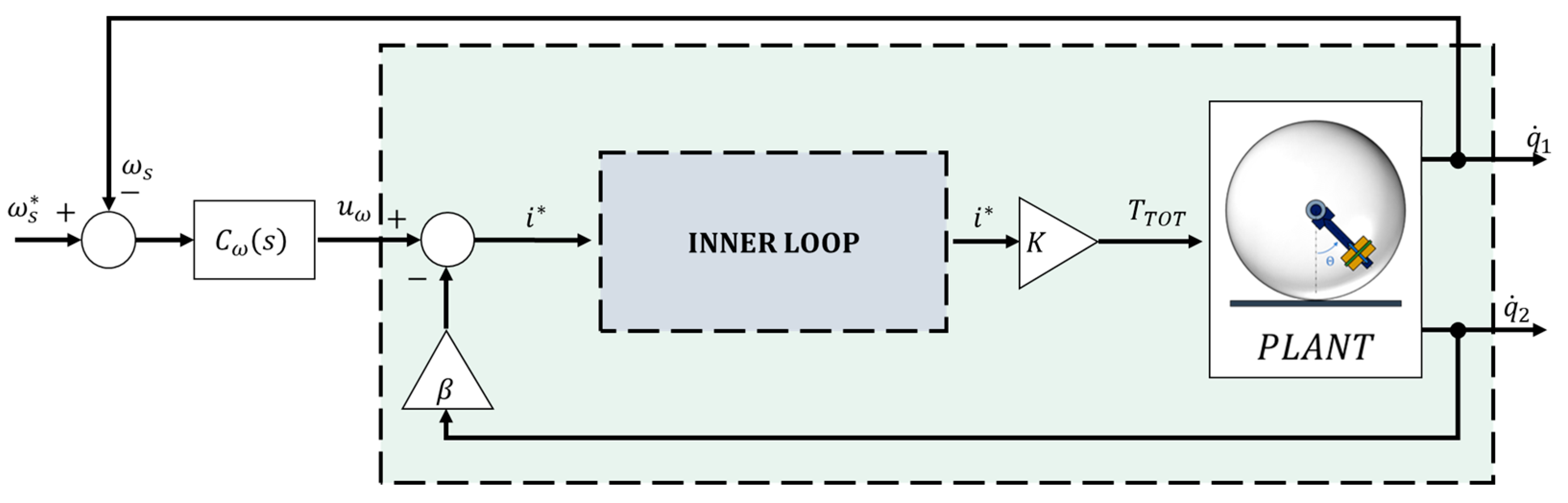
The external control loop is responsible for the SR rolling speed control. In the previous paragraph, it was explained that a proper tuning of the current controller allows to ignore the motor internal dynamics. Hence, a new block scheme is obtained (Figure 12).
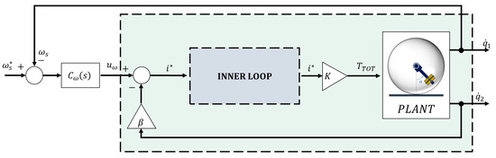
Figure 12.
Block diagram of the system ignoring the motor dynamics.
The reference armature current is calculated by subtracting the pendulum angular velocity multiplied by a constant term β to the output of the speed controller . In the next paragraphs, first, this negative feedback is studied, then the Speed Controller block is described.
5.2.1. The Viscous Friction Problem
The analytical system that has been developed includes the effects of the viscous friction of the pendulum joint and the sphere. The viscous friction is always present in real applications and contributes to the damping of the system. However, it is very difficult to determine the real values of the viscous coefficients β1 and β2. At the same time, the absence of a damping term causes the model to be unstable. The problem has been solved by including the damping effect in the control input, where the pendulum angular speed is multiplied by a constant term β and subtracted to the speed control output. This solution allowed to stabilize the system regardless of the presence of the viscous friction in the plant model. Referring to Figure 12, the input to the plant is equal to:
It can be observed that through this input, a damping effect like the one caused by the viscous friction has been introduced.
Having defined as the transfer function describing the linearization of the system inside the dark green square of Figure 12, the influence of β on its closed loop poles was studied. In particular, the closed-loop system becomes stable for values of β greater than 0.32.
5.2.2. The Speed Controller
The speed controller is designed to track a step angular velocity reference input with a value that can vary from 0 rad/s to 10 rad/s (equivalent to a linear speed of 2.5 m/s) within a maximum percentage overshoot value of 10% and a minimum settling time of 2 s. This value has been chosen based on the minimum acceleration requirement. Moreover, the controller has been designed to work when the sphere is rolling on an inclined plane with an angle of steepness that can vary from −15° to 15°.
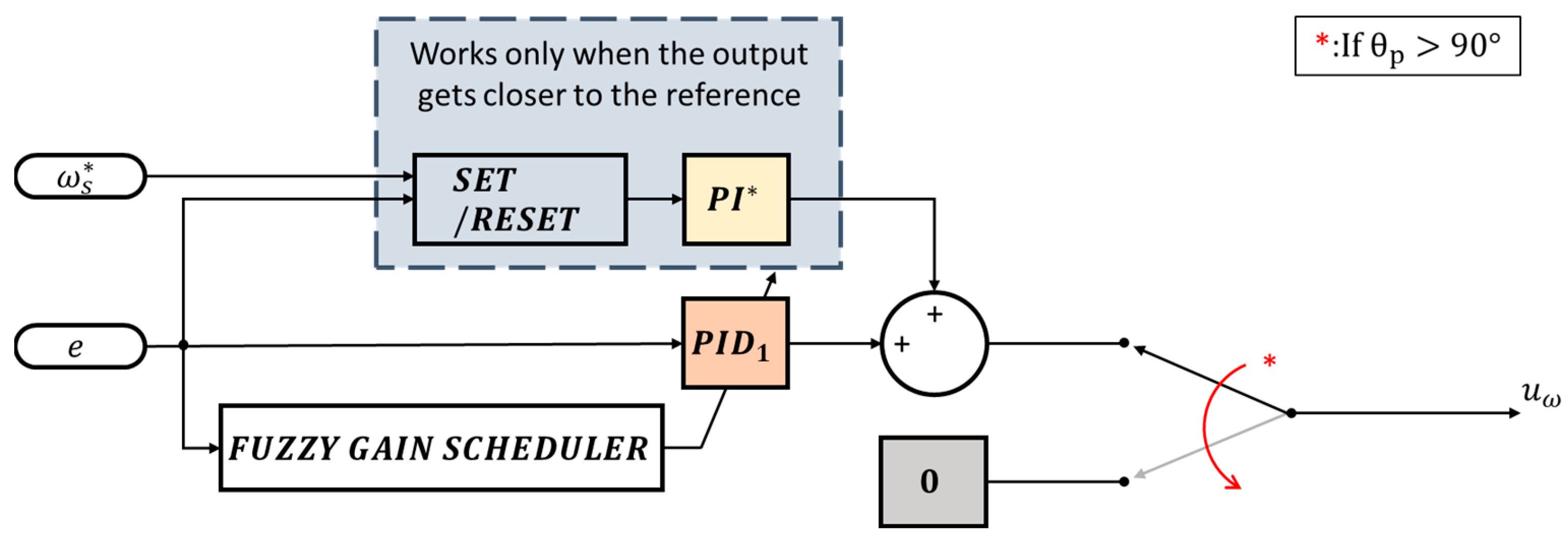
The SR is a highly non-linear system, and for this reason, a nonlinear controller is adopted. A scheme of the overall speed controller is shown in Figure 13. It can be observed that PID (Proportional Integral Derivative) and PI (Proportional Integral) controllers are used. The first one (PID1) relies on a fuzzy gain scheduler logic to perform an on-line tuning of the PID gains based on the error signal. The second one (P) is characterized by constant gains and it works only when the output gets closer to the reference input. Its objective consists of ensuring a faster convergence to the desired value, limiting the response overshoot. A set/reset block is responsible for turning on or off the P block, depending on how close the system response is to the reference input.
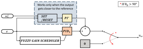
Figure 13.
Scheme of the speed controller.
Finally, a switch is used to turn to zero the output of the speed controller when the angle of the pendulum overcomes 90°. This simple solution was adopted to limit the range of motion of the pendulum without slowing down the system response.
The fuzzy gain scheduler has the following characteristics:
- The input is the error between the desired and actual angular velocity; the outputs are the three PID gains. Both the input and the output variables are identified through “Linguistic Variables”: “error” was used to refer to the input signal, and “P-gain”, “I-gain” and “D-gain” to the output ones.
- The linguistic values associated with the error are “Ze”, “S”, “M”, “L” and “XL”.
- The ones associated with the outputs are:
- P-gain: “XS”, “S”, “M”, “L” and “XL”;
- I-gain: “S” and “M”;
- D-gain: “S” and “M”.
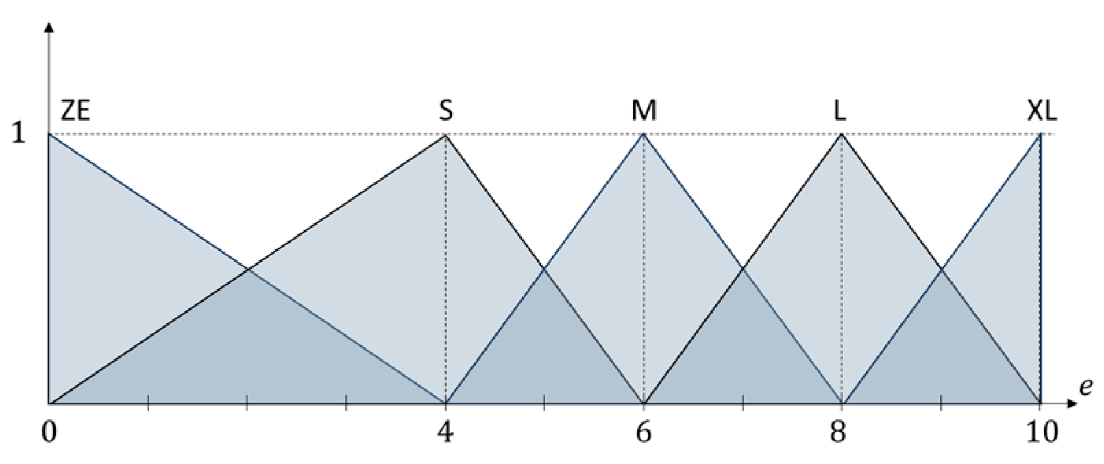
- The membership functions associated with the error and the outputs are depicted in Figure 14 and Figure 15, respectively.
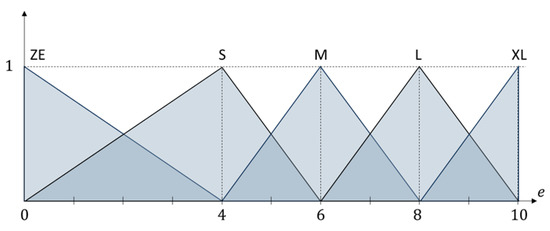 Figure 14. Error membership function.
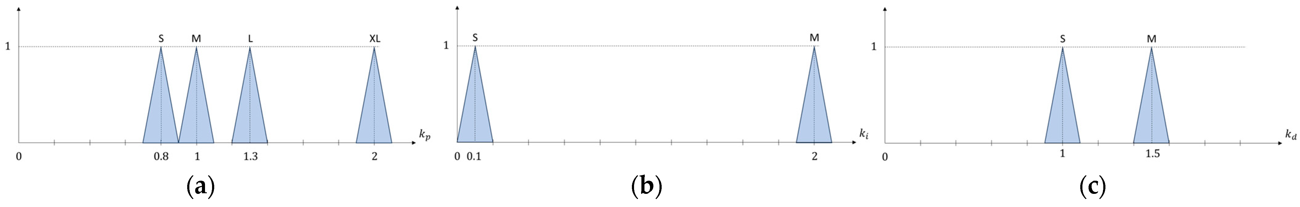
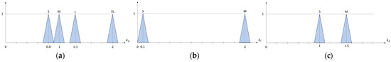 Figure 15. PID gains membership functions: (a) kp membership function; (b) ki membership function; (c) kd membership function.
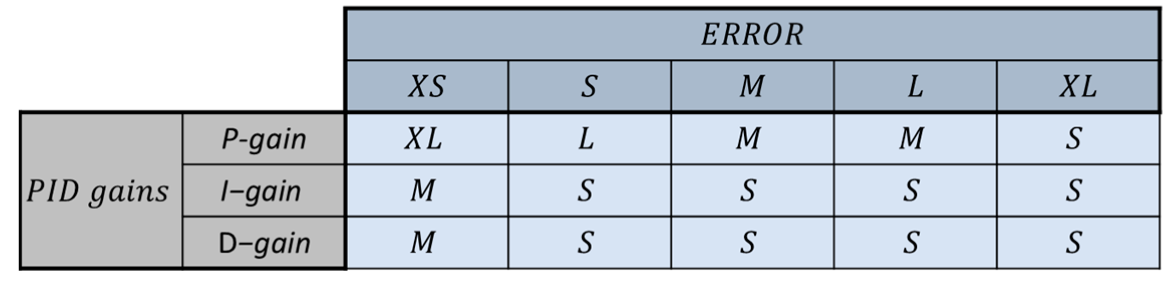
 - The rules of the fuzzy gain scheduler are depicted in Figure 16. The “centroid defuzzification method” was adopted.
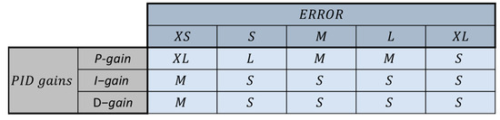 Figure 16. Fuzzy gain scheduler rules.
The P controller gains have been chosen with the objective of providing a faster convergence of the output to the reference value. Consequently, higher gains were selected with respect to the ones of the PID1, namely, kp = 4, and ki = 10. As already mentioned, to control the activation of the P controller, a set/reset block has been incorporated before it. This block enables the controller to operate only when the error is close to zero. Specifically, if the speed reference is greater than 4 rad/s, the controller starts working when the error is less than the 8% of the speed reference, while it is deactivated if it overcomes the 20%. For speed references below 4 rad/s, the percentage error is calculated relative to this velocity. The use of different threshold values (8% and 20%) for activating and deactivating the controller avoids chattering issues.
6. Results
6.1. Simulation Environment
The results reported in this section are obtained by simulating the robot motion in Simulink and Simscape multibody. In particular, two types of models are built. The first one is the analytical model, which is used for tuning the control scheme in Simulink, for a more efficient computation. The second one is the robot multibody, which is made in Simscape by importing the CAD of the components designed in Solidworks. In both, the motors are modelled as resistor-inductor circuits, where electrical parameters were given by Maxon datasheets. The motors receive input signals by the control scheme in Simulink, according to the control strategy, and the resulting driving torque is transferred to the analytical model or to the multibody joints, depending on the type of simulation. Flexible parts, where useful, are modeled according to the method defined in [38].
As regarding the multibody, to simulate the interaction between the floor and the spherical shell of the robot, the Simscape built-in block responsible for computing the spatial contact forces has been used. In particular, the normal force is modelled with stiffness and damping parameters equal to and , respectively; these values are the one suggested by the library [39] as initial guesses, and they produced good results, i.e., the robot does not vibrate in contact with the ground. The friction force is based on the Stick–slip continuous model, with a coefficient of static friction of 0.8 and a coefficient of kinetic friction of 0.4. In this case, since it is planned to cover the ball with a rubber sleeve, indicative values have been taken in the range of friction coefficients between rubber and different materials [40].
The step obstacle is modelled by introducing a solid object on the top of the floor and establishing a connection between it and the sphere, using a new spatial contact force block. This approach enables the simulation to accurately replicate the interaction between the sphere and the step, allowing for a realistic representation of the scenario.
6.2. Analysis of the Performance of the Control Strategy
In the following paragraphs, the results of the application of the linear speed controllers on the simulated SR models are presented. First, the results obtained from the analytical simulations when using the linear speed controller with the fuzzy gain scheduler are illustrated. Subsequently, the performance of this controller on the multibody model of the SR with Solidworks-designed components is showcased.
6.2.1. Test with the Analytical Model
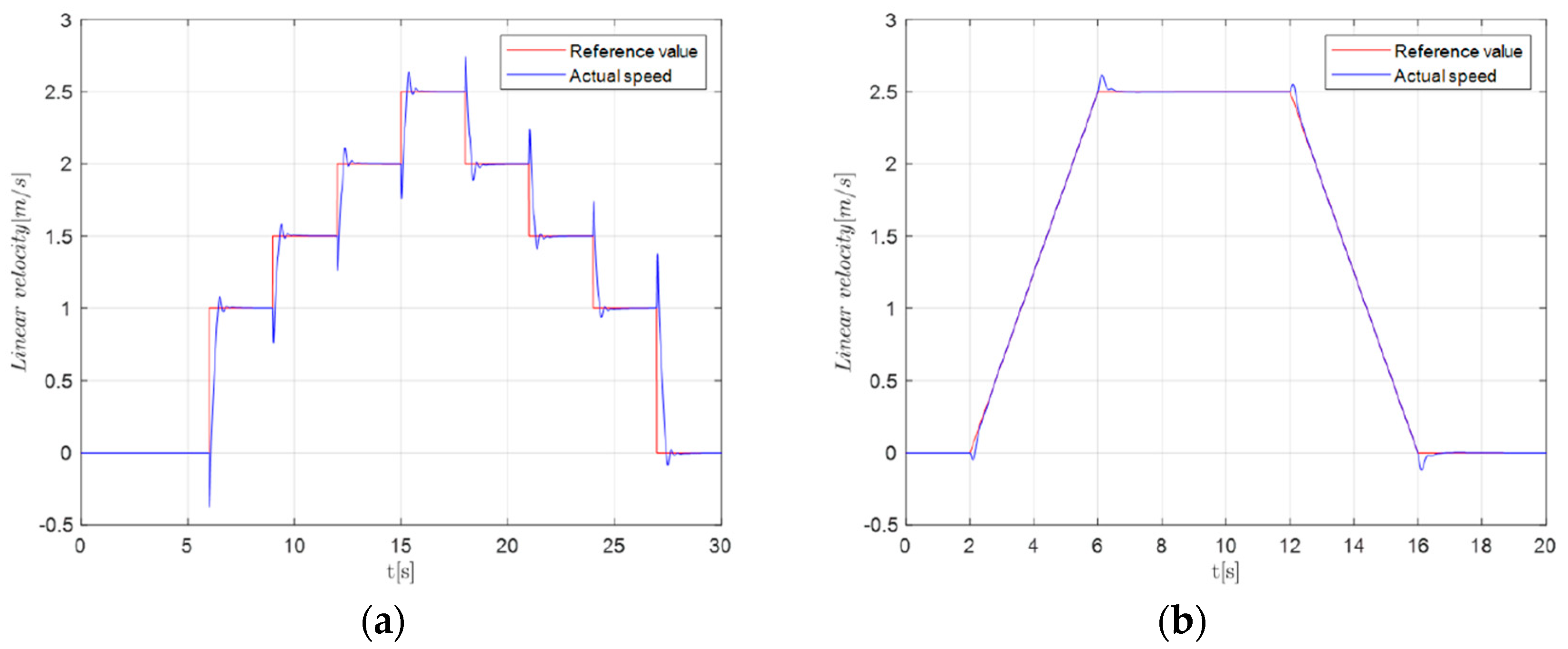
To test the control architecture and verify its functioning, two linear speed profiles have been provided as inputs for the controllers and the system response has been evaluated by comparing them with the desired one. The functioning of the system was evaluated by giving two types of input: a signal composed by subsequent velocity steps of 1 m/s, 1.5 m/s, 2 m/s and 2.5 m/s, and a trapezoidal velocity profile that reaches 2.5 m/s. The results of the analytical model of the robot with the linear speed controller are shown in Figure 17. As can be seen, the controller is able to accurately track the velocity set profile.
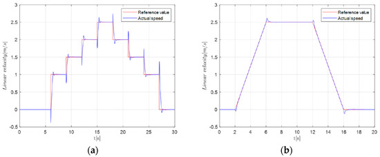
Figure 17.
Linear speed of the analytical robot model vs input speed profile. (a) Step; (b) trapezoidal profile.
6.2.2. Test with the Multibody Model
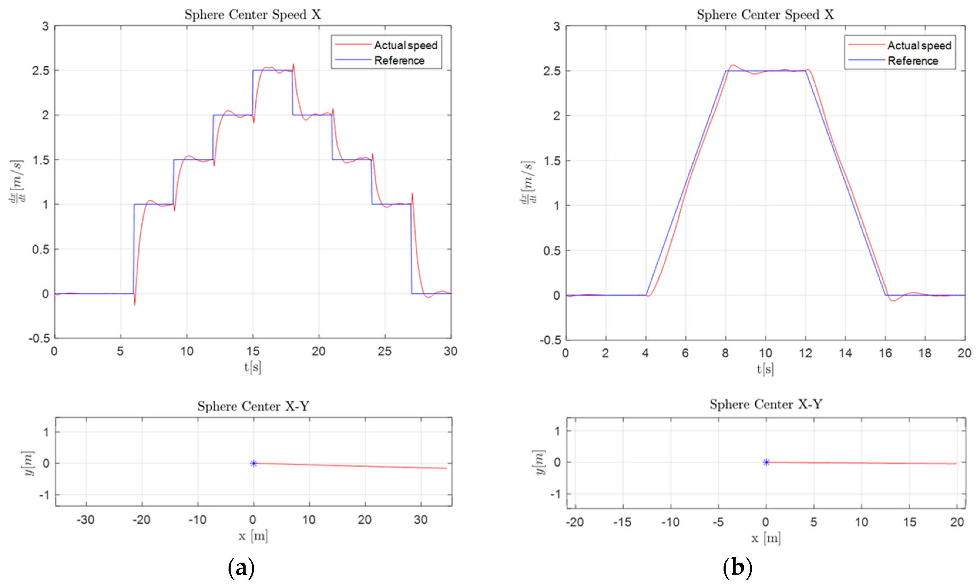
The results from testing the control architecture when the robot moves on a horizontal plane are shown in Figure 18. Similar input speed profiles that were given to the analytical model of the SR were used.
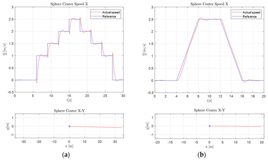
Figure 18.
Actual velocity of the simulated sphere versus velocity set. (a) Step; (b) trapezoidal.
It can be noted that the response is not as accurate as that of the analytical model, but both the velocity profiles are still well tracked by the SR. Under the sphere center speed graphs, the path followed by the robot in the XY plane during the maneuvers can be observed. It can be noted that, in the first scenario, there is a slight deviation in the negative direction of the y-axis. However, this deviation accounts for less than 0.5% of the length of the displacement along the x-axis. In the “Supplementary Materials”, the reader can find an example of simulation of a straight trajectory obtained with the presented control strategy.
6.3. Analysis of the Performance of the CMG for Step Overcoming
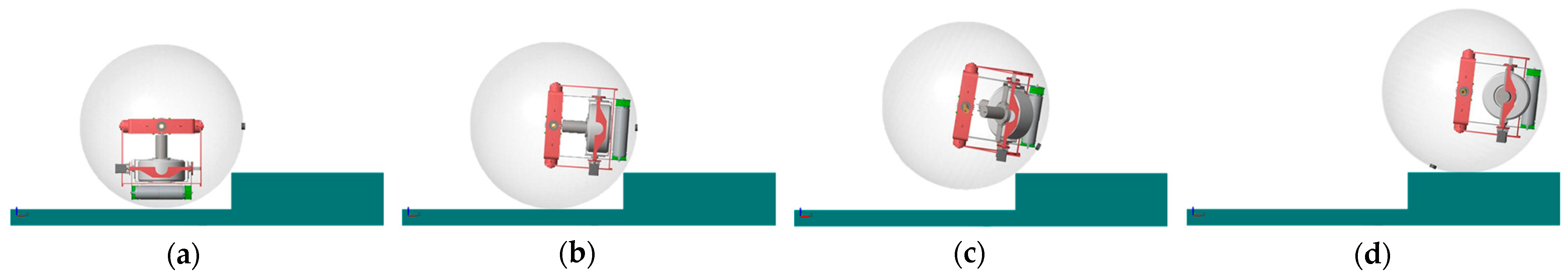
The aim of this test is to assess the capability of the robot to overcome a 100 mm step, as required. The simulations were started with the robot standstill in front of the step and the flywheel spinning at the velocity of 8000 rpm (Figure 19a). First, a torque ramp up to was provided to each pendulum motor; this permits to raise the pendulum in the horizontal position, as depicted in Figure 19b. It is remarked that, in this configuration, the mere barycenter offset does not allow the robot to overcome the obstacle. Thus, by keeping the pendulum in the horizontal configuration, the CMG system was activated with a tilting velocity of . The activation of CMG causes an initial torque increase of on the pendulum. Simultaneously, the same torque increase was provided to the pendulum motors to react to the gyroscope action. The driving torque is then the sum of pendulum and CMG effects and the shell can climb the step (Figure 19c). Notice that, during the tilting motion of the CMG, the torque increase becomes zero, following a sinusoidal law. In the simulation, the pendulum motors counteract CMG with the same torque profile and return to when the CMG effect runs out; for this, the pendulum maintains about the horizontal direction during motion (Figure 19d). For a comprehensive overview of the simulation outcome, the reader is referred to the video in the “Supplementary Materials”.
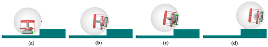
Figure 19.
Four frames of the simulation of the robot overcoming a step of 100 mm.
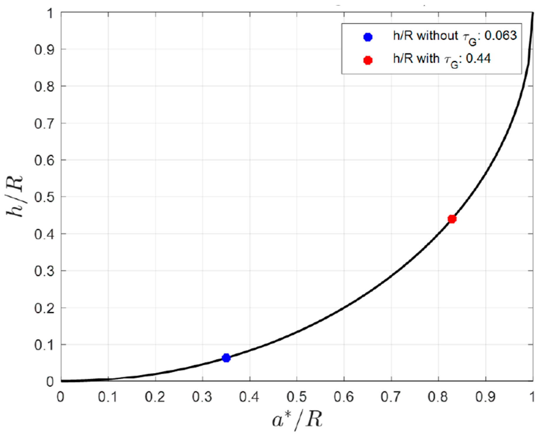
In Figure 20, the MSH-over-radius curve is plotted and two points have been marked. The blue one corresponds to the MSH over radius of this robot without the aid of the gyroscopes, which only depends on the barycenter position. The red one, instead, represents the MSH that can be theoretically overcome when the gyroscopes are functioning with the spinning and tilting velocities from Table 5. The theoretical MSH/R is increased from a value of 0.06325 to one of 0.8285, which correspond to steps of a height equal to 15.8 mm and 110 mm, respectively. Notice that, in practice, the robot is able to overcome steps < 110 mm. In fact, the theoretical value is an equilibrium point. It was for this reason that the design phase was carried out considering a MSH of 110 mm, so to satisfy the requirement of 100 mm.
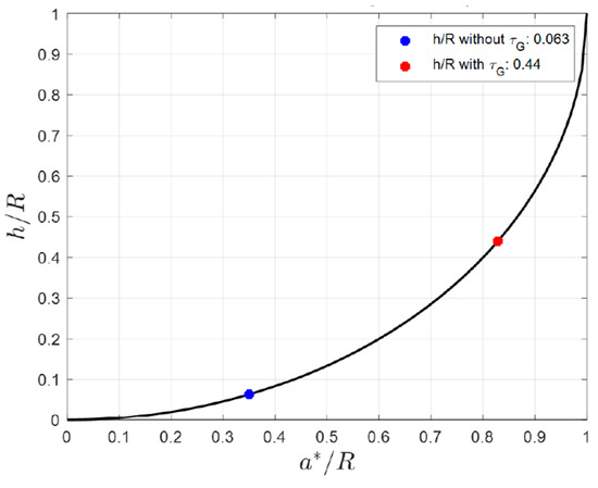
Figure 20.
MSH-over-radius curve of the spherical robot.
7. Conclusions
This research concentrates on refining a pendulum-driven spherical robot (SR), inspired by prior work by [1]. The primary aim of this study was to develop a practical solution that could improve the robot’s obstacle-climbing capability. Specifically, it focuses on improving a performance parameter called MSH (Maximum Step Height) from 25 mm to 100 mm. For a basic pendulum-driven spherical robot, it was shown that the only solution to improve the MSH value consisted in increasing the distance between the barycenter and the center of the sphere. However, this greatly complicates the design process. Alternatively, this study proposes integrating a Control Moment Gyroscope (CMG) auxiliary propulsion system. This allows for a temporary boost in maximum torque without significant displacement of the robot’s barycenter, leading to substantial MSH improvements.
The initial phase focused on studying CMG systems’ principles. A spherical robot driving mechanism using pendulum and gyroscopes was proposed. The scissored pair CMGs is introduced as an auxiliary propulsion system, coupled with the pendulum system using a differential mechanism from [1].
Following the preliminary study, the CMG design process was presented, detailing solutions to meet project requirements. Drag forces on high-speed spinning flywheels were briefly analyzed to select appropriate motors. After finalizing the CMG group design, the main motors controlling the pendulum were dimensioned to achieve a nominal robot speed of . Subsequently, the battery pack was sized to ensure a minimum 1-h runtime under the nominal operating conditions. The resulting design was a spherical UGV with a diameter and a total mass of . While batteries and hardware were not included, the dimensioning process accounted for a total mass of , allowing for the inclusion of hardware components weighing up to 4 kg while still meeting project requirements.
Simulated models of the SR were created to assess its performance. An analytical model describing straight motion was developed, and linear speed controllers were designed based on this model. More detailed multibody models of the SR were used to verify project requirements and test the designed controllers. The results showed that the CMG system effectively enhanced the robot’s obstacle-overcoming capability. The main advantage is shown in terms of the maximum height of a step obstacle, which increases to 44% of the sphere radius. This result is obtained without affecting the total mass of the robot, as the gyroscopes and their actuating systems and mechanisms are included in the mass of the pendulum.
On the other hand, it must be pointed out that the use of gyroscopes has a strong impact on the energetic balance of the robots: each single jumping maneuver requires a total amount of energy equal to 7.4% of the total battery capacity, which, if gyroscopes are not used, can ensure 72 min, or 10.8 km, running on 15° slope at 2.5 m/s. This involves that, as in any rover, a careful planning of the mission is required. For example, once the area to be explored is known, the possibility of having recharging stations at predetermined locations, the distance of which can vary according to the unevenness of the terrain, is not ruled out. In this way, the robot could move autonomously within the radius of the stations. In any case, the jump must be considered a residual option, and when possible, the selection of a new path that avoids the need for it should be preferred.
This research has significantly advanced the design of a pendulum-driven SR, providing a practical solution to enhance its obstacle-climbing ability. The integration of a CMG auxiliary propulsion system showed promise in boosting performance, but we do not rule out the possibility of expanding the CMG with an additional gimbal in order to improve the robot’s steering capabilities in the lateral direction, or to improve the robot’s stability.
There are aspects that can be explored further. For example, it will be necessary to analyze the behavior of the control strategy with different uneven terrains, or in the face of disturbances such as accidental impacts. This will make it possible to consolidate the control and evaluate its robustness. In this context, the usage of gyroscopes to improve steering capabilities can be investigated; for instance, they could be activated individually or with different tilting velocities to apply lateral torques and, at the same time, produce a boost in the direction of motion. These studies will be addressed in future works, in addition to the experimental validation of the physical prototype and the design of the control scheme for navigating curvilinear paths, as well as for dealing with inclines.
Supplementary Materials
The following supporting information can be downloaded at: https://www.mdpi.com/article/10.3390/robotics13060087/s1, Video of simulations of speed tracking control and step obstacle.
Author Contributions
Conceptualization, S.M. and M.M.; methodology, S.M. and M.M.; system design, M.M. and T.C.; modeling M.M., T.C., L.S. and M.T.; simulations: T.C., L.S., M.F. and M.T.; writing—original draft preparation, M.M., T.C. and M.F.; writing—review and editing, M.M. and M.F.; visualization, M.M. and T.C.; supervision, S.M.; project administration, S.M. funding acquisition, S.M. All authors have read and agreed to the published version of the manuscript.
Funding
This research received no external funding.
Data Availability Statement
Data is contained within the article or Supplementary Material.
Conflicts of Interest
The authors declare no conflicts of interest.
References
- Melchiorre, M.; Salamina, L.; Mauro, S.; Pastorelli, S. Design of a Spherical UGV for Space Exploration. Int. Astronaut. Congr. 2022, 2022, 18–22. [Google Scholar]
- Chase, R.; Pandya, A. A review of active mechanical driving principles of spherical robots. Robotics 2012, 1, 3–23. [Google Scholar] [CrossRef]
- Bujňák, M.; Pirník, R.; Rástočný, K.; Janota, A.; Nemec, D.; Kuchár, P.; Tichý, T.; Łukasik, Z. Spherical Robots for Special Purposes: A Review on Current Possibilities. Sensors 2022, 22, 1413. [Google Scholar] [CrossRef] [PubMed]
- Kaznov, V.; Seeman, M. Outdoor navigation with a spherical amphibious robot. In Proceedings of the IEEE/RSJ 2010 International Conference on Intelligent Robots and Systems (IROS), Taipei, Taiwan, 18–22 October 2010; pp. 5113–5118. [Google Scholar] [CrossRef]
- Seeman, M.; Broxvall, M.; Saffiotti, A.; Wide, P. An Autonomous Spherical Robot for Security Tasks. In Proceedings of the CIHSPS 2006—IEEE International Conference on Computational Intelligence for Homeland Security and Personal Safety, Alexandria, VA, USA, 16–17 October 2006; pp. 51–55. [Google Scholar] [CrossRef]
- Yang, M.; Tao, T.; Huo, J.; Neusypin, K.A.; Zhang, Z.; Zhang, H.; Guo, M. Design and Analysis of a Spherical Robot with Two Degrees of Freedom Swing. In Proceedings of the 32nd Chinese Control and Decision Conference (CCDC), Hefei, China, 22–24 August 2020; pp. 4913–4918. [Google Scholar] [CrossRef]
- Rossi, A.P.; Maurelli, F.; Unnithan, V.; Dreger, H.; Mathewos, K.; Pradhan, N.; Corbeanu, D.-A.; Pozzobon, R.; Massironi, M.; Ferrari, S.; et al. Daedalus—Descent and Exploration in Deep Autonomy of Lava Underground Structures; University of Würzburg: Würzburg, Germany, 2021. [Google Scholar] [CrossRef]
- Ye, P.; Sun, H.; Qiu, Z.; Chen, J. Design and Motion Control of a Spherical Robot with Stereovision. In Proceedings of the 2016 IEEE 11th Conference on Industrial Electronics and Applications (ICIEA), Hefei, China, 5–7 June 2016; pp. 1267–1282. [Google Scholar] [CrossRef]
- Wang, F.; Li, C.; Niu, S.; Wang, P.; Wu, H.; Li, B. Design and Analysis of a Spherical Robot with Rolling and Jumping Modes for Deep Space Exploration. Machines 2022, 10, 126. [Google Scholar] [CrossRef]
- Zhao, B.; Li, M.; Yu, H.; Sun, L. Dynamics and motion control of a two pendulums driven spherical robot. In Proceedings of the IEEE/RSJ 2010 International Conference on Intelligent Robots and Systems, Taipei, Taiwan, 18–22 October 2010; pp. 147–153. [Google Scholar] [CrossRef]
- Yoon, J.-C.; Ahn, S.-S.; Lee, Y.-J. Spherical Robot with New Type of Two-Pendulum Driving Mechanism. In Proceedings of the 15th International Conference on Intelligent Engineering Systems, Poprad, Slovakia, 23–25 June 2011; pp. 275–279. [Google Scholar]
- Karavaev, Y.L.; Kilin, A.A. The dynamics and control of a spherical robot with an internal omniwheel platform. Regul. Chaotic Dyn. 2015, 20, 134–152. [Google Scholar] [CrossRef]
- Ba, P.D.; Hoang, Q.D.; Lee, S.-G.; Nguyen, T.H.; Duong, X.Q.; Tham, B.C. Kinematic Modeling of Spherical Rolling Robots with a Three-Omnidirectional-Wheel Drive Mechanism. In Proceedings of the 20th International Conference on Control, Automation and Systems (ICCAS), Busan, Korea, 13–16 October 2020; pp. 463–466. [Google Scholar] [CrossRef]
- Liu, W.; Sun, J.; Wang, R.; Geng, G.; Han, X. Heavy-duty spherical mobile robot driven by five omni wheels. Proc. Int. Conf. Artif. Life Robot. 2020, 25, 720–723. [Google Scholar] [CrossRef]
- Zhan, Q.; Cai, Y.; Yan, C. Design, Analysis and Experiments of an Omni-directional Spherical Robot. In Proceedings of the IEEE International Conference on Robotics and Automation, Shanghai, China, 9–13 May 2011; pp. 4921–4926. [Google Scholar]
- Singh, A.; Paigwar, A.; Manchukanti, S.T.; Saroya, M.; Chiddarwar, S. Design and motion analysis of Compliant Omni- directional Spherical Modular Snake Robot (COSMOS). In Proceedings of the International Conference on Reconfigurable Mechanisms and Robots (ReMAR), Delft, The Netherlands, 20–22 June 2018. [Google Scholar] [CrossRef]
- Sang, S.; Zhao, J.; Wu, H.; Chen, S.; An, Q. Modeling and simulation of a spherical mobile robot. Comput. Sci. Inf. Syst. 2010, 7, 51–62. [Google Scholar] [CrossRef]
- Tafrishi, S.A.; Svinin, M.; Esmaeilzadeh, E.; Yamamoto, M. Design, modeling, and motion analysis of a novel fluid actuated spherical rolling robot. J. Mech. Robot. 2019, 11, 041010. [Google Scholar] [CrossRef]
- Ho, K.Y.; Mayer, N.M. Implementation of a mobile spherical robot with shape-changed inflatable structures. In Proceedings of the International Conference on Advanced Robotics and Intelligent Systems (ARIS), Taipei, Taiwan, 6–8 September 2017; pp. 104–109. [Google Scholar] [CrossRef]
- Artusi, M.; Potz, M.; Aristiźabal, J.; Menon, C.; Cocuzza, S.; Debei, S. Electroactive elastomeric actuators for the implementation of a deformable spherical rover. IEEE/ASME Trans. Mechatron. 2011, 16, 50–57. [Google Scholar] [CrossRef]
- Kamon, S.; Bunathuek, N.; Laksanacharoen, P. A three-legged reconfigurable spherical robot No.3. In Proceedings of the 2021 30th IEEE International Conference on Robot and Human Interactive Communication (RO-MAN), Vancouver, BC, Canada, 8–12 August 2021; Institute of Electrical and Electronics Engineers Inc.: Piscataway, NJ, USA, 2021; pp. 426–433. [Google Scholar] [CrossRef]
- Aoki, T.; Asami, K.; Ito, S.; Waki, S. Development of quadruped walking robot with spherical shell: Improvement of climbing over a step. Robomech J. 2020, 7, 22. [Google Scholar] [CrossRef]
- Zhang, M.; Chai, B.; Cheng, L.; Sun, Z.; Yao, G.; Zhou, L. Multi-movement spherical robot design and implementation. In Proceedings of the 2018 IEEE International Conference on Mechatronics and Automation (ICMA), Changchun, China, 5–8 August 2018; pp. 1464–1468. [Google Scholar] [CrossRef]
- Schroll, G.C. Design of a Spherical Vehicle with Flywheel Momentum Storage for High Torque Capabilities; Massachusetts Institute of Technology: Cambridge, MA, USA, 2008. [Google Scholar]
- Bilous, V.; Andulkar, M.; Berger, U. Design of a novel spherical robot with high dynamic range and maneuverability for flexible applications. In Proceedings of the 50th International Symposium on Robotics (ISR), Munich, Germany, 20–21 June 2018; pp. 64–69. [Google Scholar]
- Chen, J.; Ye, P.; Sun, H.; Jia, Q. Design and Motion Control of a Spherical Robot with Control Moment Gyroscope. In Proceedings of the 3rd International Conference on Systems and Informatics (ICSAI), Shanghai, China, 19–21 November 2016. [Google Scholar]
- Kim, H.W.; Jung, S. Design and Control of a Sphere Robot Actuated by a Control Moment Gyroscope. In Proceedings of the 19th International Conference on Control, Automation and Systems (ICCAS), Jeju, Korea, 15–18 October 2019; pp. 1287–1290. [Google Scholar] [CrossRef]
- Li, C.; Zhu, A.; Zheng, C.; Mao, H.; Arif, M.A.; Song, J.; Zhang, Y. Design and analysis of a spherical robot based on reaction wheel stabilization. In Proceedings of the 2022 19th International Conference on Ubiquitous Robots (UR), Jeju, Republic of Korea, 4–6 July 2022; Institute of Electrical and Electronics Engineers Inc.: Piscataway, NJ, USA, 2022; pp. 143–148. [Google Scholar] [CrossRef]
- Dudley, C.J.; Woods, A.C.; Leang, K.K. A micro spherical rolling and flying robot. In Proceedings of the IEEE International Conference on Intelligent Robots and Systems (IROS), Hamburg, Germany, 28 September–2 October 2015; pp. 5863–5869. [Google Scholar] [CrossRef]
- Sabet, S.; Agha-Mohammadi, A.A.; Tagliabue, A.; Elliott, D.S.; Nikravesh, P.E. Rollocopter: An Energy-Aware Hybrid Aerial-Ground Mobility for Extreme Terrains. In Proceedings of the 2019 IEEE Aerospace Conference, Big Sky, MT, USA, 2–9 March 2019. [Google Scholar] [CrossRef]
- Shi, L.; Hu, Y.; Su, S.; Guo, S.; Xing, H.; Hou, X.; Liu, Y.; Chen, Z.; Li, Z.; Xia, D. A Fuzzy PID Algorithm for a Novel Miniature Spherical Robots with Three-dimensional Underwater Motion Control. J. Bionic Eng. 2020, 17, 959–969. [Google Scholar] [CrossRef]
- Gu, S.; Guo, S.; Zheng, L. A highly stable and efficient spherical underwater robot with hybrid propulsion devices. Auton. Robot. 2020, 44, 759–771. [Google Scholar] [CrossRef]
- Li, T.; Liu, W. Design and Analysis of a Wind-Driven Spherical Robot with Multiple Shapes for Environment Exploration. J. Aerosp. Eng. 2011, 24, 135–139. [Google Scholar] [CrossRef]
- Antol, J.; Calhoum, P.C.; Flick, J.J.; Hajos, G.; Key, J.P.; Stillwagen, F.H.; Krizan, S.A.; Strickland, C.V.; Owens, R.; Wisniewski, M. Low Cost Mars Surface Exploration: The Mars Tumbleweed; NTRS: Hampton, Virginia, 2003. Available online: http://www.sti.nasa.gov (accessed on 17 April 2024).
- Xie, S.; Chen, J.; Luo, J.; Yao, H.L.J.; Gu, J. Dynamic Analysis and Control System of Spherical Robot for Polar Region Scientific Research. In Proceeding of the 2013 IEEE International Conference on Robotics and Biomimetics (ROBIO), Shenzhen, China, 12–14 December 2013; pp. 2540–2545. [Google Scholar] [CrossRef]
- Ylikorpi, T.; Suomela, J. Ball-shaped Robots. In Climbing and Walking Robots: Towards New Applications; Zhang, H., Ed.; InTech: Revesby, NSW, Australia, 2007; pp. 235–256. [Google Scholar]
- Genta, G. Kinetic Energy Storage: Theory and Practice of Advanced Flywheel Systems; Butterworths: Boston, MA, USA, 1985. [Google Scholar]
- Salamina, L.; Botto, D.; Mauro, S.; Pastorelli, S. Modeling of flexible bodies for the study of control in the Simulink environment. Appl. Sci. 2020, 10, 5861. [Google Scholar] [CrossRef]
- Mathworks Modeling Contact Force between Two Solids. Available online: https://it.mathworks.com/help/sm/ug/modeling-contact-force-between-two-solids.html (accessed on 17 May 2024).
- Engineers Edge Coefficient of Friction Equation and Table Chart. Engineers Edge. Available online: https://www.engineersedge.com/coeffients_of_friction.htm (accessed on 18 May 2024).


Disclaimer/Publisher’s Note: The statements, opinions and data contained in all publications are solely those of the individual author(s) and contributor(s) and not of MDPI and/or the editor(s). MDPI and/or the editor(s) disclaim responsibility for any injury to people or property resulting from any ideas, methods, instructions or products referred to in the content. |
© 2024 by the authors. Licensee MDPI, Basel, Switzerland. This article is an open access article distributed under the terms and conditions of the Creative Commons Attribution (CC BY) license (https://creativecommons.org/licenses/by/4.0/).