Abstract
We describe a quantum teleportation protocol for exchanging data between a mobile robot and its control station. Because of the high cost of quantum network systems, we use MATLAB software to simulate the teleportation of data. Our simulation models the dynamic motion of a car-like mobile robot (CLMR), considering its mass and inertia and the environmental viscosity. Our remote control method accurately reproduces a mathematical model of the CLMR’s real-world motion. The CLMR’s trajectory is represented by differential equations, with the velocity calculated using the Jacobian matrix. The velocity inputs are teleported from the control station to the CLMR, enabling it to move. Nevertheless, physical constraints cause the deviation of the robot’s trajectory from the predicted trajectory. To correct this deviation, the CLMR’s current position is teleported to the control station. Before implementing this protocol, we calculate the quantum teleportation circuit, and we use quantum gates in matrix form to simulate the data teleportation process. The protocol’s accuracy is assessed by comparing the original data and teleported data, and a good match is obtained. This study demonstrates the feasibility of quantum teleportation for remotely controlling real-time robotic systems over long distances and in environments that interfere with classical wireless communication.
1. Introduction
In recent years, quantum computing techniques have transformed various industries. In robotics, they have improved several aspects of robotic systems, such as path planning and simultaneous localization and mapping. Petschnigg et al. [1] identified prospective application areas and open research subjects of quantum computing, such as the application of quantum computing tools to artificial intelligence and machine learning for increased efficiency and accuracy in robotic systems. Gehlot et al. [2] developed an approach that employed quantum superposition and entanglement to solve difficult robotic differential equations. Lathrop et al. [3] developed quantum fast planning and scheduling (q-FPS) and quantum-rapid-exploring random tree (q-RRT) algorithms to enhance robot navigation performance. Quantum computing tools can also be used to reduce the total distance travelled by robots. Atchade-Adelomou et al. [4] solved the travelled distance problem of mobile robots by implementing a quantum combinatorial optimization algorithm and distributing data computation not only to the central computer but also to each robot. Koshelev et al. [5] focused on improving overall navigation by building intelligent control algorithms for mobile robots equipped with redundant manipulators and stereovision using quantum and soft computing. These technologies enable a robot to adapt to dynamic settings while improving its decision-making and navigation capabilities. Vella et al. [6] examined upgrading a robot’s path planning using a quantum technique inspired by Grover’s algorithm to translate traditional Boolean computation into a quantum framework.
The question of whether quantum computing can improve robot navigation by increasing autonomy has been addressed. Khoshnoud et al. [7] investigated this topic by combining aspects of quantum entanglement and quantum cryptography and integrating them into distributed robotic platforms to increase overall robot autonomy. Zhai and Feng [8] improved a robot’s performance by solving optimization problems through the use of search capabilities and global exploration strategies. This was achieved by developing an enhanced ant colony optimization algorithm that combined artificial potential fields and quantum evolution theory. Quantum particle swarm optimization (QPSO) algorithms are another approach to solving real-time path-planning optimization problems. Li and Wu [9] proposed a hybrid algorithm consisting of quantum-leading-following-based optimization and an obstacle avoidance strategy to improve the search capabilities of mobile robots. Dong et al. [10] observed that their particle swarm optimization technique easily fell into local optima while also incurring a large computational cost. To address this issue, they enhanced the approach to self-adjusting the weight factor and increased the convergence speed. Fernandes et al. [11] encountered the same problem of falling into local minima, which they overcame by incorporating peaks of diversity in the algorithm’s population. As a result, they were able to create safe and efficient pathways while minimizing energy loss.
Quantum computing algorithms can be used to optimize coordination and communication among robots in the same swarm. To achieve this aim, Maria et al. [12] chose an approach that involved building a robotic swarm system to improve its scalability and resilience. Chella et al. [13] worked on a similar problem but focused on establishing a quantum-based decision-making system for the path planning of a group of robots. Mechatronic systems can be merged with quantum computing to develop quantum mechatronics, a quantum technology employed to build highly efficient engineering platforms. Lamata et al. [14] focused on this problem by constructing quantum robotics and macroscopic. Wang et al. used quantum computing with better proximal policy optimization to enhance a model’s performance in path-tracking tasks [15]. During their experiment, a lack of real interaction samples was observed. To address this issue, they combined fake samples with real ones in a specific proportion.
Quantum computing is revolutionizing mobile robotics, including the fields of unmanned aerial vehicles (UAVs), unmanned surface vehicles (USVs), and autonomous underwater vehicles (AUVs). Wang et al. [16] developed a QPSO algorithm for a USV that works in real time to ensure the optimal path while avoiding obstacles. Wang et al. [17] conducted a similar experiment to solve path planning for AUVs. Their improved QPSO addressed the typical constraints of the convergence and optimization capabilities of QPSO. Liu et al. [18] chose UAVs in preference to satellites to distribute entangled quantum states over long distances. This decision was motivated by the complexity and high cost of satellites, whereas quantum communications can provide a practical full-time and all-weather alternative. Other researchers have investigated the use of quantum computing to improve drone navigation. For example, Park et al. [19] focused on the optimization of UAV decision-making processes. It is critical to note that quantum computing can cause scalability issues due to the near-intermediate-scale quantum restriction. To address this issue, a quantum centralized critic has been used. Quantum teleportation is a key technology in quantum computing that has revolutionized engineering industries. It involves transferring a particle’s quantum state to another particle located a significant distance away. This procedure does not require physical movement of the quantum state; rather, the original quantum state is destroyed at the sender’s position and restored at the receiver’s position. As a result, many scientists worldwide have included quantum teleportation in their research projects because of its promise in information processing, cryptography, and communication. Anderson et al. [20] chose quantum networks over the traditional telecommunications fiber network to reliably transport data using quantum dots, which are semiconductor nanocrystals that emit light in the telecom C-band. El Kirdi et al. [21] performed groundbreaking work in extending the applications of quantum teleportation to a broader range of physical systems by entangling the qubit of a continuous-variable system and then teleporting the qubit state into a discrete system. Another use of quantum teleportation was reported by Salimian et al. [22], who presented a quantum teleportation system for transferring the state of two superconducting qubits from one lab to another. This was realized by connecting superconducting qubits with each other and with LC resonators.
During quantum teleportation, faults may emerge in the form of arbitrary noises. To address this difficulty, Zhang et al. [23] designed a two-part scheme, comprising feed-forward control followed by a decoherence channel, that enables an entangled qubit to be transferred. They then measured the noise environment associated with the entangled qubit in the decoherence channel. Villaseñor and Malaney [24] used continuous-variable non-Gaussian states as quantum teleportation resource states to teleport coherent and compressed states via noisy channels. Bolokian et al. [25] investigated the effects of amplitude-damping noise and bit-flip noise by creating a protocol that sends two single-qubit states from Alice to Bob and a three-qubit entangled state in the other direction. Bolokian et al. [26] demonstrated the robustness of a bidirectional quantum teleportation technique that allows quantum states to be shared.
Quantum teleportation has made it feasible to control and secure dynamic systems, increasing their speed, dependability, and resistance to cyberattacks. Khoshnoud et al. [27] examined this issue and proposed a quantum-based technique for securing and improving data transmission across automated control systems. Panda et al. [28] adopted the novel strategy of remotely controlling the direction of a quantum-controlled mobile robot using Zidan’s quantum computing algorithm. Khoshnoud et al. [29] applied quantum techniques to autonomous mobile systems in two steps. The first step involved incorporating quantum entanglement and quantum cryptography in macroscopic mechanical systems, and the second involved teleporting quantum states via classical and Einstein–Podolsky–Rosen channels to improve the control of dynamical systems and the autonomy of mobile platforms. Hongtao et al. [30] proposed a safe bidirectional quantum key distribution protocol, one of the quantum teleportation methods used in the Internet of Vehicles (IoV), for information security. Although their report did not include sufficient details and tests for their method to be widely applied to IoV security requirements, the outcomes were satisfactory. Chiti et al. [31] used quantum teleportation and entanglement swapping between drones to construct entanglement-based states. These states were subsequently used for quantum computing distribution and E91, a quantum key distribution technique. Mastriani et al. [32] conducted an interesting three-step experiment. The first step was to create and distribute two entangled photons from a quantum satellite to two drones over clouds. The second step involved the drones plunging into the clouds until they reached an altitude that allowed for a strong connection with a mobile ground station, then each drone created an entangled photon pair and distributed one of them to the nearest mobile ground station. The final stage involved each drone teleporting the entangled photon that it received from the quantum satellite to the nearest mobile ground station. Ciobanu et al. [33] utilized a hybrid land–satellite network for quantum communication between satellites and a ground station. They employed a framework to distribute entangled photons to two distant nodes via a constellation of satellites able to retransmit a photon beam. Satellites can even be used as central servers [34] by developing variational quantum algorithms that train collaborative learning locally, focusing on the complexity emerging from vast datasets and machine learning models. Thus, quantum teleportation can be used to secure long-distance data transmission between high-altitude platform stations and UAVs, which route quantum information to the ground station. Gonzalez-Raya et al. [35] attempted quantum teleportation between a fixed station and a satellite in turbulent air. They focused on the degradation of entanglement due to many causes of errors in the distribution, such as atmospheric changes, turbulence, and detector inefficiency. The results revealed that their quantum teleportation procedure was inefficient under such settings. To compensate, they included an intermediary station for either state generation or beam focusing to reduce the impact of atmospheric turbulence. Mastriani et al. [36] demonstrated that quantum teleportation can be used in hybrid systems consisting of submarines and satellites by developing a quantum teleportation protocol composed of two submerged nuclear submarines located on opposite sides of an ocean and a quantum satellite that transmits entangled pairs and optical disambiguation bits to buoys located on the sea surface associated with these submerged submarines.
The reviewed studies underline the significance of establishing high-quality connections between autonomous systems. This work presents the use of teleportation in the real-time wireless control of mobile robots, proposing a wireless connection that provides velocity inputs from the control station to a car-like robot and subsequently returns the robot’s current position to the station. The strategy used is to simulate data exchange between the two platforms using a novel quantum teleportation protocol, with the goal of increasing the speed and accuracy of the data delivered.
Section 2 describes the robot’s model and quantum computing tools such as teleportation using the Bell state and entanglement. The system’s architecture is then described in detail, along with the implementation of remote control for the mobile robot. Section 3 presents and discusses the simulation results, which is followed by a conclusion with a perspective in Section 4.
2. Materials and Methods
2.1. Car-like Mobile Robot
Car-like mobile robots (CLMRs) are autonomous robotic systems designed to behave like automobiles in their wheel mobility, steering mechanism, control, and navigation. In this study, we develop a novel quantum teleportation algorithm to simulate a wireless connection between a control station and the controller of a robot. The idea is to send and receive information in parallel about its longitudinal and angular velocities and the coordinates of its position with respect to the x-, y-, and z-axes. We implement a car dynamic motion algorithm that considers parameters including the mass, inertia, length, width, and coefficient of viscous friction. The robot’s desired position and orientation input commands in three-dimensional space are given as follows:
- x(t)—Robot’s motion in x-direction;
- y(t)—Robot’s motion in y-direction;
- z(t)—Angle between robot’s direction and x-axis.
The desired velocity and acceleration of the robot in its own configuration space are, respectively, the first- and second-time derivatives of the desired positions [1]:
The kinematic and dynamic equations of the CLMR in Cartesian coordinate systems can be used to clarify its motion.
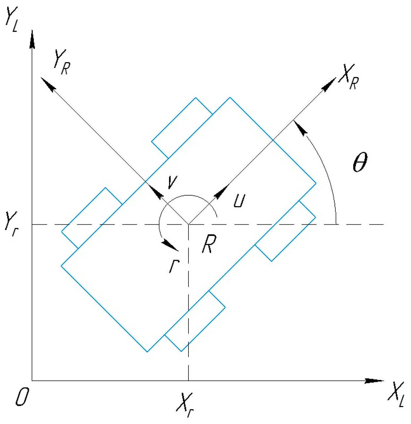
The CLMR has a configuration in the Cartesian coordinate system , whose origin is at the robot’s center of gravity. There is also a world Cartesian coordinate system , in which the motion of the CLMR can be observed (Figure 1). The robot’s instantaneous velocities u, v, and r with respect to its world frame are known. This information can be used to find the instantaneous velocities in the robot’s configuration space.
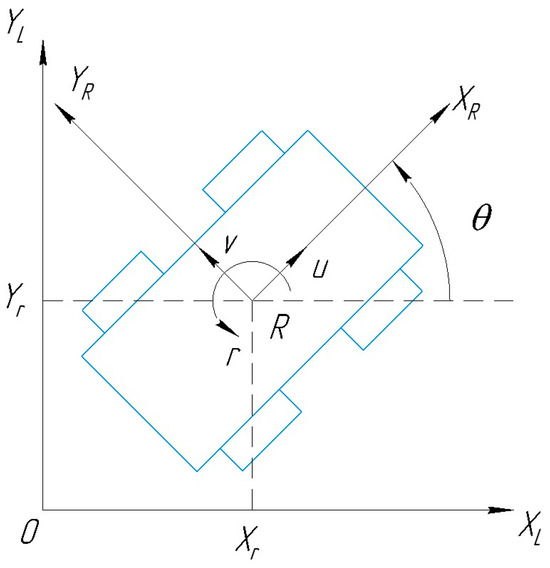
Figure 1.
Mobile robot kinematics on a two-dimensional (2D) planar surface (Image adapted from [1]).
The kinematic equations of the robot’s motion can be expressed as follows:
- —Longitudinal velocity;
- —Lateral velocity;
- —Angular velocity;
- —Angle between robot’s longitudinal state vector and global x-axis.
For ease of calculation, the kinematic equations of motion are expressed in matrix form. The inverse differential kinematic equations are as follows:
- —Velocity of CLMR;
- —Inverse of Jacobian matrix that transforms velocity vector with respect to body-fixed frame to velocity vector with respect to world frame.
The CLMR cannot move in the direction perpendicular to its vector state. This means that it can only move forward or backward; there is also a steering mechanism that allows the robot to move left and right. This mechanism is based on the steering angle , which is the angle between the directions of the front and the rear tires around the steering axis:
- —Length of CLMR;
- —Resultant of longitudinal and lateral velocities.
To mimic the mechanical constraints of the steering mechanism, the steering angle is limited to a minimum of and a maximum of , where angles with negative (positive) values indicate left (right) turns. Because the CLMR is a nonholonomic system, the lateral velocity must be zero:
- —Nonholonomic velocity of CLMR;
- —Nonholonomic longitudinal velocity;
- —Nonholonomic lateral velocity;
- —Nonholonomic angular velocity;
- —State nonholonomic matrix;
- —Resultant of longitudinal, lateral, and angular velocities with respect to fixed frame.
The first derivative of the velocity in the CLMR’s configuration space in Equation (5) gives its acceleration in this space:
By substituting the CLMR’s velocity in Equation (5), we obtain
Because the CLMR is a nonholonomic system, the lateral acceleration must be zero. The equation of its acceleration becomes
- —Nonholonomic acceleration of CLMR;
- —Nonholonomic longitudinal acceleration;
- —Nonholonomic lateral acceleration;
- —Nonholonomic angular acceleration;
- —State nonholonomic matrix;
- —Resultant of longitudinal, lateral, and angular accelerations.
The dynamic equations of motion enable the design and control of the CLMR, increasing its path-following performance. The dynamic equations are obtained using the following Euler–Lagrange equation:
- KE—Kinetic energy;
- PE—Potential energy.
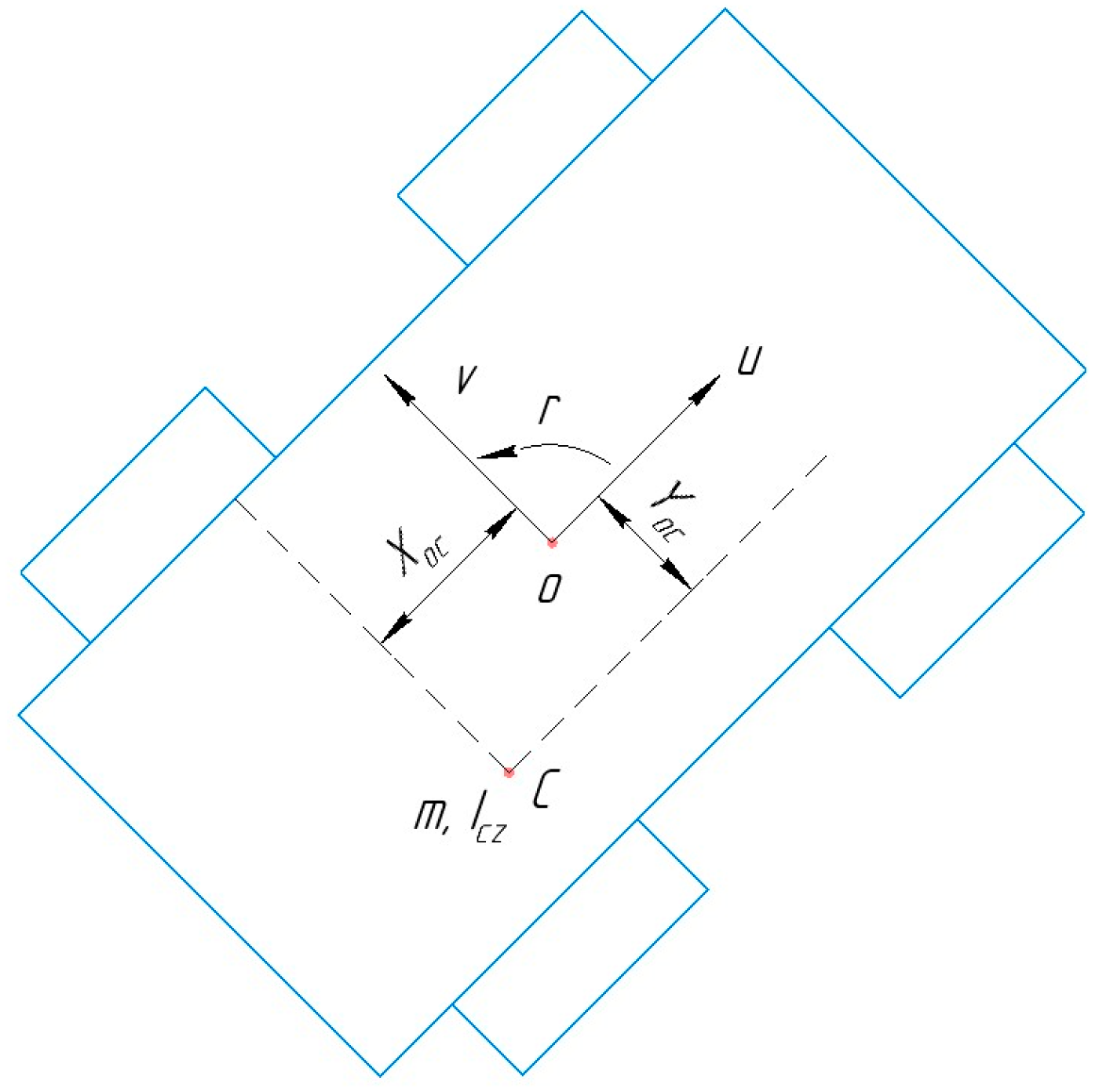
Figure 2 depicts the dynamical parameters of the robot.
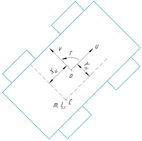
Figure 2.
Mobile robot dynamics in a 2D planar surface (Image adapted from [1]).
For a land-based robot, the potential energy is always zero. Therefore, the Lagrangian equation becomes [1]
- —Total mass of robot;
- —Velocity at center of inertia with respect to x-axis;
- —Velocity at center of inertia with respect to y-axis;
- —Moment of inertia with respect to z-axis;
- —Angular velocity with respect to z-axis.
The velocities at the center of inertia with respect to the x- and y-axes are as follows:
- —Distance between origin of body frame and center of inertia with respect to x-axis;
- —Distance between origin of body frame and center of inertia with respect to y-axis.
Substituting Equation (14) into the Lagrangian in Equation (13) gives
The Euler–Lagrange equations can be computed as
The equations of motion with respect to the fixed frame are
The origin of the body frame coincides with the center of inertia, meaning that the distance between them with respect to the x- and y-axes is zero ( and ).
The longitudinal force and moment of inertia applied to the CLMR influence its displacement. The dynamic equations of the CLMR’s motion can then be expressed in matrix form as follows:
- —Nonholonomic acceleration of CLMR;
- —Torque vector of CLMR;
- —Dynamic matrix of CLMR;
- —Other effects of CLMR.
From the information of the robot’s dynamics, its acceleration and velocity can be determined by applying Newton’s second law. To improve the robot’s path-tracking accuracy, we use the optimized values of the proportional and derivative gains of a proportional–derivative (PD) controller. The optimized values are found by simulating the CLMR’s motion using particle swarm optimization, a population-based metaheuristic algorithm inspired by the social behavior of flocks of birds or schools of fish. This algorithm finds the optimal solution to a given problem by iteratively searching a space, which in the current paper allows for the stabilization of the root mean square error (RMSE) between the desired and actual positions of the robot. These values of Kp and Kd are used in the calculation of the control command C, which adjusts both velocity and acceleration values, resulting in improved path following.
The new equation for the acceleration is
—Coefficient of viscous friction.
The velocity input command and the robot’s position can be determined using the forward Euler method:
The formula for the time derivative of the position and orientation, , is not appropriate in this case because it is more suitable for cases where the acceleration input command is constant over the time step. Since considerable changes are observed in the values of acceleration, the time derivative of the position and orientation is calculated as , where the additional term accounts for the change in acceleration over time. The state vector representing the improved position and orientation of the robot is given as
This algorithm successfully simulates the dynamic motion of the CLMR.
In the following, we discuss in detail the development of a quantum-inspired teleportation algorithm to send and receive information without physical contact between the robot in motion and its control station.
2.2. Basics of Quantum Teleportation
Quantum teleportation is one of the fundamental protocols of quantum information theory. It refers to relocating the quantum state of a system to another system regardless of the distance between them. This process does not involve any physical displacement of the quantum state; in fact, the original quantum state is destroyed during its measurement at the sender’s position and recreated at the receiver’s position.
To teleport a random quantum state from position A to position B, two additional qubit states are required:
- ;
- —ith quantum state;
- —Probability amplitudes of state components
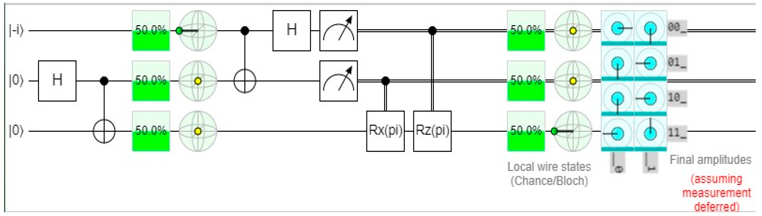
- —Relative phase between state components ;
Figure 3 illustrates the successful teleportation of from position A at the beginning of the circuit to Position B at the end of the circuit. State is observed at both positions, with a probability of of it being in state if it is measured. We obtain values of and for angles and , respectively. This quantum circuit is constructed and simulated using Quirk. However, the quantum-inspired teleportation circuit in this study is implemented in MATLAB R2023b, using quantum gates in matrix form. The teleportation of any random qubit state is perfectly performed. In other words, the probability amplitudes of state components and are reproduced. The relative phase between these state components is determined through the following steps:
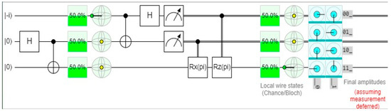
Figure 3.
Quantum teleportation circuit (Image generated using: https://algassert.com/quirk).
Step 1: Create a Bell state
The second and third qubit states are initialized to . A Hadamard gate is then applied to the second qubit, putting it in a superposition state, and then a controlled NOT gate is applied to the third qubit, with the second qubit being the controlled qubit. These operations create the state , which is one of the four Bell states:
Step 2: Perform an entanglement
Two or more quantum-entangled systems are correlated in such a way that their states cannot be described independently. In other words, the state of one quantum system is directly related to that of another system regardless of the distance between them.
In the present case, the random quantum state is entangled with the Bell state in Equation (27) by applying a controlled NOT gate to the second qubit, with the first qubit being the controlled qubit, and then a Hadamard gate is applied to the first qubit.
First, the tensor product between the first qubit from Equation (24) and the Bell state in Equation (27) is evaluated as follows:
The different components of Equation (30) can be expressed as follows:
Equation (30) can be expressed in full as
For greater understanding, Equation (35) is written in the following form:
Step 3: Measure quantum states
A quantum state is measured to determine its classical state. After this measurement, the quantum state that could be in a superposition state collapses into its basis state with the higher probability rate. In the present case, while measuring the first and second quantum states, the third qubit state is receiving the results in the form of the basis states of a two-qubit quantum system, which are .
Quantum measurements are irreversible; they destroy quantum information encoded in the quantum system, keeping only the classical information. To recreate the random qubit state, Pauli gates X and Z are applied to the third qubit state as follows.
If the third qubit receives the measurement result , then it performs the identity gate, which is equivalent to performing no operation:
If the third qubit receives the measurement result , then it performs the X gate, which swaps the states of and :
If the third qubit receives the measurement result , then it performs the Z gate, which changes the sign of :
If the third qubit receives the measurement result , then it performs the ZX gate, which swaps the states of and then changes the sign of :
After measuring the first and second qubits and then performing Pauli gates X and Z on the third qubit, is found in all cases, which is the random quantum state from Equation (24). The random qubit state from position A has thus been successfully teleported to position B.
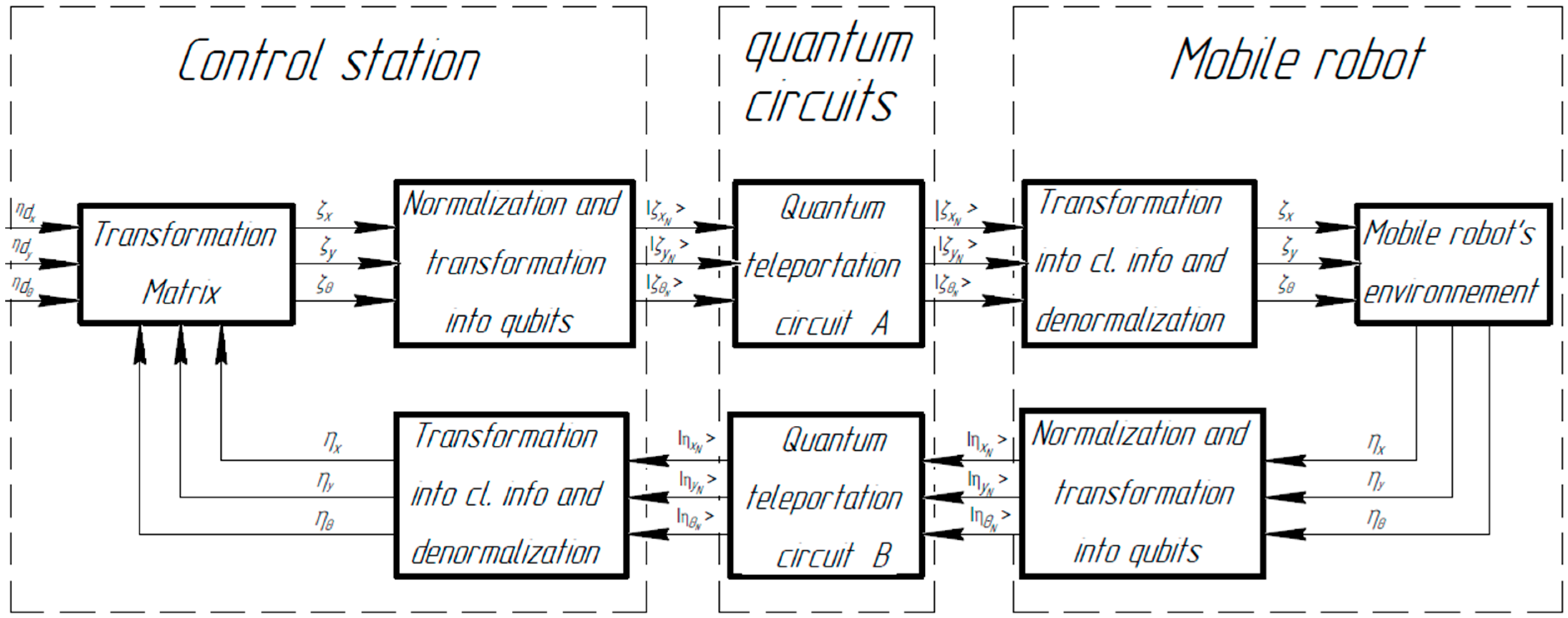
2.3. System Architecture
Our aim is to exchange velocity and position in the form of quantum information between the station and the robot. The proposed system consists of three independent parts: the control station, the quantum teleportation circuit, and the mobile robot, as depicted in Figure 4.
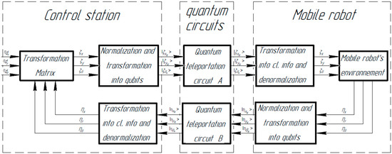
Figure 4.
Schematic of system architecture.
2.3.1. Control Station
The control station is the fixed part of this robotic system that interacts with users, enabling them to enter information on the trajectory to follow. It also allows the user to monitor the simulation. Before teleporting velocity input commands from Equation (6), they must be normalized, allowing them to easily be written as qubits. The nonholonomic longitudinal velocity is normalized using the following relationship:
The nonholonomic lateral velocity is normalized using
and the nonholonomic angular velocity is normalized using
where , , and are the maximum values of the nonholonomic longitudinal velocity, lateral velocity, and angular velocity, respectively.
The normalized velocity inputs are transformed into qubit states using the fact that the formula of any random qubit state can be represented as
For calculation simplicity, the angle is assumed to always be zero. To convert the normalized velocities into qubit states, we use the trigonometric identity
Writing , the normalized longitudinal velocity is expressed in qubit form as
the normalized lateral velocity is expressed in qubit form as
and the normalized angular velocity is expressed in qubit form as
2.3.2. Car-like Mobile Robot
The CLMR receives the data in quantum form. It is important to convert the data into classical information so that the robot can process them. This is performed through the denormalization of the teleported velocity input commands.
The teleported longitudinal velocity, lateral velocity, and angular velocity are denormalized using Equations (49) to (51), respectively.
After processing the teleported information, the robot starts moving according to Equation (23). This position data must be teleported to the control station to correct errors in the path following the normalization of actual positions with respect to the x-axis, y-axis, and , as follows:
The normalized positions are then transformed into qubit states to be teleported from the mobile robot to the control station (Equations (55)–(57)). In this process, the double-angle trigonometric identity for cosine is again used.
2.3.3. Quantum Teleportation Circuits
Quantum teleportation circuits can set a high-quality and secure connection, allowing the instantaneous transfer of data between the robot and its control station. Another advantage of quantum teleportation over classical wireless communication is the fidelity of the teleported data. For the proposed teleportation algorithm, Equation (30) is expressed in matrix form:
The random qubit state and second qubit state of the circuit are measured by searching for the largest probabilities, assuming that the measurement result of = 0 occurs when the probability of being in the classical state is greater than or equal to the probability of it being , or . The measurement result = 1 occurs when the probability of being in the classical state is less than the probability of it being . That is, .
Such as:
The probability of being in the classical state equals
The probability of being in the classical state equals
After the measurement, if the measured values of the random qubit state and the second qubit of the circuit are zero, then the following holds:
—Identity matrix.
The case where the measurement result of the random qubit state is 0 when the second qubit of the circuit is 1 is expressed as
—Pauli gate X in matrix representation.
The case where the measurement result of the random qubit state is 1 when the second qubit of the circuit is 0 is expressed as
—Pauli gate Z in matrix representation.
The measurement result of the random qubit state when the second qubit of the circuit is 1 is expressed as
In all four cases, the random qubit state is successfully teleported, showcasing the performance of the proposed quantum teleportation circuit.
During the feedback process to the control station, the control station receives data about positions in quantum form. To transform them into classical information, the denormalization of teleported positions is required. This is performed for the teleported positions with respect to the x-axis, y-axis, and angle using Equations (63)–(65), respectively.
The control station has the desired positions of the robot. Velocity inputs that depend on this information are sent to the mobile robot. Dynamic parameters, such as actuator dynamics, inertia, mass distribution, friction, and traction, and environmental factors influence the robot’s motion, resulting in actual positions that differ from the desired ones. Therefore, actual positions are used as feedback information to correct the errors in path following:
- —Teleported position error and teleported velocity error;
- —Desired position and actual teleported position;
- —Desired velocity and actual teleported velocity.
2.4. Simulation Setup
The simulation was conducted over 60 s. The CLMR model was implemented in MATLAB R2023b, assuming a robot length and width of 0.3 and 0.25 m, respectively. The mass and inertia were initialized to 10 kg and 0.1 kgm, and the optimal proportional and derivative control gains were fixed at Kp = 178.77 and Kd = 490, respectively.
3. Results and Discussion
3.1. Results
3.1.1. Circular Trajectory
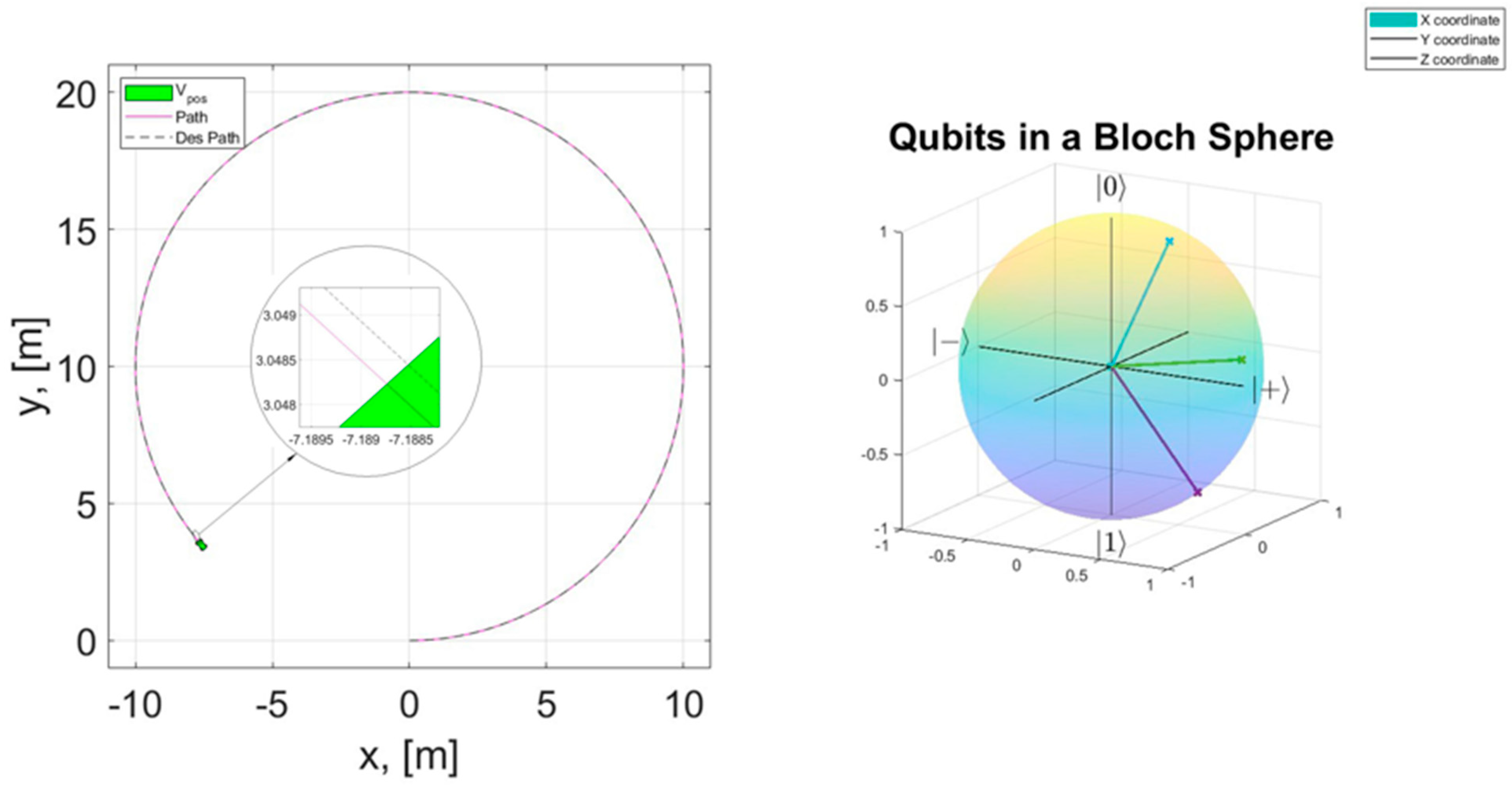
The desired trajectory for the robot to follow was defined as a circle with 20 m diameter. The environment was assumed to be flat and smooth, and the only constraints considered were the gravitational and inertial forces. Figure 5 depicts the simulation of the CLMR.

Figure 5.
Motion of car-like mobile robot (CLMR) following a circular trajectory.
The CLMR moves in the 2D x–y plane. The z-axis represents the angle between the robot’s longitudinal axis and the global x-axis. Visualizing the RMSE provides a way of evaluating how closely the robot follows the desired trajectory, with low RMSE values indicating that the robot’s trajectory closely matches the desired trajectory and high RMSE values indicating that the robot follows the desired trajectory but with substantial errors.
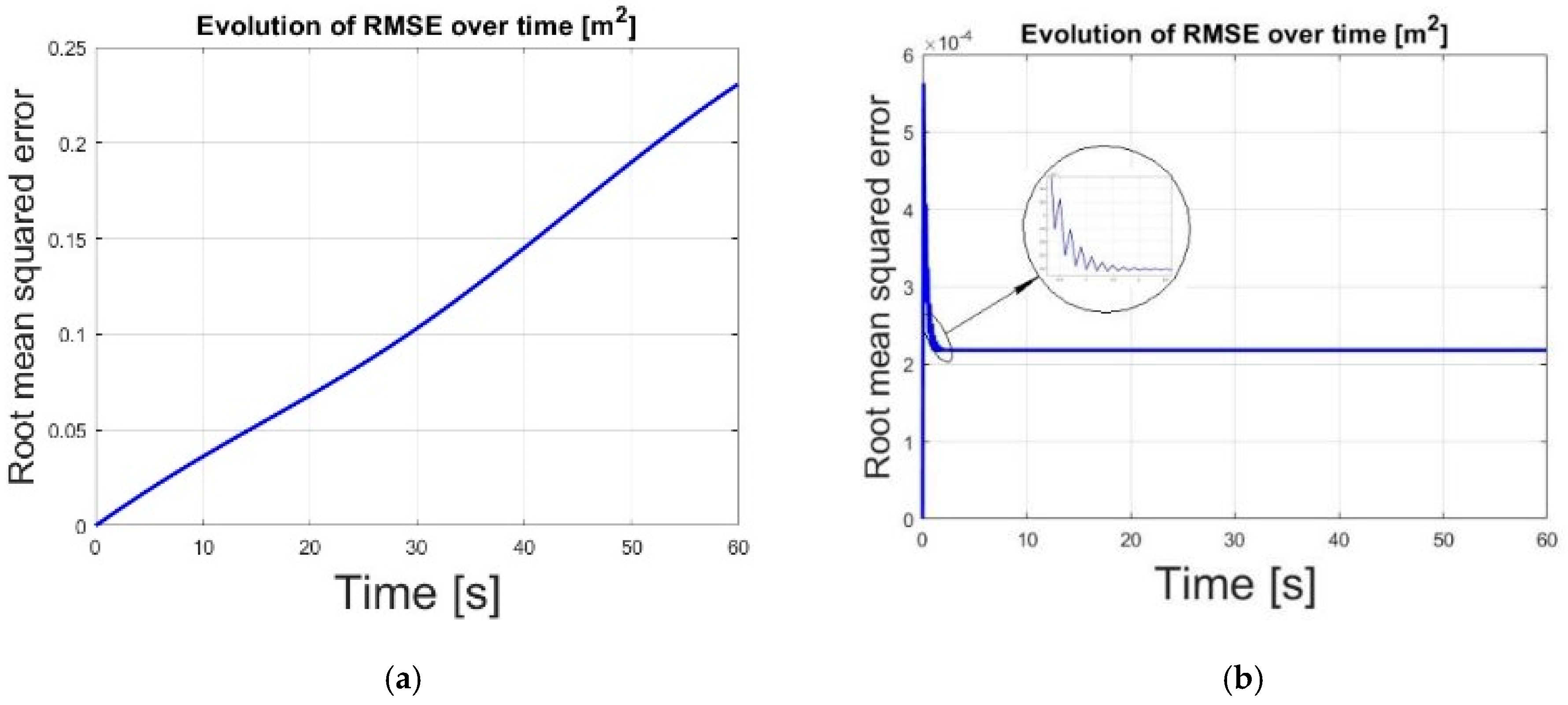
The results presented in Figure 6 highlight the significant role of the proportional and derivative control gains in effectively reducing and stabilizing the path-following error.

Figure 6.
Root mean square error (RMSE) with (a) Kp = 0, Kd = 0; (b) Kp = 178.77, Kd = 490.
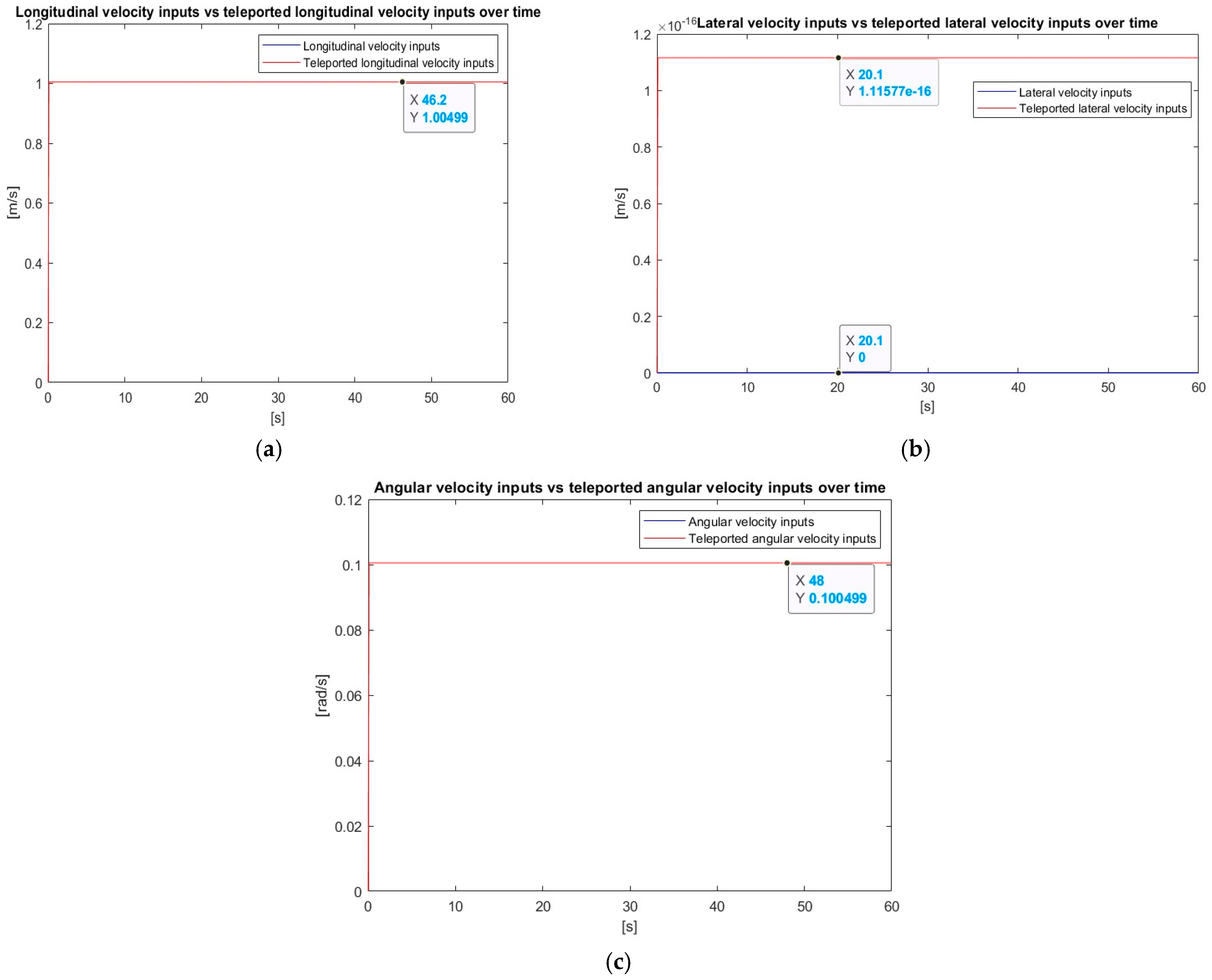
To textually teleport each qubit state, the quantum circuit must destroy it at the input of the circuit and then restore the identical quantum state by reproducing the probability amplitudes of state components and the relative phase between them. To prove this statement, the performance of the proposed quantum teleportation circuit algorithm was evaluated by comparing time graphs of each data until the data are destroyed and teleported with the graphs of the data after teleportation. Figure 7 illustrates the correspondence between the graphs of the input data and the corresponding transmitted data.
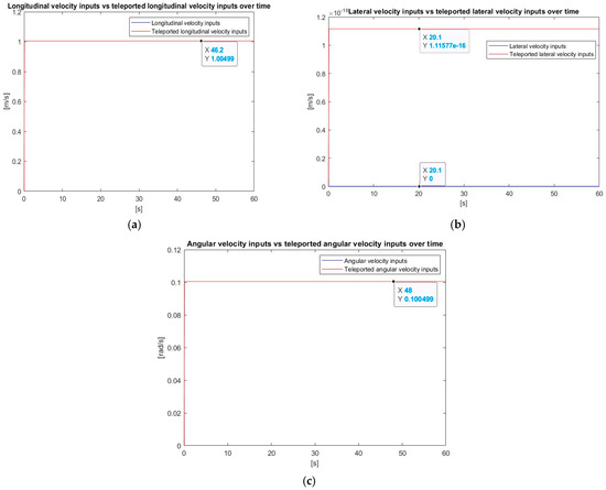
Figure 7.
Longitudinal, lateral, and angular velocities over time for the circular trajectory: real versus teleported data. (a) Linear longitudinal velocity. (b) Linear lateral velocity. (c) Angular velocity over time.
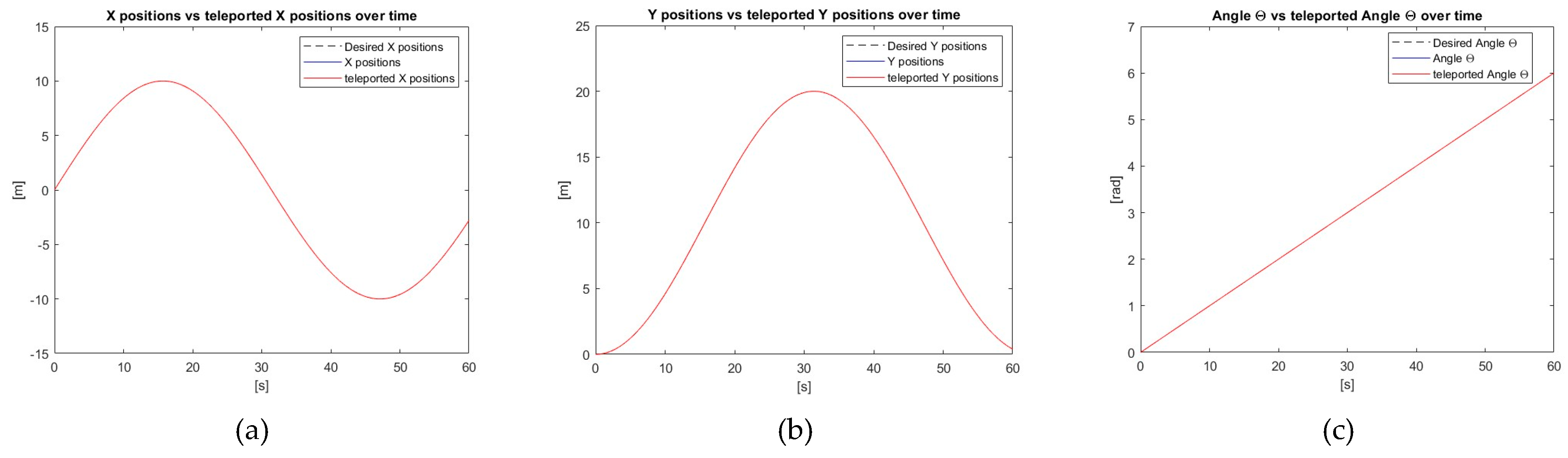
The information about the velocities of the CLMR provided in Figure 7 is teleported from the control station to the robot. Similarly, we compared the robot’s positions before and after teleportation to verify the exact teleportation of data. Figure 8 shows the precision of the correspondence between actual and teleported positions, demonstrating the high quality of our implemented quantum computing circuits.
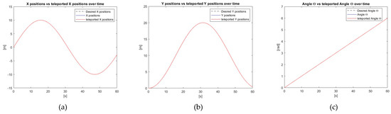
Figure 8.
x-, y-, and z-positions of circular trajectory: (a) x-position, (b) y-position, and (c) z-position.
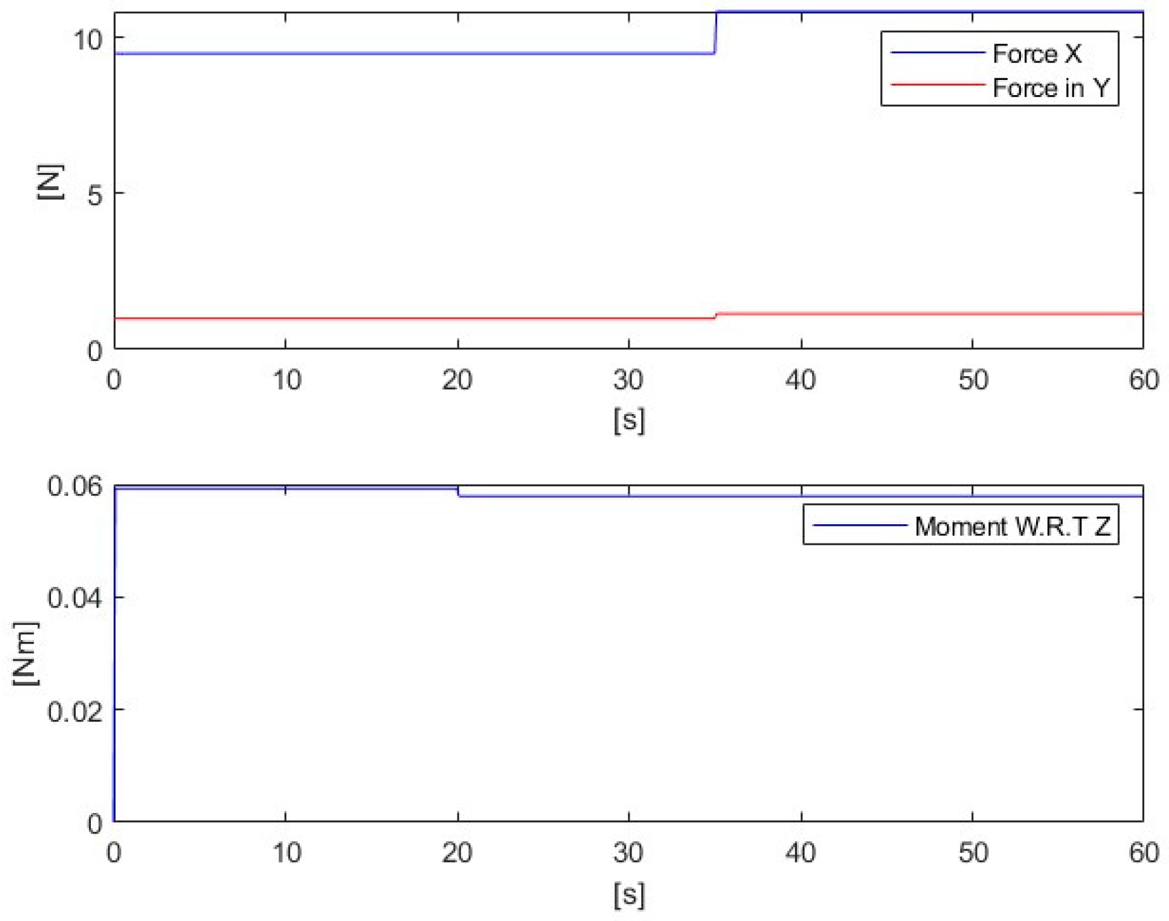
We concluded the experiment by testing the robot’s robustness by introducing errors. After 20 s, the robot’s inertia was reduced by 10%. Then, the robot’s mass was increased by 15% at 35 s. The introduction of these errors did not significantly affect the trajectory, because the robot’s controller compensated for the forces and momentum applied to the robot, as depicted in Figure 9.

Figure 9.
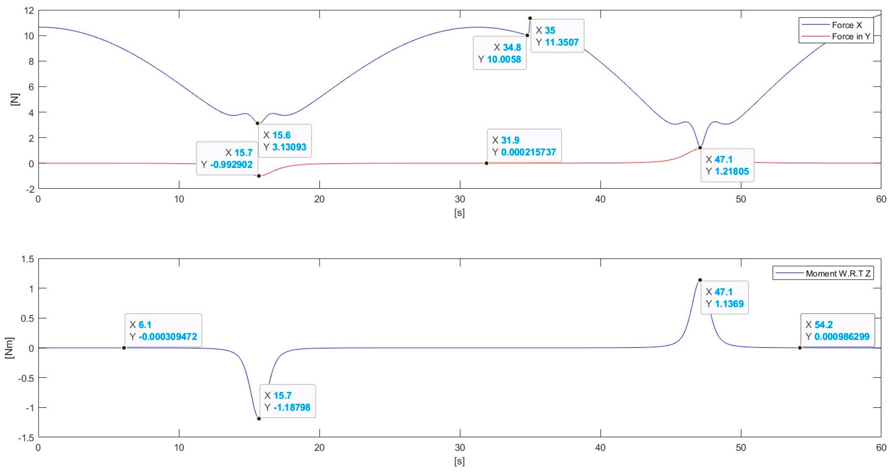
Forces and momentum applied to the robot over time for the circular trajectory.
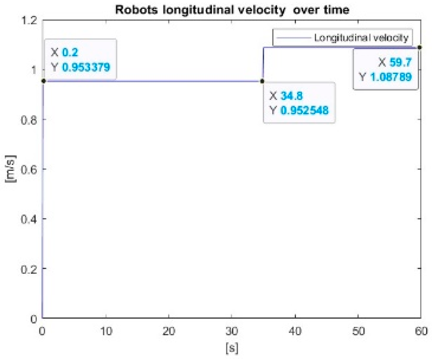
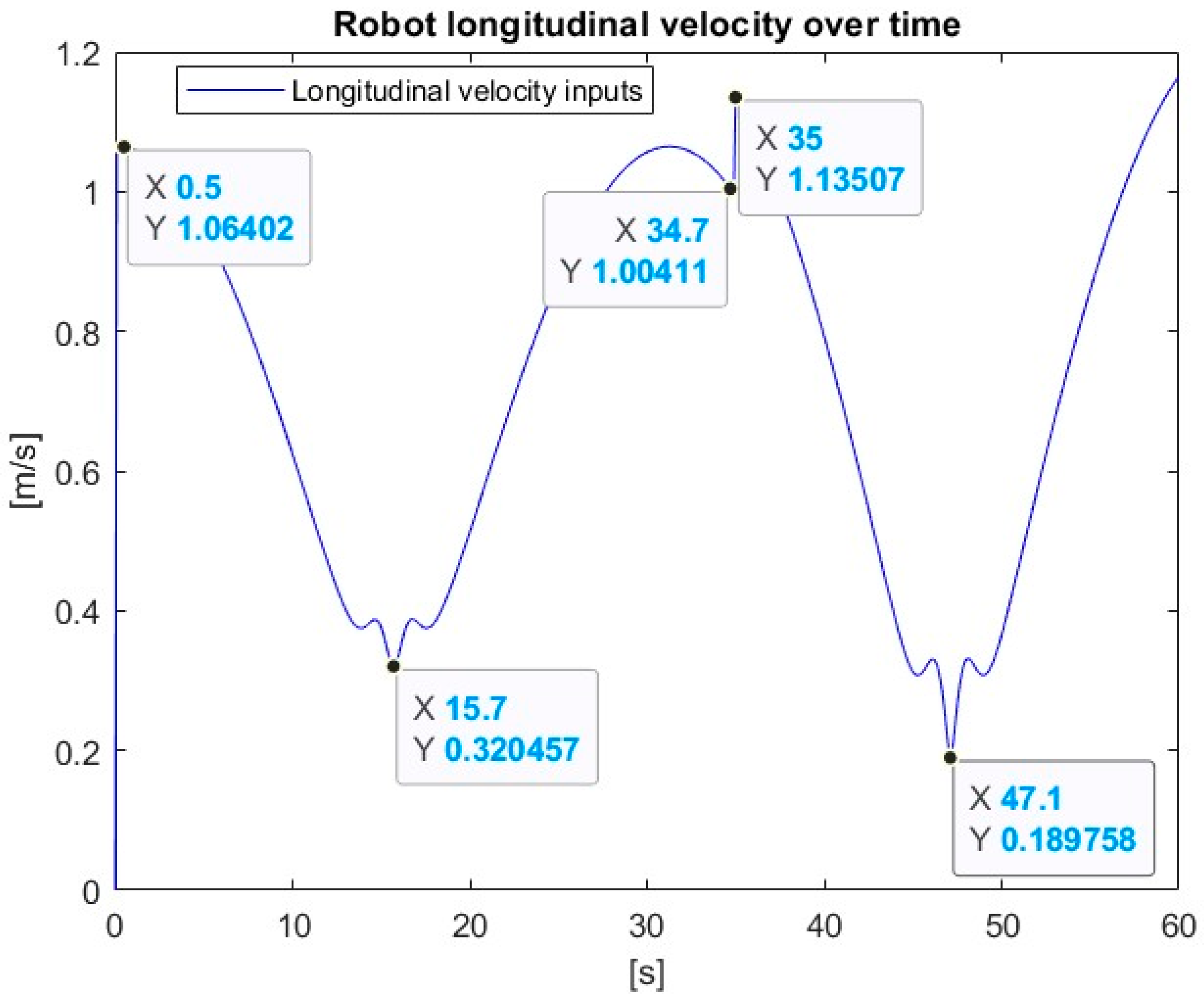
The compensations of the force and momentum in this test had a considerable impact on the linear velocity of the robot, as depicted in Figure 10.

Figure 10.
Linear velocity after introducing errors for the circular trajectory.
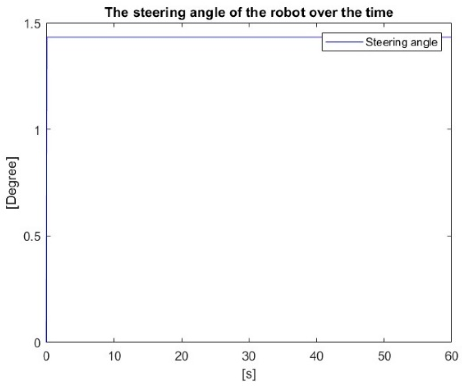
As shown in Figure 11, the steering angle remained constant throughout the simulation. This adaptation of velocities demonstrates the robot’s ability to adapt to changes while maintaining its path-following performance.
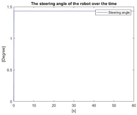
Figure 11.
Steering angle of robot for the circular trajectory.
3.1.2. Sine Wave Trajectory
This simulation was conducted in a flat and smooth environment, where the only constraints considered were the gravitational and inertial forces. Figure 12 provides more insight into the simulation of the CLMR following a sine wave trajectory with an amplitude and period of 10 m.
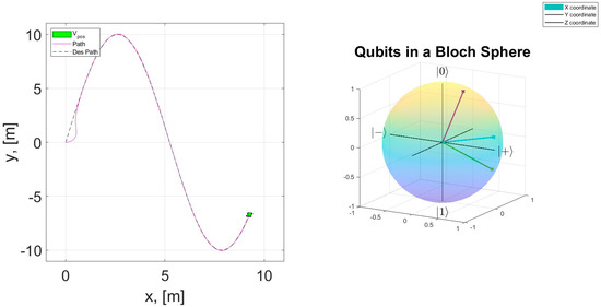
Figure 12.
Motion of CLMR following a sine wave trajectory.
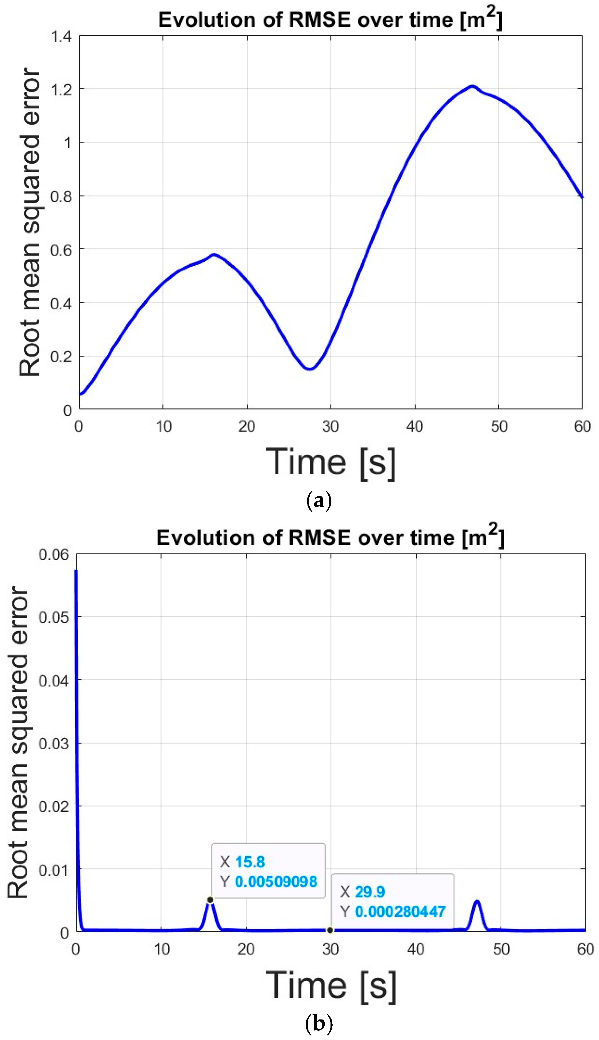
The CLMR was able to track the desired trajectory reasonably well using the optimized parameters. The results shown in Figure 13 demonstrate the significant role of the proportional and derivative control gains in effectively reducing and stabilizing errors in trajectory tracking.
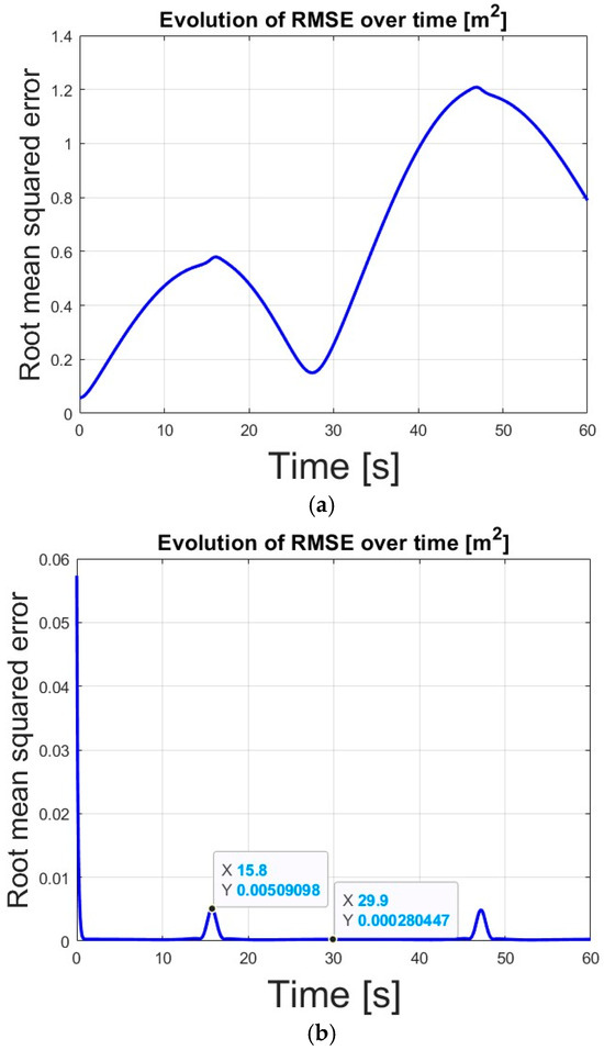
Figure 13.
RMSE with (a) Kp = 0, Kd = 0; (b) Kp = 144.99, Kd = 275.2.
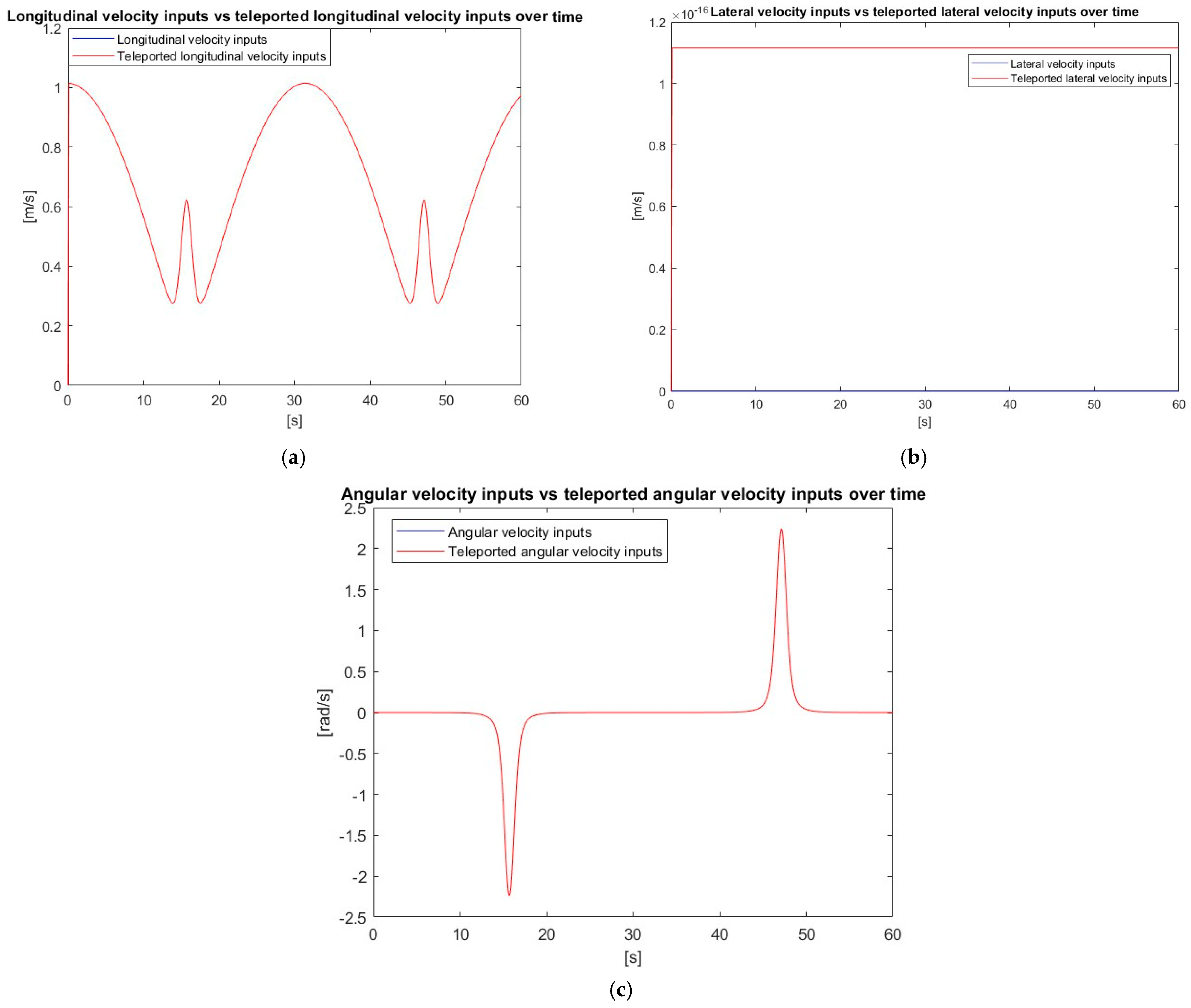
The correspondence between the graphical representations of the velocity input data and the corresponding transmitted data is illustrated in Figure 14.

Figure 14.
Longitudinal, lateral, and angular velocities over time for the sine wave trajectory: real versus teleported data. (a) Linear longitudinal velocity. (b) Linear lateral velocity. (c) Angular velocity over time.
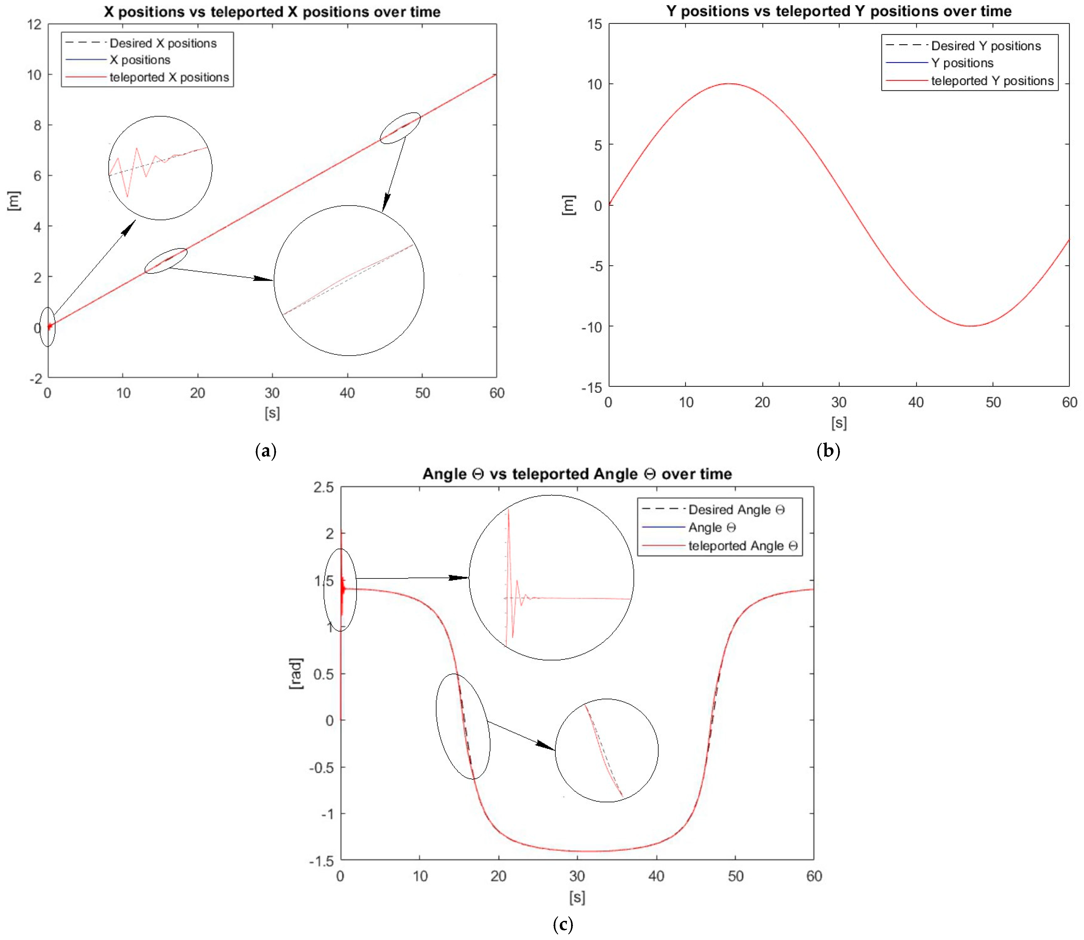
Figure 15 shows the precision of the correspondence between the real and teleported positions, which verifies the high quality of the quantum computation circuits used.
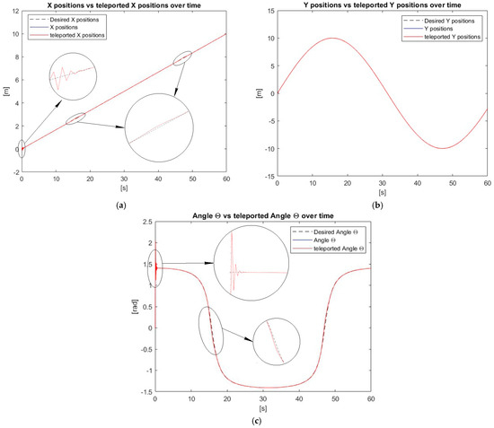
Figure 15.
x-, y-, and z-positions for the sine wave trajectory: (a) x-position, (b) y-position, and (c) z-position.
We also tested the robustness of the robot for the sinusoidal trajectory by introducing errors. After 20 s, the robot’s inertia was reduced by 30%. Then, the robot’s mass was increased by 15% at 35 s. The introduction of these errors had no significant impact on the robot’s trajectory, because the robot controller compensated for the forces and momentum applied to the robot, as shown in Figure 16.
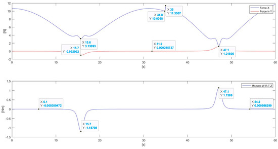
Figure 16.
Forces and momentum applied to the robot over time for the sine wave trajectory.
These compensations in the robot robustness test had a considerable impact on the robot’s linear velocity and steering angle, as shown in Figure 17 and Figure 18, respectively.
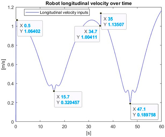
Figure 17.
Linear velocity after introducing errors for the sine wave trajectory.
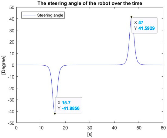
Figure 18.
Robot’s steering angle for the sine wave trajectory.
As shown in Figure 18, the steering angle in the robustness test remained the same as that in the simulation steering graph without the robustness test. This adaptation of the speeds demonstrates the robot’s ability to adapt to changes while maintaining its path-following performance.
3.1.3. Linear Trajectory
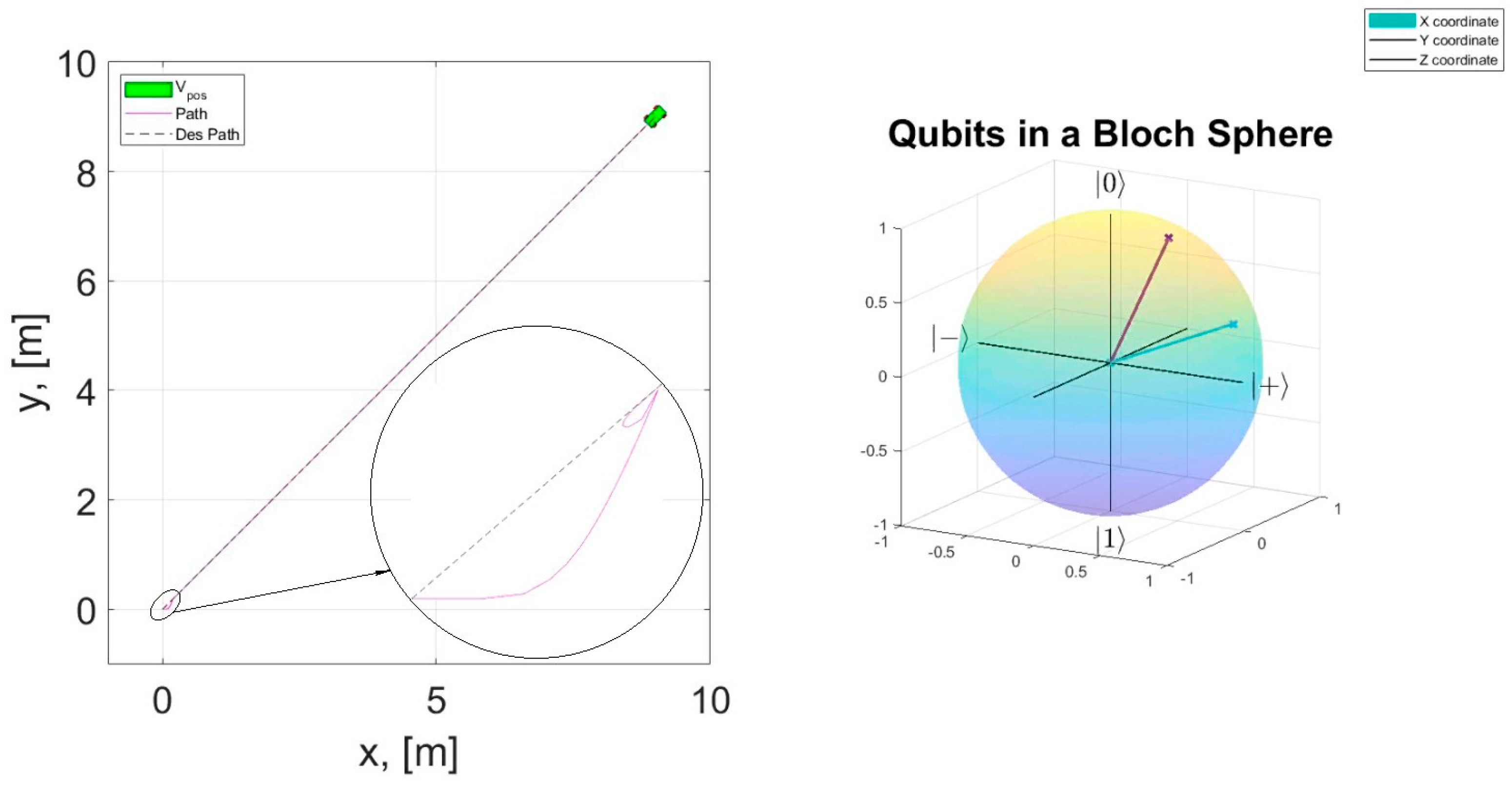
This simulation was also conducted in a flat and smooth environment, where the only constraints considered were gravitational and inertial forces. Figure 19 provides more insight into the simulation of the CLMR following a linear trajectory at an angle of 45° from the global x-axis.
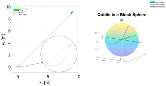
Figure 19.
Motion of CLMR following a linear trajectory.
The CLMR follows the desired trajectory reasonably well using the optimized parameters. Figure 20 shows how the proportional and derivative control gains effectively reduced and stabilized the errors in trajectory tracking.
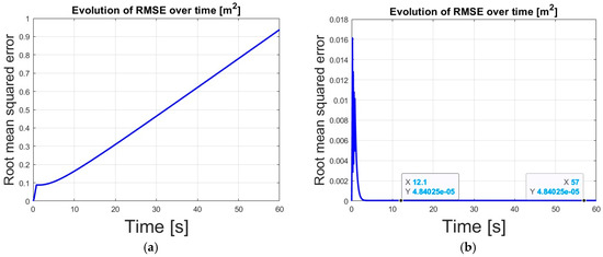
Figure 20.
RMSE with (a) Kp = 0, Kd = 0; (b) Kp = 178.77, Kd = 411.7.
The correspondence between the graphical representations of the velocity input data and the corresponding transmitted data is illustrated in Figure 21.

Figure 21.
Longitudinal, lateral, and angular velocities over time for linear trajectory: real versus teleported data. (a) Linear longitudinal velocity. (b) Linear lateral velocity. (c) Angular velocity over time.
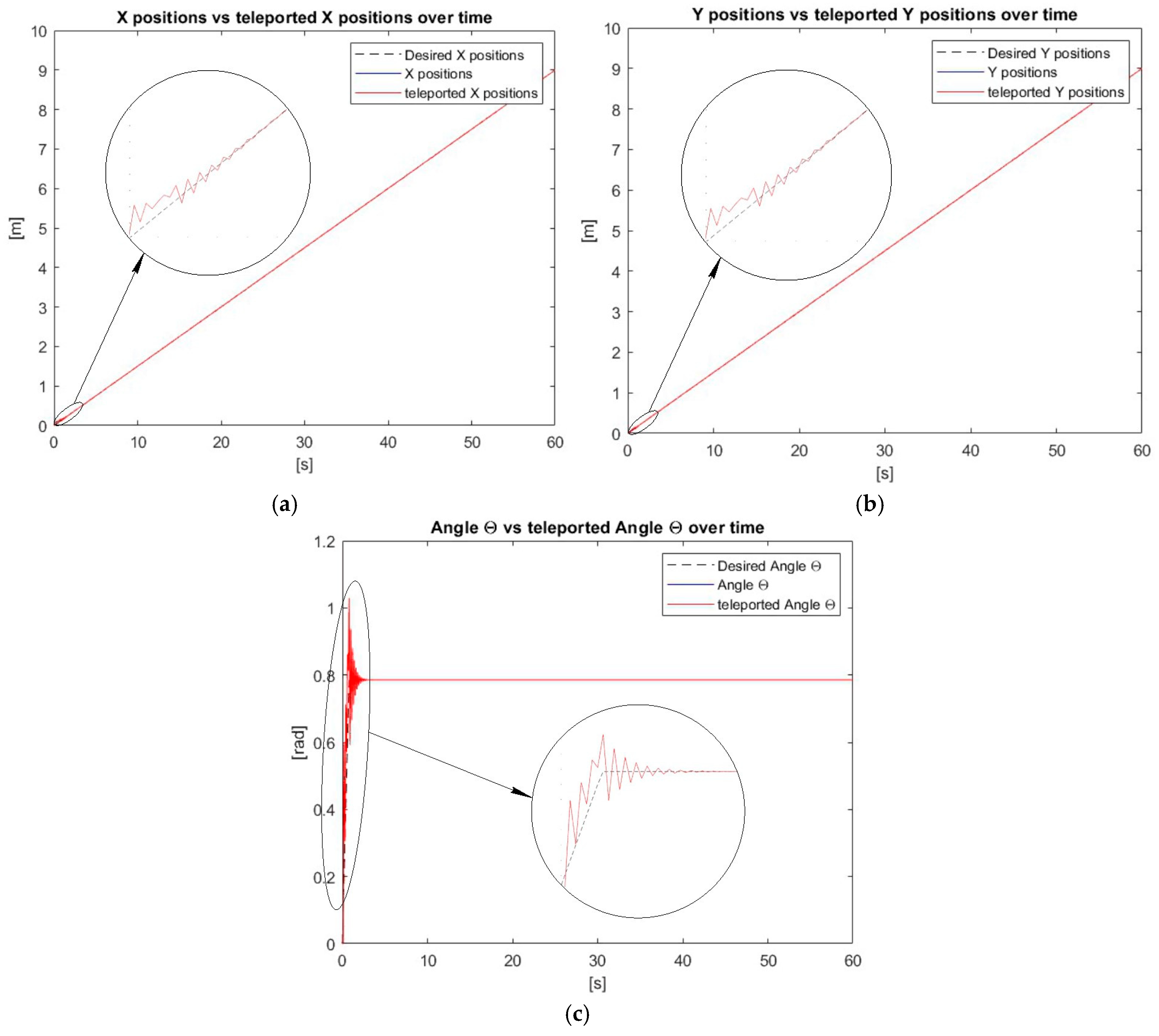
Figure 22 illustrates the high quality of the quantum computation circuits used by showing the precision of the correspondence between the real and teleported positions.
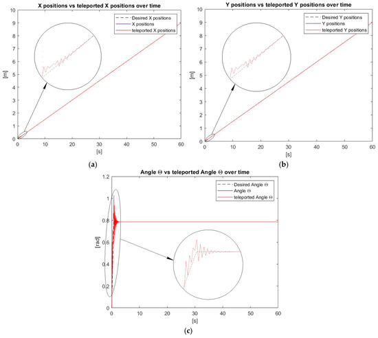
Figure 22.
x-, y-, and z-positions for the linear trajectory: (a) x-position, (b) y-position, and (c) z-position.
We also tested the robot’s robustness by introducing an error after 20 s by reducing the robot’s inertia by 30% and another error at 35 s by increasing its mass by 15%. These errors had no significant impact on the trajectory, because the robot controller compensated for the forces and momentum applied to the robot, as shown in Figure 23.
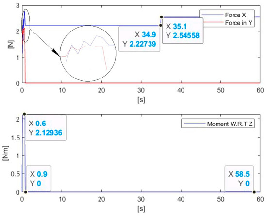
Figure 23.
Forces and momentum applied to the robot over time for the linear trajectory.
These compensations in the robot robustness test had a considerable impact on the robot’s linear velocity and steering angle, as shown in Figure 24 and Figure 25, respectively.

Figure 24.
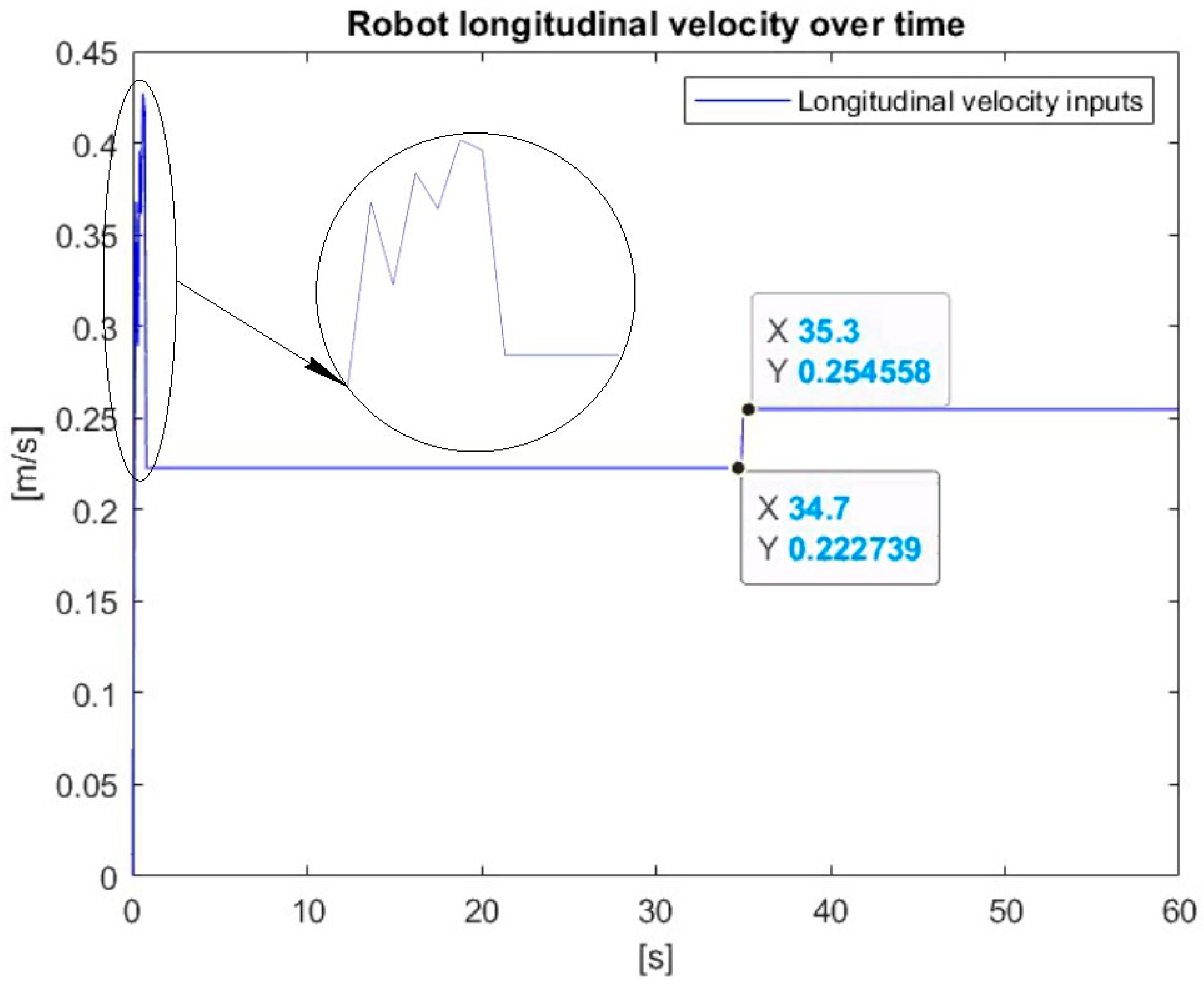
Linear velocity after introducing errors for the linear trajectory.
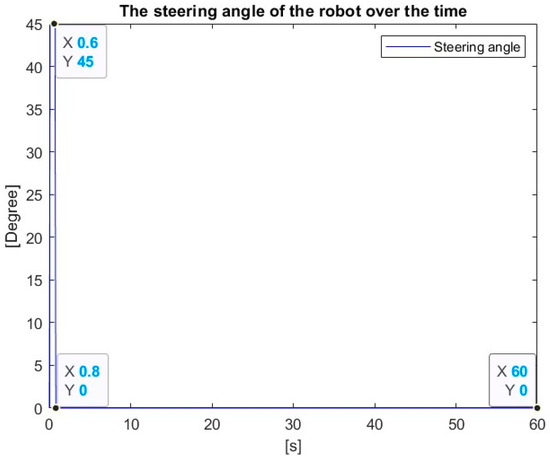
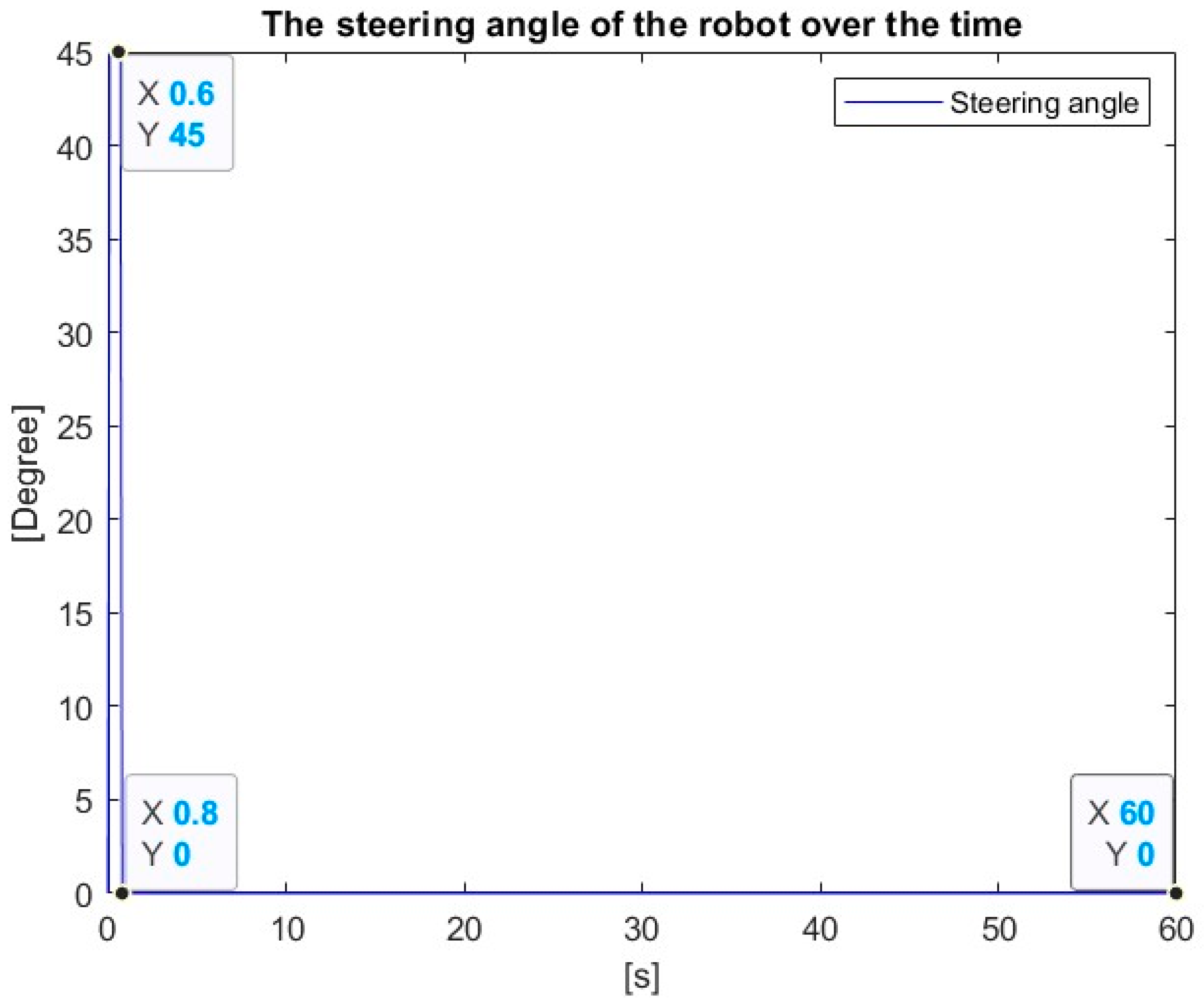
Figure 25.
Robot’s steering angle for the linear trajectory.
As shown in Figure 25, the steering angle abruptly increased from 0 to 45° in 0.1 s, then decreased to 0° at 0.8 s and remained constant until the end of the simulation. Similarly to in the previous trajectories, the robot adapted its speeds to changes while maintaining its path-following performance.
3.2. Discussion
3.2.1. Circular Trajectory
The quantum-implemented circuit enabled the teleportation and exchange of data between the robot and its control station. The Bloch sphere introduced in Figure 5 allows the robot’s position with respect to the x-, y-, and z-axes to be observed in the quantum form by visualizing the qubits moving in the Bloch sphere as the robot moves in its environment. The trajectory followed by the CLMR may differ from the desired trajectory, introducing errors in the path tracking. These errors are mainly due to data-processing faults by the controller and other dynamic constraints, such as the effect of gravitational and inertial forces on the robot. These errors were calculated as the squared difference between the desired trajectory and the trajectory followed by the robot. This information allowed the calculation of the mean square error, which quantifies the deviation between the desired and actual trajectories. Figure 6a demonstrates that without optimization, the error exponentially increased from 0 to 0.23 m2 at the end of the simulation, whereas Figure 6b shows that when Kp and Kd were optimized, the error increased from zero to a maximum of 5.63 × 10⁻⁴ m2 at 0.1 s before decreasing and stabilizing at 2.18 × 10⁻⁴ m2 from 2.3 s. This represents a marked reduction of the error. Although it was important to stabilize the error, which increased exponentially, the primary aim was to teleport and exchange the input and output data between the mobile robot and its control station using quantum computing techniques. Figure 7a shows a comparison between the input and teleported linear longitudinal velocities. Both velocities increased from 0 to 1.005 m/s in 0.1 s then remained constant until the end of the simulation. For the lateral velocity, the nonholonomic robot did not have any forces acting on its side. The teleported lateral velocity increased from zero and stabilized at 1.1 × 10⁻¹⁶ m/s, as depicted in Figure 7b. The lateral velocity before teleportation remained at zero throughout the simulation. Since the difference between these two values is minor, perfect teleportation of the lateral velocity can be assumed. Figure 7c also shows the perfect correspondence between the input and teleported angular velocities. At the beginning of the simulation, both angular velocities increased from zero to approximately 0.1005 rad/s at 0.1 s then remained constant until the end of the simulation. When the input velocities were teleported from the control station to the robot’s controller, the robot started moving and collecting data about its position with respect to the x-, y-, and z-axes.
In the test of the robot robustness, the robot’s longitudinal force was 9 N and its moment of inertia was zero at the start of the simulation. At 0.1 s, the moment of inertia abruptly increased to 0.06 Nm. After 20 s, the robot’s moment of inertia with respect to the z-axis decreased to 0.0579 Nm. At 35 s, the force applied to the robot’s wheels increased to 10.8531 N and the linear velocity slightly decreased from 0.953379 to 0.952548 m/s. Then between 34.8 and 35.1 s, it suddenly increased to 1.08789 m/s then remained stable until the end of the simulation. The CLMR updated its velocity at 0.1 s while keeping the steering angle constant at 1.4321°, as shown in Figure 11.
3.2.2. Sine Wave Trajectory
Figure 12 shows the position of the robot relative to the x-, y-, and z-axes on a 2D plane and in the Bloch sphere, where the qubits represent the different positions when the robot moves in its environment. Figure 13a shows the exponential growth of the error from 0.057 m2 at 16 s to 0.789 m2 at the end of the simulation. The initial error was nonzero because the robot started moving from a perpendicular position to the desired trajectory, then the error increased while oscillating to its first maximum of 0.579 m2 at 16 s, then decreased to a local minimum of 0.151 m2 at 27.6 s before reaching a global maximum of 1.21 m2 at 46.8 s. Figure 13b shows that when Kp and Kd were optimized, the RMSE decreased from 0.057 to 0.0002558 m2. Similarly to Figure 13a, Figure 13b depicts oscillations in the RMSE at 16 and 46.8 s, with local maxima of 0.005 m2. At these two times, the robot was located at the peak amplitudes of the sine wave trajectory. Figure 14a shows a comparison between the input and teleported linear longitudinal velocities. Both velocities increased from initial values of zero to 1.013 m/s at 0.1 s, which was the global maximum value reached at 0.1 and 30 s. The longitudinal velocity fluctuated during the simulation, with local minima of 0.276 m/s at 14, 18, 45, and 49 s and local maxima of 0.622 m/s at 15.5 and 45 s. For the lateral velocity, the nonholonomic robot did not have any forces acting on its side. The teleported lateral linear velocity increased from zero and stabilized at 6.713 × 10⁻²⁰ m/s, as depicted in Figure 14b. The lateral velocity before teleportation remained zero throughout the simulation. Since the difference between these two values is minor, perfect teleportation of the lateral velocity can be assumed. The perfect correspondence between the angular velocity and the teleported angular velocity can be seen in Figure 14c. At the beginning of the simulation, both angular velocities were zero. They then decreased to −2.242 rad/s between 11.5 and 15.5 s, where the negative value indicates resistance to the car’s rotation while steering to the left side. Then the angular velocity slowly increased to zero between 15.5 and 19.5 s. After that, the angular velocity remained at zero until 43.5 s. It then started increasing, reaching 2.242 rad/s at 47.2 s, where the positive value indicates resistance to the car’s rotation while steering to the right side. The velocity then slowly decreased to zero between 47.2 and 50 s, then remained at zero until the end of the simulation. The graph of the robot’s longitudinal force presented in Figure 16 is a transform of the sinusoidal function, starting at an amplitude of 10.646 N and slowly decreasing to a local minimum of 3.131 N at 15.6 s. The longitudinal force then recovered to 10.646 N at 30.1 s. The global minimum of 1.218 N occurred at 47.1 s, after which the longitudinal force increased to 10.189 N at the end of the simulation. To compensate for the abrupt increase in the mass at 35 s, the controller increased the longitudinal force to 11.351 N. A graph of the robot’s moment of inertia is also presented in Figure 16; its value is mostly zero with two fluctuations resulting in a minimum of −1.188 Nm at 15.6 s and a maximum of 1.137 Nm at 47.1 s, where the negative (positive) value indicates resistance to the car’s rotation while steering to the left (right) side. The difference between the absolute values of these two moments of inertia demonstrates the behavior of the controller during the robustness test. The graph of the robot’s lateral force behaved similarly to that of the robot’s moment of inertia; it mostly had a value of zero with two oscillations resulting in peaks at 15.6 and 47.1 s. The first oscillation resulted in a local minimum of −0.987 N, whereas the second oscillation increased the force from 0 to 1.14 N, showcasing the effectiveness of the controller in overcoming errors introduced in the robustness test. Figure 17 depicts the linear velocity of the robot. The velocity increased from 0 to 1.064 m/s at 0.1 s, decreased to a local minimum of 0.320 m/s at 15.7 s, and increased to another local maximum at 30 s, which was followed by a global minimum of 0.19 m/s at 47.1 s. The maximum velocity of 1.15 m/s was achieved at the end of the simulation. The CLMR updated its velocity while the steering angle.
3.2.3. Linear Trajectory
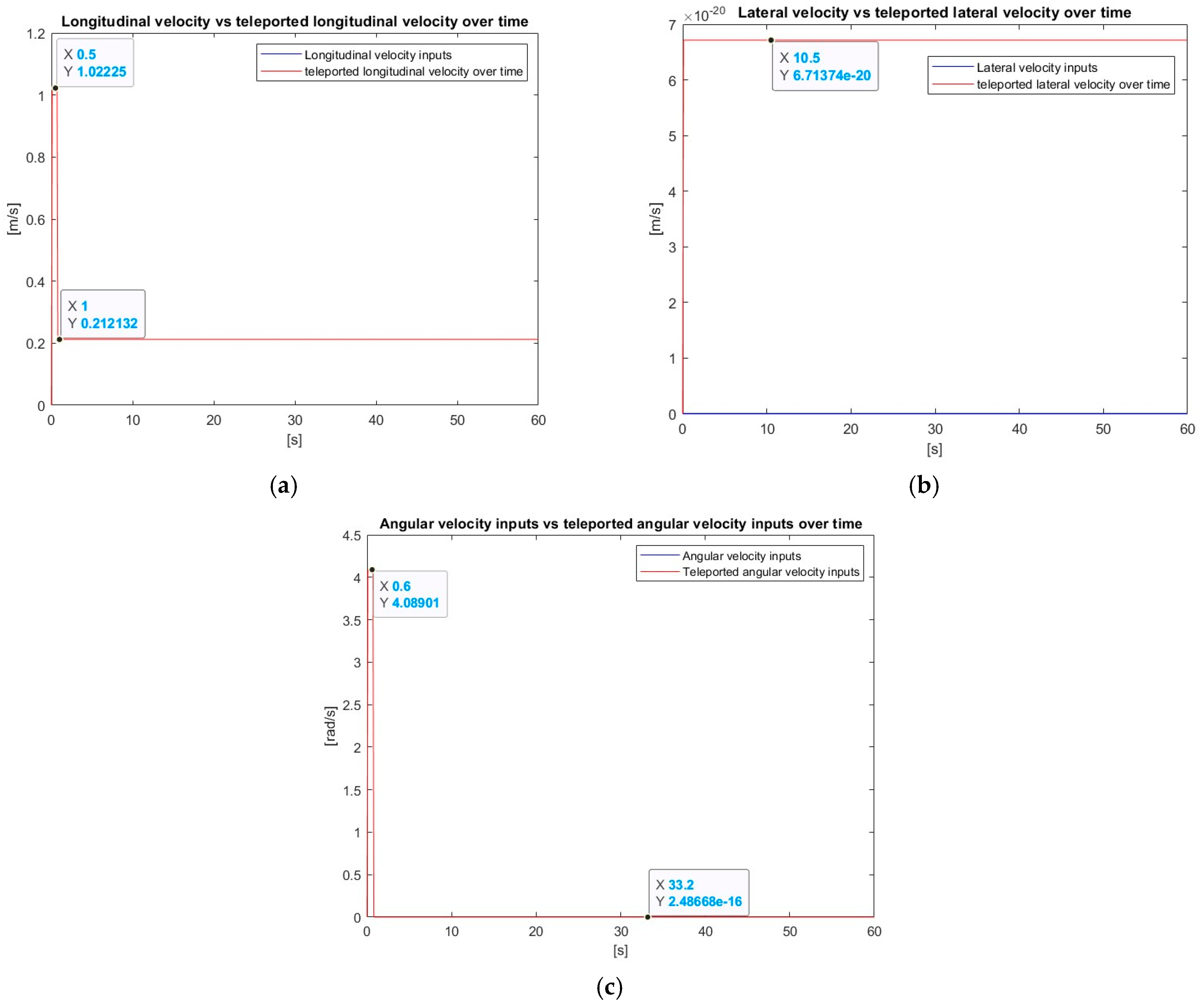
Figure 19 shows the robot’s motion along with the Bloch sphere, where the three qubits represent the robot’s positions relative to the x-, y-, and z-axes on a 2D plane. Although the initial position of the robot made an angle of with the desired trajectory, using the optimized Kp and Kd, the robot was able to improve its position to match the desired trajectory. As shown in Figure 20a, the RMSE increased almost linearly from 0 to 0.945 m2 during the simulation when the robot did not receive any feedback for corrections. For the optimized PD parameters, the RMSE increased from 0 to 0.016 m2 in the first 0.2 s, then decreased while oscillating until it stabilized at a value of 4.84 × 10⁻⁵ m2 at 5 s (Figure 20b). This stabilization was due to accurate velocity data teleported from the control station to the robot’s controller. Figure 21a depicts a comparison between the input and teleported linear longitudinal velocities. Both longitudinal velocities increased from 0 to 1.022 m/s at 0.1 s. Then at 0.5 s, they decreased, reaching 0.21 m/s at 1 s. They then remained constant for the remainder of the simulation. The teleported lateral velocity increased from 0 to 6.713 × 10⁻²⁰ m/s at the start of the simulation, then remained at this value, as shown in Figure 21b, whereas the lateral velocity before teleportation remained at zero throughout the simulation. Because of the small difference between these values, perfect teleportation of the lateral velocity can be assumed. Figure 21c shows the perfect correspondence between the angular velocity and the teleported angular velocity. Both angular velocities increased from 0 to 4.089 rad/s in 0.1 s, then from 0.5 to 1 s decreased to 2.48 × 10⁻¹⁶ rad/s then remained constant for the remainder of the simulation. Figure 22 shows the precision of the correspondence between the real and teleported data for the x-, y- and z-positions. This affirms the precision of the correspondence between the real and teleported positions. The graphs in Figure 22a,b have similar shapes; they present the robot’s displacement relative to the global x- and y-axes. The robot’s teleported position matches the position before the teleportation. Figure 22c shows the teleported displacement of the robot in term of . The values before and after the teleportation were identical. increased from zero to the global maximum of 1.09 rad at 0.8 s while fluctuating, then stabilized at 0.786 rad at 3.2 s, a value maintained until the end of the simulation. Figure 23 shows that in the robustness test, the longitudinal force oscillated while increasing to a global maximum of 2.794 N at 0.6 s, before rapidly decreasing and stabilizing at 2.227 N at 1 s. This value was maintained until 35 s, when the longitudinal force jumped to 2.546 N to compensate for the error in the mass. This value was maintained until the end of the simulation. The lateral force was zero, except in the first 0.6 s, when it increased while oscillating to a global maximum of 2.12 N before dropping to zero for the remainder of the simulation. This value of 2.12 N was noise due to the sudden simultaneous increase in the moment of inertia to 2.13 Nm, which then returned to zero for the remainder of the simulation. Thus, the error introduced in the moment of inertia did not require compensation, as the robot moved in a straight line. Figure 24 shows that the longitudinal velocity increased while oscillating to a global maximum of 0.427 m/s at 0.6 s, before stabilizing at 2.227 m/s at 1 s. This value was maintained until 35 s, when the velocity jumped to 2.546 m/s to compensate for the error in the mass. The velocity remained at this value until the end of the simulation. The CLMR updated its velocity while the steering angle increased from 0 to in the first 0.7 s then returned to zero until the end of the simulation, as shown in Figure 25.
4. Conclusions
In this study, we simulated the dynamic movement of a CLMR, which was identified by its dimensions, mass, inertia, and steering angle and operated in an environment simulated using a specified coefficient of viscosity. In the first phase of this study, we compared the robot’s actual trajectory with a predetermined trajectory. The dynamic constraints of the robot and the viscosity of the environment provided substantial challenges in achieving this objective. To overcome these challenges, we designed a PD controller with optimized parameter values. The improvement of the controller’s parameters reduced and stabilized the RMSE.
The primary purpose of this study was to remotely exchange data between the control station and the CLMR by employing a quantum teleportation protocol that employed a quantum teleportation circuit designed using Quirk. This circuit, which consisted of quantum gates such as Hadamard and Pauli gates, was able to completely teleport any qubit state. Before developing a quantum teleportation circuit in MATLAB, we devised mathematical formulas to help comprehend the mechanism of qubit teleportation. To transfer data such as the robot’s velocity and position, it was necessary to translate these values into qubit form. At the control station, the user inputs the trajectory as differential equations. These equations and the Jacobian matrix are used to calculate the implicit velocity input command. After determining the velocity input, the control station normalizes them before converting them to quantum representation using trigonometric calculations. This novel approach enables the transmission of velocity data from the control station to the mobile robot. After receiving the data, the robot performs the reverse process: it converts the quantum form into normalized values before computing the real values so that they can be processed and applied to the robot’s wheels. A similar teleportation method is used to return the robot’s current position to the control station, allowing for the analysis of discrepancies between the desired and actual positions (position errors) and differences between the target and current velocity (velocity errors). These errors and the controller parameters are required to calculate the control command to reduce and stabilize the RMSE, allowing the robot’s real trajectory to match the desired trajectory.
We concluded our experiment by assessing the system’s robustness by changing the mass and inertia of the robot at different times. The steering angle remained constant, whereas the velocity, forces, and moment of inertia changed to compensate for the changes in mass and inertia. A comparison of the original data and the teleported revealed their high similarity, demonstrating that the proposed teleport protocol performed flawlessly even in the test for robustness.
To address the lack of quantum computers owing to their construction and maintenance costs, our future plans include the construction of actual quantum teleportation circuits to drive physical robots with the goal of considerably improving their operational efficiency and responsiveness. The findings of this study could promote the use of quantum teleportation circuits for securely exchanging data between robotic systems, overcoming the limitation of classical wireless communication media, such as electromagnetic waves and Wi-Fi transfer encoded signals, which are often affected by noise and interference in adverse environments and may also be attenuated in the case of a large distance between a mobile robot and its control station. These signals are also vulnerable to interception and hacking by malicious parties. Quantum teleportation could resolve these issues by using quantum entanglement to instantaneously share data regardless of the distance between the station and the mobile robot, with the quantum measurement principle ensuring the robustness of the data to interception.
Author Contributions
J.N. contributed to methodology, investigation, formal analysis, writing editing of the original draft, and visualization. N.Z. contributed to providing resources, supervision, project administration, formal analysis, review and editing of the original draft, funding acquisition, and visualization. M.T. contributed to conceptualization, formal analysis, review and editing of the original draft, and visualization. All authors have read and agreed to the published version of the manuscript.
Funding
This work was financially supported by NSERC Canada.
Data Availability Statement
All used data are available within the manuscript.
Conflicts of Interest
The authors declare no conflicts of interest.
References
- Numbi, N.Z.; Tadjine, M. Quantum Particle Swarm Optimisation Proportional–Derivative Control for Trajectory Tracking of a Car-like Mobile Robot. Electronics 2025, 14, 832. [Google Scholar] [CrossRef]
- Gehlot, V.P.; Balas, M.J.; Quadrelli, M.B.; Bandyopadhyay, S.; Bayard, D.S.; Rahmani, A. A Path to Solving Robotic Differential Equations Using Quantum Computing. J. Auton. Veh. Syst. 2022, 2, 031004. [Google Scholar] [CrossRef]
- Lathrop, P.; Boardman, B.; Martínez, S. Quantum Search Approaches to Sampling-Based Motion Planning. IEEE Access 2023, 11, 89506–89519. [Google Scholar] [CrossRef]
- Atchade-Adelomou, P.; Alonso-Linaje, G.; Albo-Canals, J.; Casado-Fauli, D. qRobot: A Quantum Computing Approach in Mobile Robot Order Picking and Batching Problem Solver Optimization. Algorithms 2021, 14, 194. [Google Scholar] [CrossRef]
- Koshelev, K.V.; Nikolaeva, A.V.; Reshetnikov, A.G.; Ulyanov, S.V. Intelligent control of mobile robot with redundant manipulator & stereovision: Quantum/soft computing toolkit. Artif. Intell. Adv. 2020, 2, 1–31. [Google Scholar] [CrossRef]
- Chella, A.; Gaglio, S.; Pilato, G.; Vella, F.; Zammuto, S. A Quantum Planner for Robot Motion. Mathematics 2022, 10, 2475. [Google Scholar] [CrossRef]
- Khoshnoud, F.; Quadrelli, M.; Esat, I.; Robinson, D. Quantum Cooperative Robotics and Autonomy. arXiv 2020, arXiv:2008.12230. [Google Scholar]
- Zhai, L.; Feng, S. An improved ant colony algorithm based on artificial potential field and quantum evolution theory. J. Intell. Fuzzy Syst. 2022, 42, 5773–5788. [Google Scholar] [CrossRef]
- Li, R.-G.; Wu, H.-N. Multi-Robot Source Location of Scalar Fields by a Novel Swarm Search Mechanism with Collision/Obstacle Avoidance. IEEE Trans. Intell. Transp. Syst. 2020, 23, 249–264. [Google Scholar] [CrossRef]
- Dong, L.; Yuan, X.; Zhang, C.; Song, Y.; Xu, Q.; Zhou, F. Ameliorated Particle Swarm Optimization Algorithm and Its Application in Robot Path Planning. In Proceedings of the 2020 Chinese Automation Congress (CAC), Shanghai, China, 6–8 November 2020; pp. 5544–5549. [Google Scholar]
- Fernandes, P.; Oliveira, R.; Neto, J.F. Trajectory planning of autonomous mobile robots applying a particle swarm optimization algorithm with peaks of diversity. Appl. Soft Comput. 2022, 116, 108108. [Google Scholar] [CrossRef]
- Mannone, M.; Seidita, V.; Chella, A. Modeling and designing a robotic swarm: A quantum computing approach. Swarm Evol. Comput. 2023, 79, 101297. [Google Scholar] [CrossRef]
- Chella, A.; Gaglio, S.; Mannone, M.; Pilato, G.; Seidita, V.; Vella, F.; Zammuto, S. Quantum planning for swarm robotics. Robot. Auton. Syst. 2023, 161, 104362. [Google Scholar] [CrossRef]
- Lamata, L.; Quadrelli, M.B.; de Silva, C.W.; Kumar, P.; Kanter, G.S.; Ghazinejad, M.; Khoshnoud, F. Quantum Mechatronics. Electronics 2021, 10, 2483. [Google Scholar] [CrossRef]
- Wang, X.; Ma, Z.; Cao, L.; Ran, D.; Ji, M.; Sun, K.; Han, Y.; Li, J. A planar tracking strategy based on multiple-interpretable improved PPO algorithm with few-shot technique. Sci. Rep. 2024, 14, 3910. [Google Scholar] [CrossRef] [PubMed]
- Xia, G.; Han, Z.; Zhao, B.; Wang, X. Local Path Planning for Unmanned Surface Vehicle Collision Avoidance Based on Modified Quantum Particle Swarm Optimization. Complexity 2020, 2020, 3095426. [Google Scholar] [CrossRef]
- Wang, L.; Liu, L.; Qi, J.; Peng, W. Improved Quantum Particle Swarm Optimization Algorithm for Offline Path Planning in AUVs. IEEE Access 2020, 8, 143397–143411. [Google Scholar] [CrossRef]
- Liu, H.-Y.; Tian, X.-H.; Gu, C.; Fan, P.; Ni, X.; Yang, R.; Zhang, J.-N.; Hu, M.; Guo, J.; Cao, X.; et al. Drone-based entanglement distribution towards mobile quantum networks. Natl. Sci. Rev. 2020, 7, 921–928. [Google Scholar] [CrossRef]
- Park, C.; Yun, W.J.; Kim, J.P.; Rodrigues, T.K.; Park, S.; Jung, S.; Kim, J. Quantum Multiagent Actor–Critic Networks for Cooperative Mobile Access in Multi-UAV Systems. IEEE Internet Things J. 2023, 10, 20033–20048. [Google Scholar] [CrossRef]
- Anderson, M.; Müller, T.; Huwer, J.; Skiba-Szymanska, J.; Krysa, A.B.; Stevenson, R.M.; Heffernan, J.; Ritchie, D.A.; Shields, A.J. Quantum teleportation using highly coherent emission from telecom C-band quantum dots. npj Quantum Inf. 2020, 6, 14. [Google Scholar] [CrossRef]
- El Kirdi, M.; Slaoui, A.; Ikken, N.; Daoud, M.; Laamara, R.A. Controlled quantum teleportation between discrete and continuous physical systems. Phys. Scr. 2023, 98, 025101. [Google Scholar] [CrossRef]
- Salimian, S.; Tavassoly, M.K.; Sehati, N. Quantum Teleportation of the Entangled Superconducting Qubits via LC Resonators. Int. J. Theor. Phys. 2023, 62, 85. [Google Scholar] [CrossRef]
- Zhang, P.; Lu, X.; Kuang, S.; Dong, D. Optimal tripartite quantum teleportation protocols via noisy channels by feed-forward control and environment-assisted measurement. Results Phys. 2024, 60, 107632. [Google Scholar] [CrossRef]
- Villasenor, E.; Malaney, R. Enhancing Continuous Variable Quantum Teleportation using Non-Gaussian Resources. In Proceedings of the GLOBECOM 2021—2021 IEEE Global Communications Conference, Madrid, Spain, 7–11 December 2021; pp. 1–6. [Google Scholar] [CrossRef]
- Bolokian, M.; Orouji, A.A.; Houshmand, M. An efficient asymmetric bidirectional quantum teleportation protocol and the analysis of its performance over noisy environments. Opt. Quantum Electron. 2024, 56, 1082. [Google Scholar] [CrossRef]
- Bolokian, M.; Orouji, A.A.; Houshmand, M. A bidirectional quantum remote state preparation scheme and its performance analysis in noisy environments. Opt. Quantum Electron. 2023, 55, 835. [Google Scholar] [CrossRef]
- Khoshnoud, F.; Esat, I.I.; Javaherian, S.; Bahr, B. Quantum entanglement and cryptography for automation and control of dynamic systems. arXiv 2020, arXiv:2007.08567. [Google Scholar]
- Panda, B.; Tripathy, N.K.; Sahu, S.; Behera, B.K.; Elhady, W.E. Controlling Remote Robots Based on Zidan’s Quantum Computing Model. Comput. Mater. Contin. 2022, 73, 6225–6236. [Google Scholar] [CrossRef]
- Khoshnoud, F.; Lamata, L.; de Silva, C.; Quadrelli, M. Quantum Teleportation for Control of Dynamic Systems and Autonomy. arXiv 2020, arXiv:2007.15249. [Google Scholar]
- Yang, H.; Chen, C.; Liu, B. Discussion on the Application of Quantum Teleportation Technology in the Internet of Vehicles. Acad. J. Comput. Inf. Sci. 2023, 6, 152–159. [Google Scholar] [CrossRef]
- Chiti, F.; Picchi, R.; Pierucci, L. Metropolitan Quantum-Drone Networking and Computing: A Software-Defined Perspective. IEEE Access 2022, 10, 126062–126073. [Google Scholar] [CrossRef]
- Mastriani, M.; Iyengar, S.S.; Kumar, L. Satellite quantum communication protocol regardless of the weather. Opt. Quantum Electron. 2021, 53, 181. [Google Scholar] [CrossRef]
- Ciobanu, B.-C.; Iancu, V.; Popescu, P.G. EntangleNetSat: A Satellite-Based Entanglement Resupply Network. IEEE Access 2022, 10, 69963–69971. [Google Scholar] [CrossRef]
- Wang, T.; Li, P.; Wu, Y.; Qian, L.; Su, Z.; Lu, R. Quantum-Empowered Federated Learning in Space-Air-Ground Integrated Networks. IEEE Netw. 2023, 38, 96–103. [Google Scholar] [CrossRef]
- Gonzalez-Raya, T.; Pirandola, S.; Sanz, M. Satellite-based entanglement distribution and quantum teleportation with continuous variables. Commun. Phys. 2024, 7, 126. [Google Scholar] [CrossRef]
- Mastriani, M.; Iyengar, S.S.; Kumar, K.J.L. Bidirectional teleportation for underwater quantum communications. Quantum Inf. Process. 2021, 20, 22. [Google Scholar] [CrossRef]


Disclaimer/Publisher’s Note: The statements, opinions and data contained in all publications are solely those of the individual author(s) and contributor(s) and not of MDPI and/or the editor(s). MDPI and/or the editor(s) disclaim responsibility for any injury to people or property resulting from any ideas, methods, instructions or products referred to in the content. |
© 2025 by the authors. Licensee MDPI, Basel, Switzerland. This article is an open access article distributed under the terms and conditions of the Creative Commons Attribution (CC BY) license (https://creativecommons.org/licenses/by/4.0/).