DOF Decoupling Task Graph Model: Reducing the Complexity of Touch-Based Active Sensing

Abstract

This article presents: (i) a formal, generic model for active sensing tasks; (ii) the insight that active sensing actions can very often be searched on less than six-dimensional configuration spaces (bringing an exponential reduction in the computational costs involved in the search); (iii) an algorithm for selecting actions explicitly trading off information gain, execution time and computational cost; and (iv) experimental results of touch-based localization in an industrial setting. Generalizing from prior work, the formal model represents an active sensing task by six primitives: configuration space, information space, object model, action space, inference scheme and action-selection scheme; prior work applications conform to the model as illustrated by four concrete examples. On top of the mentioned primitives, the task graph is then introduced as the relationship to represent an active sensing task as a sequence of low-complexity actions defined over different configuration spaces of the object. The presented act-reason algorithm is an action selection scheme to maximize the expected information gain of each action, explicitly constraining the time allocated to compute and execute the actions. The experimental contributions include localization of objects with: (1) a force-controlled robot equipped with a spherical touch probe; (2) a geometric complexity of the to-be-localized objects up to industrial relevance; (3) an initial uncertainty of (0.4 m, 0.4 m, 2π); and (4) a configuration of act-reason to constrain the allocated time to compute and execute the next action as a function of the current uncertainty. Localization is accomplished when the probability mass within a 5-mm tolerance reaches a specified threshold of 80%. Four objects are localized with final {mean; standard-deviation} error spanning from {0.0043 m; 0.0034 m} to {0.0073 m; 0.0048 m}.

1. Introduction

1.1. Motivation and Use Cases

Typical robotics applications, e.g., bin picking, assembly or object manipulation, require the robot to be able to place its end-effector in a given location within a specified tolerance with respect to the objects on which it operates. A reliable 3D model of the environment, in robot-centric coordinates, becomes a fundamental building block for such operations. Vital to enhance the reliability of the 3D model, scene calibration is the act of estimating the pose (i.e., the position and orientation) of the objects in the environment.

Built on a CAD representation of the scene objects, the virtual model may be exploited, for instance, to assist the human operator, while performing tele-manipulation tasks or to plan actions in cluttered environments, avoiding undesired contacts [1]. In order to perform calibration, different forms of sensing can be adopted, including vision, laser, ultrasound and touch. Our research focuses on touch sensing, and in particular, it has been inspired by the practical need of performing model calibration for tele-manipulation applications during tunnel-boring operations [2]. Specifically, the experimental results presented in this work are obtained with a force-torque sensor, which is the most suitable touch probe for such harsh environments. Therefore, this work presents modeling representations developed in such a context. Nevertheless, their formulation is purposely generic, so that they can be applied to any active-sensing task.

In general, scene calibration may become non-trivial and potentially time-consuming. In particular, the decision making about where to sense next requires significant computational resources in order to identify the most informative action to perform. This is due to the cumbersomeness of reasoning in the belief state space of the object locations. In the context of touch-based active sensing for probabilistic localization, information-gain metrics, such as the weighted covariance matrix [3], probability entropy [4,5,6,7] or the Kullback–Leibler divergence [8], have been adopted as reward functions to select actions. However, touch localization typically presents non-Gaussian conditions, since the posterior distribution on the pose of the object is often multi-modal due to the local observation collected (e.g., contact point and normal vector of the touched surface). Under non-Gaussian conditions, decision-making schemes, such as a partially-observable Markov decision process (POMDP), suffer from the curse of dimensionality and do not scale well when the initial uncertainty increases.

Driven by the need to perform object localization in industrial settings, this work focuses on reducing the time to compute, execute and process active sensing tasks, dealing with objects of industrial complexity.

1.2. Contributions

The main contributions of this work are summarized below.

• The active sensing task model is defined generalizing from related work in the literature. Specifically, an active-sensing task is the composition of six modeling primitives: configuration space, information space, object model, action space, inference scheme and action-selection scheme. Concrete literature examples conforming to the model are provided.
• The act-reason algorithm is presented as an action-selection scheme that is designed to explicitly trade off information gain (which is the traditional “reward” of any active sensing task) with the execution time of the action and the time to compute what action to select (which are “cost” factors that are seldom taken into account in the literature). Specifically, the time allocated to execute and evaluate the next action is offered as a configurable design parameter to the robot programmer.
• The DOF decoupling task graph is introduced as the model that allows the task programmers to represent different strategies in the design of localization tasks, as (partially ordered) sequences of active-sensing subtasks with the lowest possible complexity in the above-mentioned composition of modeling primitives. In contrast to the literature (where all subtasks are defined in the same, highest-dimensional (typically six-dimensional) configuration and action spaces), the possibility to select actions in lower-dimensional spaces (typically two- and three-dimensional actions to find the position and orientation of an object on a planar support surface) allows one to significantly minimize the complexity of the computations to select actions, hence also speeding up the overall execution of active localization tasks.
• Experimental tests are carried out with a Staubli RX90 robot. A series of objects up to industrial complexity are localized using touch-based sensing with an industrial force sensor. A 3DOF localization with (0.4 m, 0.4 m, 360 degree) initial uncertainty is carried out applying an empirical task graph (defined in Section 4) in order to reduce task complexity. In these experiments, object localization is always performed in less than 120 s concentrating 80% of the probability mass within a specified feature on the object. The act-reason algorithm is configured such that the time allocated to computing the next action is a function of the current uncertainty about the pose of the object; this results in time efficiency improvements over random and entropy-based schemes.

2. Definition of Key Concepts

This work focuses on using force sensing as a reliable means to explore the robot environment. In this context, a sensing primitive is comprised of a robot motion and the force-torque signals measured by a sensor coupled with the robot end effector. Generalizing from this concrete case leads to the following definitions at the conceptual level.

Task: any controlled motion of the robot interpreting information collected through its sensory system in order to realize a planned change in the world.

More specifically, control is responsible for realizing the planned change, while sensing collects information about the actual state of the world. Planning selects sensing and controls that are expected to realize desired changes in the world in “the most optimal way”. In general, a task is a composition of other tasks of lower “levels of abstraction”. At the conceptual level, we deliberately avoid the definition of concepts, like “action” or “primitive task”, since they only become relevant as soon as one introduces concrete formal representations (in other words, “models”) of tasks at a defined level of abstraction.

Active sensing task: a task whose desired outcome is to gain information about the pose of objects in the world. In the context of object localization, one has to make concrete choices of models to represent the world, i.e., to describe where the objects are in the environment. The choice of world representation influences the choice of the models to represent the controller, the sensing and the planning. Section 3.1 presents a model-level definition of active-sensing tasks in the context of object localization.

Configuration space of a system: a set of the possible states of that system. In general, this definition applies to all of the systems related to a task, e.g., world, control, sensing and planning. Since this work focuses on object localization, when used without an explicit context, the term “configuration space” refers to the set of possible poses that the object can have in the world.

Degrees of freedom (DOFs) of a system: the number of independent parameters to represent the system’s configuration space. The experiments in this work are carried out in configuration spaces with two and three DOFs; but, all its theoretical contributions about the localization of objects hold in any relevant configuration space, including the general full six-dimensional one.

Complexity: the amount of resources required to describe a configuration space. Since planning, sensing and control are all working with the representation of the world, the complexity of the configuration space of the pose of the objects has a direct influence on the complexity of the representations and algorithms for planning, sensing and control. In general, complexity metrics are task dependent, since different systems and processes exploit different forms of resources. For instance, let us represent a configuration space discretizing it with a uniform grid. The number of necessary nodes N can be used as the complexity metric for the configuration space. Specifically, N depends on the number of DOFs ($n_{\text{DOFs}}$) composing the configuration space, on the grid resolution res(i.e., the distance between two adjacent nodes) and on its range (i.e., the difference between the maximum and the minimum value for each DOF). Hence, the complexity of the configuration space is that expressed in Equation (1).

$$N={\prod }_{i=1}^{n_{\text{DOFs}}}\frac{{\mathit{range}}_i}{{\mathit{res}}_i}$$

(1)

The experimental contributions of this work are comprised of touch-based localizations where the world is represented by a geometric model composed of polygonal objects. Their configuration space, i.e., their pose in the world, will be expressed by DOFs defined with respect to the robot frame of reference. In such a context, the model-level definition of an action is here provided.

Action: a controlled robot trajectory, which provides observations of the pose of the objects in the world, in a robot-centric reference frame. The quality and quantity of the observations collected during an action depend on the control and the sensing apparatus.

Reward: a function to be maximized during action selection. In active sensing, the reward typically corresponds to the information gain.

3. Active Sensing Task Model

In this section, we introduce a model to represent active-sensing tasks formally, using the following six modeling primitives: configuration space, information space, object model, action space, inference scheme and action-selection scheme. The presented model is formulated generalizing from previous touch-based localization examples, and four concrete instances from the literature are provided. However, the proposed representation is designed to be fully generic, and hence, it is relevant to tasks that are not restricted to touch-based sensing only.

3.1. Active Sensing Task Model: Primitive Concepts

An active sensing task can be represented by a set of instances of the following primitive concepts:

• Configuration space X: the model to describe where the objects are in the world with respect to the robot reference frame.
• Information space $P\left(X_t\right|a_{0:t},z_{0:t})$: the probability distribution that encodes the knowledge about the configuration space at time t, given the sequence of actions $a_{0:t}$ and observations $z_{0:t}$.
• Object model: a formal representation of the geometry of the object.
• Action space A: the set of sensori-motor controlled actions the robot can execute.
• Inference scheme: an algorithm to compute $P\left(X_t\right|a_{0:t},z_{0:t})$.
• Action-selection scheme: an algorithm to make the decision for which action from the action space to execute next.

These six primitives are correlated (e.g., the action space depends on the object model, in general) and influence the complexity of the active-sensing task. Concretely, such complexity can be measured by the time required to update the posterior distribution $P\left(X_t\right|a_{0:t},z_{0:t})$ or to select the next action from A. In practice, the latter typically turns out to be the most time-consuming operation [4,8]. The action space may be composed by actions executed exploiting different sensing capabilities of the robot, and they are not restricted to touch sensing only.

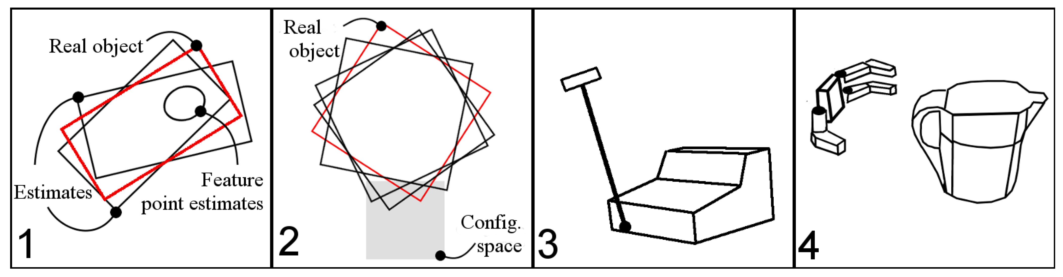
The aforementioned model is created to generalize from previous active-sensing works. Here, four examples conforming to the model are reported.

• An infrared sensing application where a plate is localized in 2DOFs [3].
• A force sensing application where a cube is localized in 3DOFs [9].
• A force sensing application where objects are localized in 6DOFs [10].
• A tactile sensing application where objects are localized in 3DOFs for grasping [4].

Graphically represented in Figure 1, they are summarized in Table 1 in terms of the six primitives.

Table 1. Prior examples of touch-based active sensing described with the six primitive concepts of the active sensing task model: configuration space, information space, object model, action space, inference scheme and action-selection scheme. POMDP, partially-observable Markov decision process.

Ex.	Ref.	Configuration Space	Information Space	Object Model	Action Space	Inference Scheme	Action Selection Scheme
1	[3]	2DOF pose of the target position to drill the hole	parametric posterior distribution	analytical model (rectangle)	infrared edge detection	extended Kalman filter	weighted covariance trace min.
2	[9]	3DOF pose of the object	discretized posterior distribution	polygonal mesh	depth-sampling with force sensor	grid method	not declared
3	[10]	6DOF pose of the object	discretized posterior distribution	polygonal mesh	depth-sampling with force sensor	scaling series	random selection
4	[4]	3DOF pose of the object	discretized posterior distribution	polygonal mesh	grasping and sweeping motions	histogram filter	POMDP with entropy min.

Table 1. Prior examples of touch-based active sensing described with the six primitive concepts of the active sensing task model: configuration space, information space, object model, action space, inference scheme and action-selection scheme. POMDP, partially-observable Markov decision process.

Ex.	Ref.	Configuration Space	Information Space	Object Model	Action Space	Inference Scheme	Action Selection Scheme
1	[3]	2DOF pose of the target position to drill the hole	parametric posterior distribution	analytical model (rectangle)	infrared edge detection	extended Kalman filter	weighted covariance trace min.
2	[9]	3DOF pose of the object	discretized posterior distribution	polygonal mesh	depth-sampling with force sensor	grid method	not declared
3	[10]	6DOF pose of the object	discretized posterior distribution	polygonal mesh	depth-sampling with force sensor	scaling series	random selection
4	[4]	3DOF pose of the object	discretized posterior distribution	polygonal mesh	grasping and sweeping motions	histogram filter	POMDP with entropy min.

Figure 1. Graphical illustration of literature examples of touch-based active sensing tasks conforming to the active sensing task model. Image numbers refer to Table 2. Images 1 to 4 are inspired from [3,9,10] and [4], respectively.

Figure 1. Graphical illustration of literature examples of touch-based active sensing tasks conforming to the active sensing task model. Image numbers refer to Table 2. Images 1 to 4 are inspired from [3,9,10] and [4], respectively.

4. DOF Decoupling Task Graph Model

4.1. Motivation

In Bayesian touch-based localization applications, the pose of an object is estimated by updating a belief over the configuration space, conditioned on the obtained measurements, that is an estimate of the position of the touch probe at the moment the ongoing motion is stopped because a pre-defined threshold on the force has been exceeded. Typically, such a probability distribution becomes multi-modal, due to the local nature of the available information, e.g., taking the form of a contact point and a normal vector. Under these conditions, optimal and computationally-efficient parametric Bayesian filtering models, such as the Kalman filter are not suited to capture the different modes of the probability distribution. Hence, non-parametric inference schemes relying on a discretization of the probability distribution must be adopted, such as grid-based methods [8,9] or particle filter [11,12]. Unfortunately, the computational complexity of these inference schemes linearly increases with that of the configuration space. Moreover, the complexity of the action selection is exponential in the DOFs of the configuration space and in the time horizon of the decision making. As a matter of fact, this sets an upper bound on the size of the problems that can be treated online, since the available resources are always finite. This curse of dimensionality is a strong driver to focus on the reduction of the complexity of active sensing tasks.

In a previous work, we studied human behavior during touch-based localization [13]. A test was carried out with 30 subjects asked to localize a solid object in a structured environment. They showed common behavioral patterns, such as dividing the task into a sequence of lower complexity problems, proving remarkable time efficiency in accomplishing the task compared to state-of-the-art robotics examples of similar applications. The key insight extracted from these experiments was that humans use “planar” motions (that is, only needing a two-dimensional configuration space) as long as they have not yet touched the object; then they switch to a three-dimensional configuration space, in order to be able to represent the position and orientation in a plane, of the (“polygonal hull” of the) object they had touched before; and only after that position and orientation have been identified with “sufficient” accuracy, they start thinking in a six-dimensional configuration space, to find specific geometric features on the object, such as grooves or corners. Several times, the humans were driven by finding out whether one particular hypothesis of such a geometric feature indeed corresponded to the one they had in their mental model of the object; when that turned out not to be the case, they “backtracked” to the three- or even two-dimensional cases. While this overall “topological” strategy was surprisingly repetitive over all human participants, it was also clear that different people used very different policies in their decisions about which action to select next: some were “conservative”, and they double or triple checked their hypothesis before moving further; others were more “risk taking”, and went for “maximum likelihood” decisions based on the current estimate of the object’s location; while still others clearly preferred to do many motions, quickly, but each resulting in larger uncertainties on the new information about the object location than the more carefully-executed motions of the conservative group.

Inspired by this result, approaches were sought to also allow robots to divide a localization application into a series of subtask adapting the problem complexity at run time; the primitives that are available for this adaptation are: execution time, information gain per action, time to compute the next action and the choice of the configuration space over which the search is being conducted. A formal representation of these adaptation possibilities would allow the robot to reason itself about how to tackle tasks with higher initial uncertainty, performing the action selection online. In this work, “online” means that the reasoning about which action to execute does not take longer than the actual action execution itself. Indeed, if reasoning takes longer, it would make more sense to let the robot just execute random motions, which easily do better than not moving at all while computing how to move “best”.

4.2. Model Formulation: Task Graph and Policy

Backed by the results of the human experiment and building upon [14], it became clear that a more extended task representation formulation was required, to allow task programmers to explicitly represent a robot-localization application: (i) in a modular fashion; (ii) with each module specified in a configuration space of the “lowest possible” dimension; and (iii) using one of several possible action selection strategies. To this end, the task graph is added to the task model as a new modeling primitive, with the explicit purpose of representing the relationship that connects the just-mentioned pieces of information to a sequence of subtasks: each such subtask is defined (possibly recursively) as an active sensing module, with concrete instances for all of its six task model primitives and with a concrete choice of configuration space dimension and a concrete choice of reasoning strategy. This formal representation then contains all of the information to reduce, at run-time, the computational complexity of estimation and action-selection.

Task graph: an oriented graph representing a localization application in which each node corresponds to an active-sensing task defined in its specific configuration space and with a specific search strategy. The task graph allows us to encode the sequential order in which subtasks can be executed. Arcs encode transitions between subtasks, which are triggered by events, for instance: a sensor signal reaching some specified threshold, a change in the level of uncertainty or a human-specified occurrence.

Policy: a path through a task graph, connecting subtasks and transitions. Different policies may be defined in a task graph. For instance, this could be done further to an empirical observation, as proposed in the experimental section of this work, or by learning. In order to select a policy, graph-search techniques from the literature can be applied, e.g., random selection, breadth-first or depth-first. Hence, as proposed in [14], an active sensing localization task requires decision making at two different levels:

• to select a policy, i.e., the sequence of subtasks to execute;
• to select an action within each subtask.

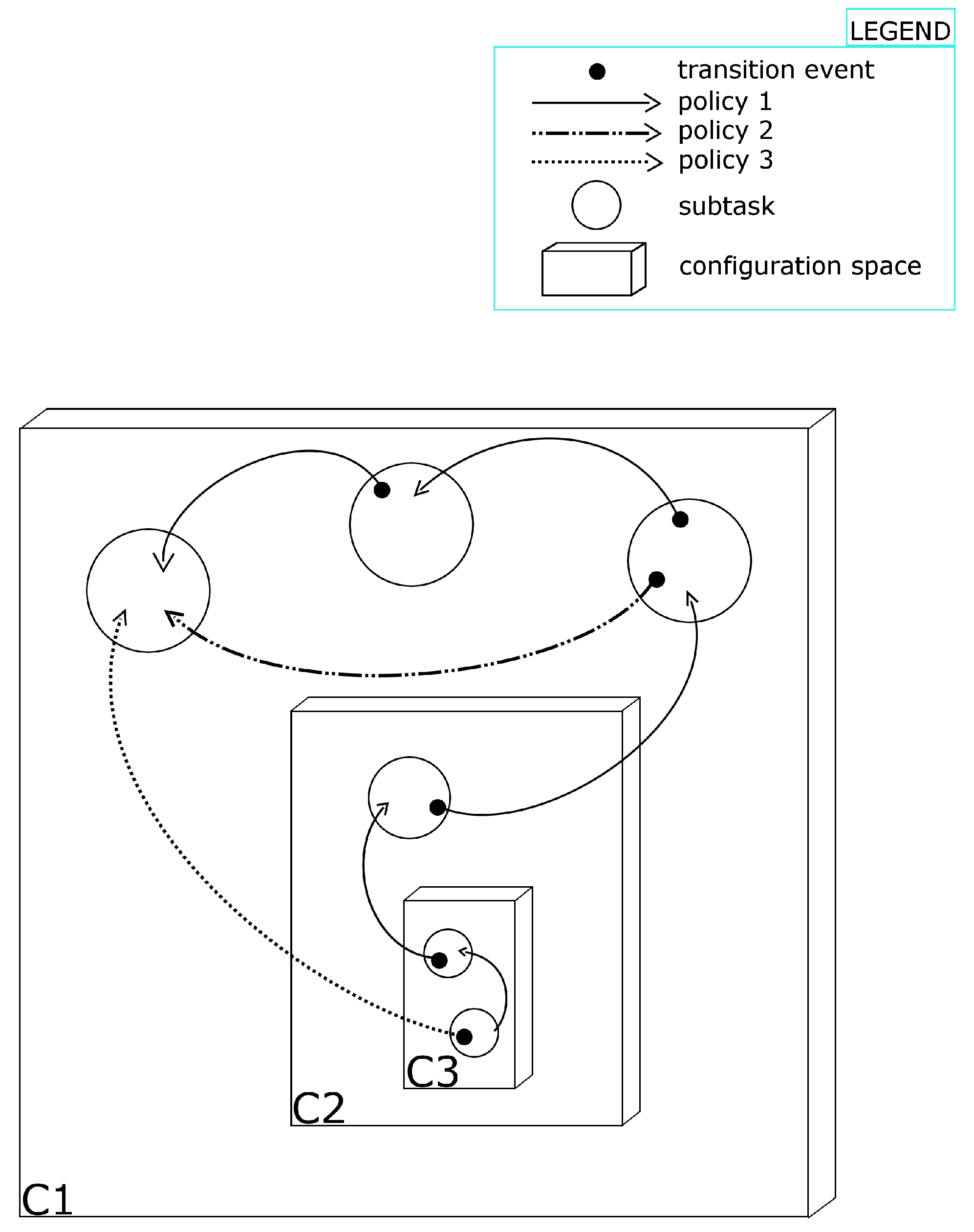
In general, the structure of the task graph is application dependent. For the sake of clarity, Figure 2 illustrates an example of a localization application described as a task graph with subtasks defined over three different configuration spaces: C1, C2 and C3. Three policies are available in the presented case, depicted with arrows of different patterns. Subtasks are represented as circles. It is important to note that several subtasks may be defined on the same configuration space, e.g., with different information space, object model, action space, inference and action-selection scheme. Transition events are depicted with a filled circle.

In this work, the DOF decoupling task graph model is exploited for touch-based active sensing applications. Policy generation and selection is done empirically, further to the human experiment observation. Building upon our previous work [15], the following section introduces a new action-selection algorithm, which is implemented on a practical case study in Section 7.3.

Figure 2. Example of task graph. Graphically, solid rectangles represent configuration spaces and circles represent subtasks. In this specific case, the task is defined over three configuration spaces, C1, C2 and C3, presenting three, one and two tasks, respectively. The localization is initialized in configuration space C3. Three policies are depicted with arrows of different patterns, each of them representing a possible way through the tasks defined over C1, C2 and C3.

Figure 2. Example of task graph. Graphically, solid rectangles represent configuration spaces and circles represent subtasks. In this specific case, the task is defined over three configuration spaces, C1, C2 and C3, presenting three, one and two tasks, respectively. The localization is initialized in configuration space C3. Three policies are depicted with arrows of different patterns, each of them representing a possible way through the tasks defined over C1, C2 and C3.

5. The act-reason Algorithm: Making Decisions over a Flexible Action Space

To the best of the authors’ knowledge, previous works on active sensing made decisions about where to sense next, maximizing some reward function choosing from a pre-defined action space composed of a set of sensing motions either specified by a human demonstrator or automatically generated off-line [4,5,8]. This resulted in an implicit choice on the complexity of the action space, hence also increasing the complexity of the action selection. In practice, this often caused the robot to devote a significant percentage of the running time to reasoning instead of acting.

5.1. Motivation

In the framework of the active sensing task model, there is the need to make the choice on the complexity of the action space explicit, thus allowing the robot to adjust the action-selection complexity at run time. With respect to the state-of-the-art, we introduce a new action-selection scheme named act-reason, which allows the robot to find a solution to the problem of where to sense next, constraining the time $t_{alloc}$ spent for the next action, including reasoning and motion execution. Therefore, the complexity of the action space depends on $t_{alloc}$ and the time required to reason about each action. In act-reason, $t_{alloc}$ is a design parameter that sets the robot behavior from info-gathering (increasing $t_{alloc}$) to motion-oriented (reducing $t_{alloc}$). In particular, this makes the action space flexible, so the complexity of the decision making can vary at run time.

5.2. Algorithm

Previous related works [5,8,16,17] tackled the problem of choosing the next best action $a^{*}$ by first generating a complete set of candidate actions $\left\{a\right\}$, then selecting the one that maximizes some specified reward function $r(.)$:

$$a^{*}=\text{arg}\underset{a}{max}E\left[r\right(a\left)\right]$$

(2)

Often, r corresponds to the information gain [3,7,14] or some task-oriented metric, such as the probability of grasping success, as proposed in [18]. However, the act-reason algorithm is independent of the chosen reward function, so it may apply to a generic robot task. For each sensing action a, the proposed scheme assumes the robot to be able to:

• generate the associated motion;
• evaluate the expected reward;
• estimate the execution time $t_{exec}$;
• estimate the evaluation time $t_{eval}$.

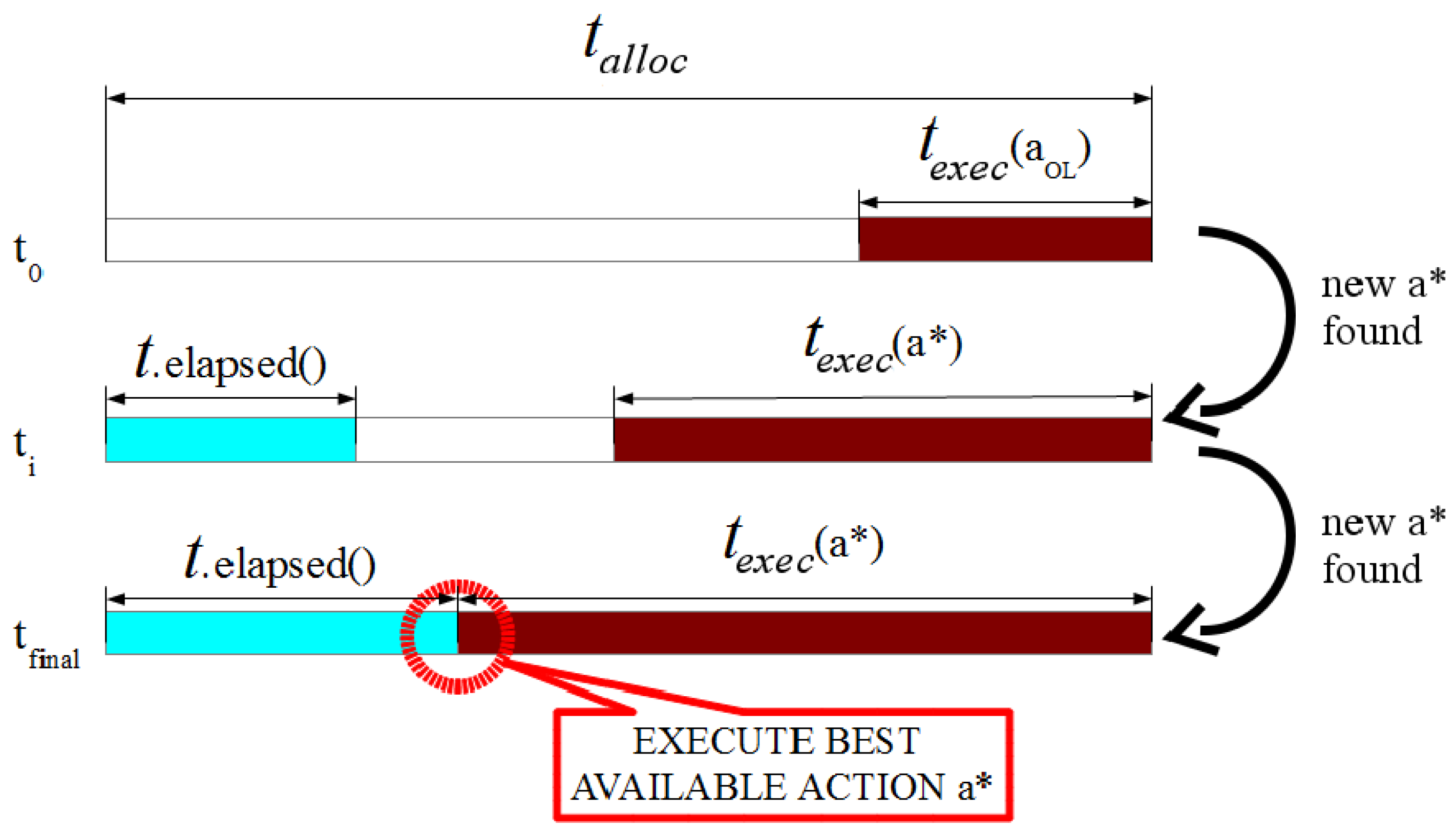
Intuitively, the action space is continuously sampled to estimate the expected reward that can be achieved within a preset total allocated time $t_{alloc}$. At each time step, the current best solution $a^{*}$ is stored. The $t_{alloc}$ parameter bounds the time spent to evaluate and execute the next action. Figure 3 graphically represents the action selection at different time steps: the starting time $t_0$, a generic instant $t_i$ and $t_{final}$ when $a^{*}$ is executed. In the illustrated case, an open-loop action is available, so $a^{*}$ is initialized to $a_{OL}$. As time passes, $a^{*}$ is updated, until $t.$elapsed() intersects $t_{exec}\left(a^{*}\right)$, and the current best action is executed.

The act-reason algorithm is presented in pseudo-code in Algorithm 1. Each time the robot needs to make a decision, the best solution $a^{*}$ is initialized to “stay still”, unless an open-loop action is available, e.g., a user-defined action (Lines 2–8). Then, the timer starts (Line 9). While the execution time of the current best solution is smaller than the available time ($t_{alloc}-t.\text{elapsed()}$), candidate actions are generated and evaluated, updating the best solution if the expected reward is greater than the current one (Lines 16–18). As the available time intercepts the estimated execution time of the current best solution, the reasoning is over, and $a^{*}$ is performed. The condition at Line 14 ensures that the next candidate to evaluate respects the time constraint.

A practical implementation of the act-reason algorithm is presented in Section 7.3, where $t_{alloc}$ is configured to minimize the execution time during a touch-based localization task.

Algorithm 1 Action selection with act-reason.

1: set $t_{alloc}$

2: if $a_{OL}$ is available then

3:  $a^{*}=a_{OL}$

4:  $E\left[r^{*}\right]=E\left[r\left(a_{OL}\right)\right]$

5: else

6:  $a^{*}=$ “stay still”

7:  $E\left[r^{*}\right]=0$

8: end if

9: t.start()

10: $i=0$

11: while $t_{exec}\left(a^{*}\right)<t_{alloc}-t$.elapsed() do

12:  $i:=i+1$

13:  $a_i=$ generateCandidateAction()

14:  if $t_{exec}\left(a_i\right)+t_{eval}\left(a_i\right)<t_{alloc}-t.$elapsed() then

15:   compute $E\left[r\left(a_i\right)\right]$

16:   if $E\left[r\left(a_i\right)\right]>E\left[r\left(a^{*}\right)\right]$ then

17:    $a^{*}=a_i$

18:   end if

19:  end if

20: end while

21: if $a^{*}==$ “stay still” then

22:  $t_{alloc}:=2t_{alloc}$

23:  go back to line 2 execute

24: end if

25: execute $a^{*}$

Figure 3. Action-selection time line with act-reason decision making. New candidate actions are generated and evaluated until the available time equals that required to execute the current best solution.

Figure 3. Action-selection time line with act-reason decision making. New candidate actions are generated and evaluated until the available time equals that required to execute the current best solution.

6. Robot Setup and Measurement Model

This work presents robotic applications of the DOF decoupling task graph model to touch-based localization. Specifically, the robot has to estimate the pose $\mathbf{x}$ of an object modeled as a polygonal mesh composed of faces $\left\{f_i\right\}$ and their associated normal vectors $\left\{n_i\right\}$. A single $<f_i,n_i>$ tuple will be referred to as patch. The pose of the object is represented by the state vector x, which collects its position and roll-pitch-yaw orientation with respect to the robot frame of reference R. In a Bayesian framework, the information on the pose of the object is encoded in the joint probability distribution over x conditioned on the measurement z: $P\left(\mathbf{x}\right|z)$. This section describes the robot set up and the measurement models adopted.

6.1. Contact Detection Model

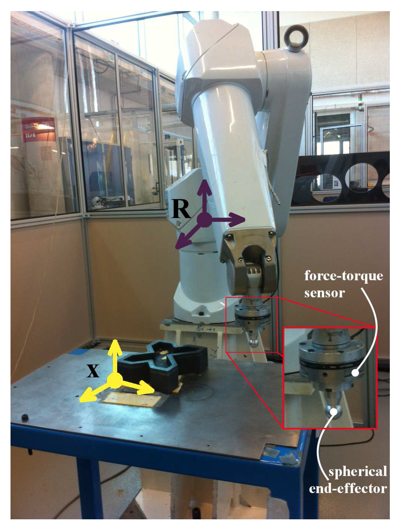
The robot is equipped with a spherical end-effector coupled with a force-torque sensor (as shown in Figure 4), and it acquires information about x both when moving in free space and when in contact with the object, assuming that interactions only take place with its end-effector. In this context, an action consists of the end-effector following a trajectory τ, sweeping a volume $\psi \left(\tau \right)$. Concretely, τ is a collection of end-effector frames $\left\{\varphi \right\}$ used as a requirement for the robot controller. When a contact is detected, the motion is stopped with the end-effector in frame ${\varphi }_c$. In case of no-contact, the whole trajectory is executed with the end-effector reaching pose ${\varphi }_{end}$. The sensory apparatus is comprised of a force-torque sensor used as a collision detector setting an amplitude threshold on the measured forces. Specifically, it detects whether the end-effector is in contact with the object (C) or is moving in free space ($NC$):

$$z_{CD}=\left\{\begin{array}{c}C\text{,}\text{if}\text{the}\text{resultant}\text{force}\text{reaches}\text{the}\text{threshold}\hfill \\ NC\text{,}\text{otherwise}\hfill \end{array}\right.$$

(3)

Figure 4. Robot setup used for the experimental test. The pose of the object $\mathbf{x}$ is represented with respect to the robot reference frame R.

Figure 4. Robot setup used for the experimental test. The pose of the object $\mathbf{x}$ is represented with respect to the robot reference frame R.

When the end-effector touches the object, the point of contact $z_P$ and the normal vector $z_n$ of the touched point can be estimated following the procedure described by Kitagaki et al. [19], under the assumption of frictionless contact. We will refer to this touch measurement as $z_{touch}$:

$$z_{touch}=\{z_P,z_n\}$$

(4)

As in [4], in order to define the observation models, we consider two possible cases: (i) the robot reaches the end of the trajectory; and (ii) the robot makes contact with the object stopping in ${\varphi }_c$.

6.2. The Robot Reaches the End of the Trajectory without Contact

Intuitively, we need to model the probability that the robot executes the trajectory τ without touching the object in a given pose x. The Boolean function $\xi (\mathbf{x},\tau )$ is used to indicate whether $\psi \left(\tau \right)$ intersects the volume of the object, Equation (5):

$$\xi (\mathbf{x},\tau )=\left\{\begin{array}{c}1\text{,}\text{if}\psi \left(\tau \right)\text{intersects}\text{the}\text{object}\text{in}\text{pose}\mathbf{\text{x}}\hfill \\ 0\text{,}\text{otherwise}\hfill \end{array}\right.$$

(5)

Building upon [8], the contact-detection measurement is modeled as in Equation (6). α and β represent the false-negative and false-positive error rates for the contact detection.

$$P\left(z_{CD}\right|\mathbf{x},\tau )=\left\{\begin{array}{c}P(z_{CD}=NC|\xi (\mathbf{x},\tau )=1)=\alpha \hfill \\ P(z_{CD}=C|\xi (\mathbf{x},\tau )=1)=1-\alpha \hfill \\ P(z_{CD}=C|\xi (\mathbf{x},\tau )=0)=\beta \hfill \\ P(z_{CD}=NC|\xi (\mathbf{x},\tau )=0)=1-\beta .\hfill \end{array}\right.$$

(6)

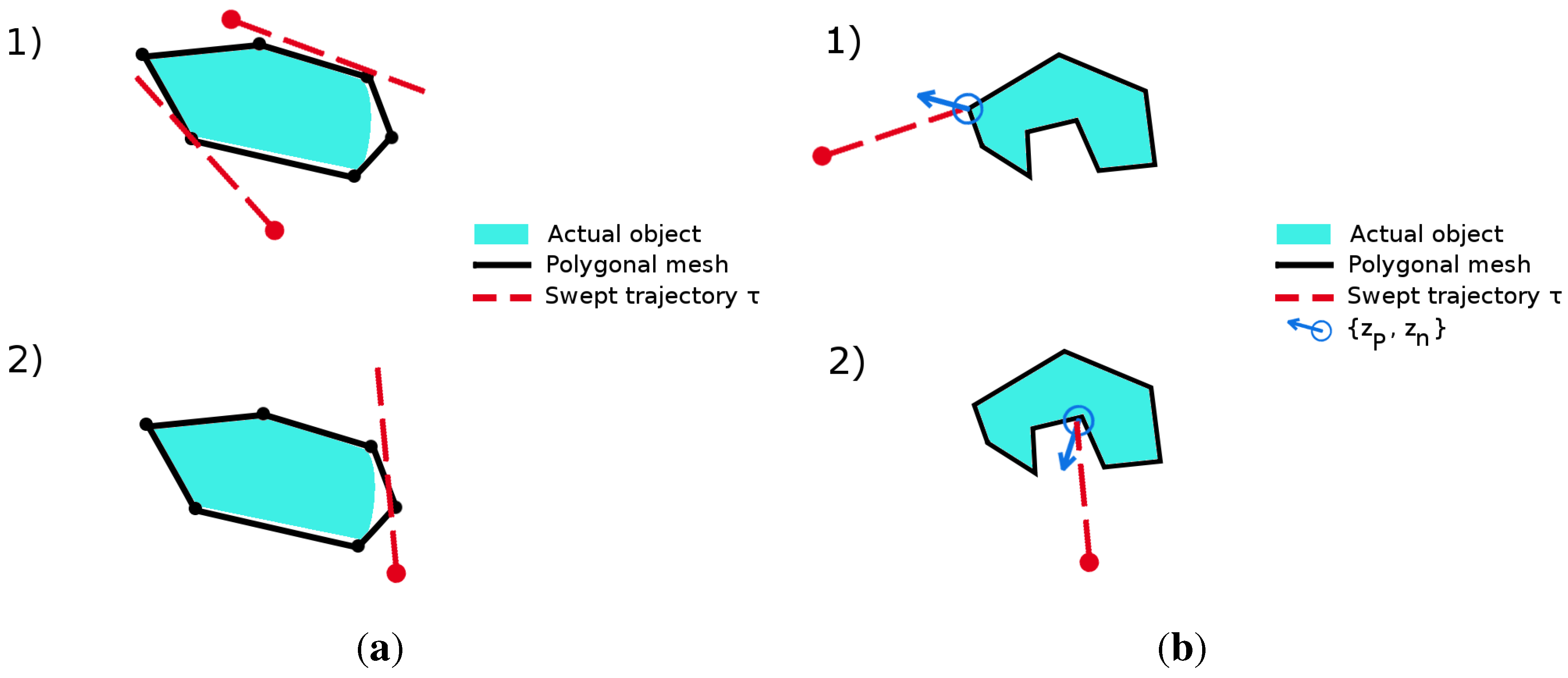
The false-negative error rate α corresponds to the probability of not measuring contact when the sweep intersects the volume occupied by the object. This coefficient captures two main sources of uncertainty. Firstly, when the robot measures $z_{CD}=NC$, it might actually be in contact with the object, but in some configuration that prevents the force-torque signals from reaching the thresholds. Figure 5a1 illustrates an example of such a false-negative measurement situation when the limited stiffness of the controller and the low surface friction allow the robot to contact the object and slide over it without exceeding the thresholds. Secondly, α also captures the uncertainty related to the mismatch between the object model and the actual object, which may cause the robot to intersect the polygonal mesh without measuring any real contact. An example of the latter situation is depicted in Figure 5a2. In general, α is a function of the intersection between $\psi \left(\tau \right)$ and the volume occupied by the object in pose $\mathbf{x}$. In this work, this computation is simplified assuming α as a function of the penetration length l, which is the intersection of the nominal trajectory τ and the volume of the object.

Figure 5. False-negative contact situations (a); and biased contact measurement situations (b). (a) Possible false-negative contact-detection situation: (1) the end effector touches the object sliding over it without exceeding the force threshold; (2) the end effector sweeps through the geometric model without touching the real object. (b) Examples of the contact state possibly leading to an inaccurate measurement: the end effector touches a vertex (Case 1) or a corner (Case 2). The measured normal does not correspond to any of the adjacent faces of on the object.

Figure 5. False-negative contact situations (a); and biased contact measurement situations (b). (a) Possible false-negative contact-detection situation: (1) the end effector touches the object sliding over it without exceeding the force threshold; (2) the end effector sweeps through the geometric model without touching the real object. (b) Examples of the contact state possibly leading to an inaccurate measurement: the end effector touches a vertex (Case 1) or a corner (Case 2). The measured normal does not correspond to any of the adjacent faces of on the object.

The false-positive error rate β encodes the probability of measuring contact when the sweep does not intersect the object volume. The threshold to detect contact is set on the resultant force and is parametrized with respect to the maximum standard deviation error among those of the force signals. This guarantees a lower false contact error rate than other thresholding policies, e.g., ellipsoidal or parallelepiped. In addition, we make the assumption of modeling the object with a polygonal mesh that is external or at most coincident to the nominal geometry. Moreover, the limited speed of the robot makes inertial effects minimal. Under these conditions, the probability of measuring a false contact is negligible. This corresponds to assuming $\beta \approx 0$.

In practice, the likelihood function $P_{free}$ corresponding to a sweep without contact along τ and object pose x is expressed in Equation (7).

$$P_{free}(\mathbf{x},\tau )=P\left(NC\right|\xi (\mathbf{x},\tau ))$$

(7)

6.3. The Robot Makes Contact with the Object

Let us name ${\tau }_c$ the trajectory executed by the robot following τ up to pose ${\varphi }_c$ on which the contact is detected. The measurement model expresses the probability of observing no-contact along ${\tau }_c$, plus a contact in ${\varphi }_c$ with touch measurement $z_{touch}$:

$$P_{contact}(\mathbf{x},\tau )=P_{free}(\mathbf{x},{\tau }_c)P(z_{CD},z_{touch}|\mathbf{x},{\varphi }_c)$$

(8)

$P_{free}(\mathbf{x},{\tau }_c)$ can be calculated as in Equation (7). By the definition of conditional probability:

$$P(z_{CD},z_{touch}|\mathbf{x},{\varphi }_c)=P\left(z_{touch}\right|\mathbf{x},{\varphi }_c,z_{CD})P\left(z_{CD}\right|\mathbf{x},{\varphi }_c)$$

(9)

where $P\left(z_{CD}\right|\mathbf{x},{\varphi }_c)$ is calculated as in Equation (6). Formally, ${\varphi }_c$ corresponds to the single-frame trajectory at which a contact is detected. However, in case of non-perfect proprio-perception or measurement capabilities, this may correspond to a portion of the trajectory instead of a single frame.

The touch measurement $z_{touch}$ is comprised of both contact point $z_P$ and normal vector $z_n$. This is observed only when the robot actually touches the object, i.e., when $z_{CD}=C$:

$$P\left(z_{touch}\right|\mathbf{x},{\varphi }_c,z_{CD})=P(z_P,z_n|\mathbf{x},{\varphi }_c,z_{CD}=C)$$

(10)

In the case of non-spherical end-effector, in [20], techniques have been presented to estimate the geometric parameters of the contacted surface through continuous force-controlled compliant motions. Since our final application case is comprised of harsh scenarios presenting rough and possibly soiled surfaces, we may not assume the robot to be capable of performing compliant motions in such environments. Instead, actions with the spherical pin used as a depth-probing finger are here considered as motion primitives. Unfortunately, with such actions, it is possible to experience contact states leading to inaccurate measurements, e.g., when the pin touches the object over a vertex, an edge or a corner. In this case, the normal vector measurement is significantly biased with respect to the nominal vector of the adjacent faces, as depicted in Figure 5b.

As in [4,8,10], we adopt the simplifying approximation of supposing both measurements $z_P$ and $z_n$ independent if conditioned on $\mathbf{x},{\varphi }_c$ and $z_{CD}$. Therefore, the joint measurement probability can be expressed as in Equation (11).

$$P(z_P,z_n|\mathbf{x},{\varphi }_c,z_{CD})=P\left(z_P\right|\mathbf{x},{\varphi }_c,z_{CD})P\left(z_n\right|\mathbf{x},{\varphi }_c,z_{CD})$$

(11)

With the object modeled as a polygonal mesh $\{f_i,n_i\}$ in pose x and with the robot in pose ${\varphi }_c$, one can express the likelihood functions encoding the probability of each patch $<f_i,n_i>$ to cause $z_P$ and $z_n$ as in Equations (12) and (13). Specifically, the uncertainty on $z_{touch}$ is due to the noise acting on the six channels of the force-torque signal, to vertex or edge contact interaction (as depicted in Figure 5b) and surface imperfections. Such noise is assumed to be Gaussian for both $z_P$ and $z_n$.

$$P\left(z_P\right|f_i,{\varphi }_c,C)=\frac{1}{\sqrt{2\pi }{\sigma }_p}exp\left[-\frac{1}{2}\frac{dist{(z_P,f_i)}^2}{{\sigma }_p^2}\right]$$

(12)

and:

$$P\left(z_n\right|n_i,{\varphi }_c,C)=\frac{1}{\sqrt{2\pi }{\sigma }_n}exp\left[-\frac{1}{2}\frac{\left|\right|z_n-n_i{\left|\right|}^2}{{\sigma }_n^2}\right]$$

(13)

The operator $dist(z_P,f_i)$ returns the distance between a measured point $z_P$ and a face $f_i$ of the polygonal mesh, whereas $\left|\right|z_n-n_i\left|\right|$ is the norm of the difference between the measured normal vector and the patch normal vector. After experimental tests, the Gaussian assumption for Equations (12) and (13) proves legitimate to model the uncertainty due to the measurement system and the non-perfect surface of the object. Yet, this model does not effectively capture the edge and vertex contact states depicted in Figure 5b. This limitation results in some estimation outliers, as further explained in Section 7.1.

The likelihood functions in Equations (12) and (13) are written with respect to a single $<f_i,n_i>$ patch, while the object model is composed by a whole mesh. Since it is necessary to express the likelihood functions with respect to the whole mesh in pose x, a maximum-likelihood approach can then be applied: the patch $<f^{*},n^{*}>$ that maximizes the product of both the contact and normal likelihoods is the one used to calculate the likelihood, as in Equation (14).

$$<f^{*},n^{*}>=\text{arg}\underset{<f_i,n_i>}{max}\left(P\left(z_P\right|f_i,{\varphi }_c,C)P\left(z_n\right|n_i,{\varphi }_c,C)\right)$$

(14)

This association strategy is also referred to as hard assign [21], and it implies an over-estimation of the likelihood function for the pose x:

$$P\left(z_{touch}\right|\mathbf{x},{\varphi }_c)=P\left(z_P\right|f^{*},{\varphi }_c,C)P\left(z_n\right|n^{*},{\varphi }_c,C)$$

(15)

Alternatively, one may also follow a soft assign approach, considering the likelihood of the pose as a linear combination of the likelihood of its faces. Since computing Equations (12) and (13) prove to be computationally expensive, the latter option is neither adopted in the literature nor in this work.

Nevertheless, even using Equation (14), computing contact and normal probabilities may become cumbersome when using large meshes. Instead, as already proposed by [4], one may select the face that only maximizes $P\left(z_P\right|f_i,{\varphi }_c,C)$, as in Equation (16).

$$f^{*}=\text{arg}\underset{f_i}{max}\left(P\left(z_P\right|f_i,{\varphi }_c,C)\right)$$

(16)

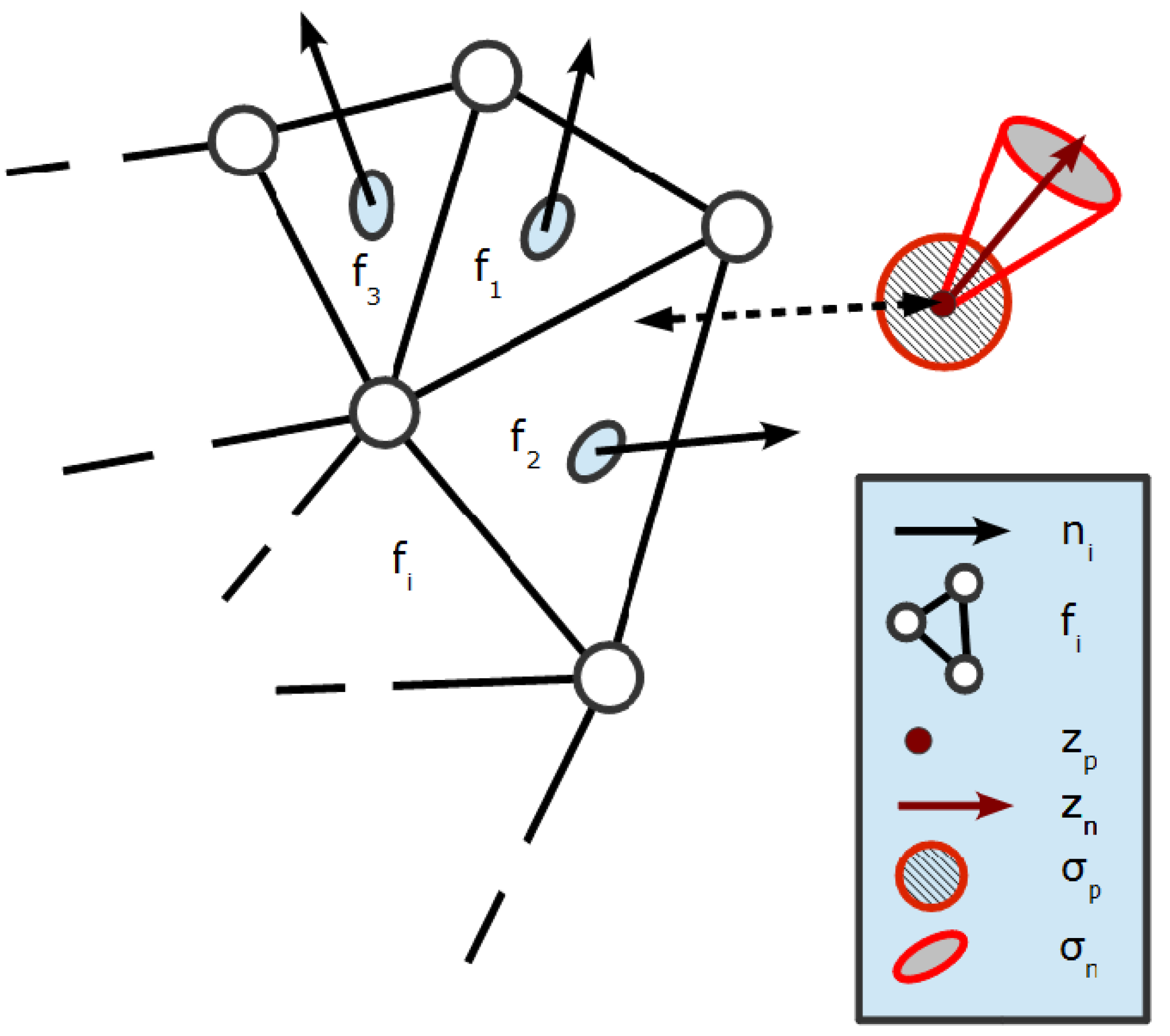
This allows the estimator to speed up the calculation, since Equation (13) is computed only once, but it prevents the model from considering the normal likelihood when selecting the face. However, this simplification may be considered legitimate when ${\sigma }_p\ll {\sigma }_n$ (for instance, with a difference of orders of magnitude). For the sake of clarity, Figure 6 illustrates an example of the object mesh with a measured contact and normal vector affected by Gaussian noise. Being the closest to the contact point, face $f_2$ is selected to represent the pose of the object in terms of the likelihood function Equation (17):

$$P\left(z_{touch}\right|\mathbf{x},{\varphi }_c,C)=P\left(z_P\right|f_2,{\varphi }_c,C)P\left(z_n\right|n_2,{\varphi }_c,C).$$

(17)

Figure 6. Polygonal mesh representing the object as a set of face-normal tuples $<f_i,n_i>$. The contact and normal vector are modeled as affected by Gaussian noise, represented by a sphere of radius ${\sigma }_p$ and a cone of radius ${\sigma }_n$, respectively.

Figure 6. Polygonal mesh representing the object as a set of face-normal tuples $<f_i,n_i>$. The contact and normal vector are modeled as affected by Gaussian noise, represented by a sphere of radius ${\sigma }_p$ and a cone of radius ${\sigma }_n$, respectively.

6.4. Inference Scheme

The state ${\mathbf{x}}_t\in X$ represents the pose of the object with respect to the robot frame of reference at time t. Its evolution over time is described as a hidden Markov model, i.e., a dynamical stochastic system where ${\mathbf{x}}_t$ depends only on the previous state ${\mathbf{x}}_{t-1}$. This derives from the Markov assumption of state completeness, i.e., no variable prior to ${\mathbf{x}}_{t-1}$ may influence the evolution of the future states. The state-measurement model can then be summarized as:

$$\begin{array}{ccc}& & {\mathbf{x}}_t=g\left({\mathbf{x}}_{t-1}\right)+{\delta }_t\hfill \end{array}$$

(18)

$$\begin{array}{ccc}& & z_t=m\left({\mathbf{x}}_t\right)+{ϵ}_t\hfill \end{array}$$

(19)

where $g(.)$ and $m(.)$ are the transition model and measurement functions and ${\delta }_t$ and ${ϵ}_t$ are transition and measurement noises. In a Bayesian context, the state is inferred updating a posterior distribution over the configuration space accounting for the measurement $z_t$, which is modeled as a set of independent random variables $z_t$ drawn from the conditional probability distribution $P\left(z_t\right|{\mathbf{x}}_t)$, also referred to as likelihood. The motion model is encoded by the transition probability $P\left({\mathbf{x}}_t\right|{\mathbf{x}}_{t-1})$. Our estimation objective is to infer the posterior probability over the state given the available measurement $P\left({\mathbf{x}}_t\right|z_{0:t})$. In this work, the notation proposed in [22] is taken as a reference to represent the state transition and update. Specifically, $b\overline{e}l\left({\mathbf{x}}_t\right)$ and $bel\left({\mathbf{x}}_t\right)$ are used to denote these two conditional probabilities, as in Equations (20) and (21).

$$b\overline{e}l\left(x_t\right)=P\left({\mathbf{x}}_t\right|z_{0:t-1})$$

(20)

$$bel\left(x_t\right)=P\left({\mathbf{x}}_t\right|z_{0:t})$$

(21)

A Bayesian filter requires two steps to build the posterior probability, a prediction and an update. During prediction, the belief is calculated as in Equation (22), projecting the state from time $t-1$ to time t using the transition model.

$$b\overline{e}l\left(x_t\right)={\int }_{{\mathbf{x}}_{t-1}}P\left({\mathbf{x}}_t\right|{\mathbf{x}}_{t-1})b\overline{e}l\left({\mathbf{x}}_{t-1}\right)d{\mathbf{x}}_{t-1}$$

(22)

During the update, the posterior probability is updated multiplying the belief $\overline{bel}$ by the measurement likelihood and the normalization factor η. Intuitively, this corresponds to a correction of the model-based prediction based on measured data:

$$bel\left(x_t\right)=\eta P\left(z_t\right|{\mathbf{x}}_t)b\overline{e}l\left({\mathbf{x}}_t\right)$$

(23)

In our application, the measurement likelihood $P\left(z_t\right|{\mathbf{x}}_t)$ is calculated as in Equations (7) and (8). In the case of motion without contact, the transition model is the identity matrix. In the case of contact, the transition model is a diagonal covariance matrix ${\Sigma }_{contact}$:

$${\Sigma }_{contact}={\sigma }_{contact}^{2}I$$

(24)

where ${\sigma }_{contact}$ is used to model the uncertainty on the object pose introduced by the contact. The normalization factor η is calculated as:

$$\eta =\frac{1}{{\int }_{{\mathbf{x}}_t}P\left(z_t\right|{\mathbf{x}}_t)\overline{bel}\left({\mathbf{x}}_t\right)d{\mathbf{x}}_t}$$

(25)

and assures that the posterior probability sums up to one. Since we may not assume the posterior distribution over the state to be unimodal and the measurement is not linear, Equations (12) and (13), a particle filter algorithm is adopted. Its implementation is presented in pseudocode in Algorithm 2, with χ representing the particle set. ${\chi }_0$ is initialized with samples drawn uniformly over the configuration space. Every time an action is completed, the algorithm is run. In the case of contact, the weights are calculated according to Equation (8). In the case of the trajectory finishing without contact, the weight is updated according to Equation (7).

Algorithm 2 Object localization with particle filter.
1: ${\chi }_t=\left[\right]$
2: for $i=1:N$ do
3:  $\text{sample}{x}_t^{\left[i\right]}\sim P\left(x_t\right|x_{t-1}^{\left[i\right]})$	⊳ Draw particle from transition model
4:  if contact then	⊳ update contact weight
5:   $w_t^{\left[i\right]}=P_{free}(x_t^{\left[i\right]},{\tau }_c)P(C,z_{touch}|x_t^{\left[i\right]},{\varphi }_c)$
6:  else	⊳ Update no-contact weight
7:   $w_t^{\left[i\right]}=P_{free}(x_t^{\left[i\right]},\tau )$
8:  end if
9:  $\text{add}{x}_t^{\left[i\right]}\text{to}{\overline{\chi }}_t$
10: end for
11: for $i=1:N$ do
12:  $\text{draw}\text{index}\text{m}\text{from}\{x_t^{\left[i\right]},w_t^{\left[i\right]}\}$	⊳ Resampling with replacement
13:  $\text{add}{x}_t^{\left[m\right]}\text{to}{\chi }_t$
14: end for
15: for $i=1:N$ do
16:  ${\tilde{w}}_t^{\left[i\right]}=\frac{w_t^{\left[i\right]}}{{\sum }_0^N{w}_t^{\left[i\right]}}$	⊳ Normalization
17: end for

7. Experimental Results

Experimental results are presented in the context of touch-based active sensing using the robot setup described in the previous section. Focusing on industrial relevance, this work improves the state-of-the-art:

• localizing objects up to industrial geometric complexity;
• localizing an object with high initial uncertainty, keeping the estimation problem tractable using the DOF decoupling task graph model;
• speeding up an object localization task using the act-reason algorithm setting the allocated time as a function of the current uncertainty.

7.1. Localization of Objects of Increasing Complexity

To the best of our knowledge, literature examples presented case studies with polygonal meshes up to about 100 faces [8,10]. Here, we contribute to the state-of-the-art localizing objects up to industrial complexity. The application is specified with a task graph with as a single task:

• configuration space: the pose of the object $\mathbf{x}=\{x,y,{\theta }_z\}$ defined with respect to the robot frame of reference. Initial uncertainty: (0.1 m, 0.1 m, 1 rad).
• Information space: $P\left(\mathbf{x}\right|z)$.
• Object model: polygonal mesh.
• Action space: user-defined actions aiming at touching the largest faces of the object in the best-estimate pose. Sensing: contact detection and touch measurement.
• Inference scheme: particle filter.
• Action-selection scheme: random selection.

Table 2 presents the objects used in the experiment: the solid rectangle (${\text{obj}}_{\text{SR}}$), the v-block (${\text{obj}}_{\text{VB}}$), the cylinder-box (${\text{obj}}_{\text{CB}}$) and the ergonomy test mock-up (${\text{obj}}_{\text{ET}}$). Together with their properties, mesh and action space, the table shows the obtained localization results. In this test, ${\sigma }_P=0.005$ m and ${\sigma }_n=0.1$.

The following protocol was followed for each run:

• Actions were repeated until 80% of the probability mass on the target position (indicated in red in Table 2) was concentrated around a 5-mm radius, which is consistent with the tolerance allowed in typical robot operations, e.g., for grasping and manipulation applications. The probability threshold was chosen to be the same as in [4].
• Once the 80% confidence threshold was reached, a peg-in-hole sequence aiming at the target on the object was performed recording the final position of the spherical end-effector.
• The end-effector was manually positioned on the target spot and the end-effector position recorded.

The considered ground truth about the position of the target was biased by the uncertainty related to human vision. After empirical observation, this can be estimated on the order of 2 mm. Even if biased, this may be considered as a genuine mean to evaluate the localization accuracy. Table 2 presents the localization results in terms of final $\{x,y\}$ target position error with respect to the observed ground truth (Loc.error). The mean $\overline{e}$ and the standard deviation of the error norm ${\sigma }_e$ are also reported.

Overall, the tests carried out on the ${\text{obj}}_{\text{VB}}$ present the best accuracy in terms of mean error norm, even though an outlier was recorded due to a vertex contact, as shown in Figure 5a. Unsurprisingly, tests on ${\text{obj}}_{\text{ET}}$ present the highest mean and standard deviation error, yet with most of the bias concentrated along the x axis. This is likely due to a non-negligible misalignment between the polygonal mesh and the actual geometry of the object, which experienced plastic displacement due to heavy usage previous to this test.

Table 2. Summary of the object localization tests. For each studied object, the table reports geometric and dynamic characteristics, action space, localization error, mean error norm $\overline{e}$ and error norm standard deviation ${\sigma }_e$.

Object	Obj ${}_{\text{SR}}$	Obj ${}_{\text{VB}}$	Obj ${}_{\text{CB}}$	Obj ${}_{\text{ET}}$
Size (m)	0.15 × 0.15 × 0.1	0.175 × 0.15 × 0.05	0.35 × 0.125 × 0.08	0.44 × 0.14 × 0.14
Vertices	8	96	191	915
Faces	12	188	376	1,877
Weight (kg)	1.2	3	5.4	10.5
Model
Actions
Loc. error
$\overline{e}$ (m)	0.005	0.0043	0.0053	0.0073
${\sigma }_e$ (m)	0.0025	0.0034	0.0052	0.0048

Table 2. Summary of the object localization tests. For each studied object, the table reports geometric and dynamic characteristics, action space, localization error, mean error norm $\overline{e}$ and error norm standard deviation ${\sigma }_e$.

Object	Obj ${}_{\text{SR}}$	Obj ${}_{\text{VB}}$	Obj ${}_{\text{CB}}$	Obj ${}_{\text{ET}}$
Size (m)	0.15 × 0.15 × 0.1	0.175 × 0.15 × 0.05	0.35 × 0.125 × 0.08	0.44 × 0.14 × 0.14
Vertices	8	96	191	915
Faces	12	188	376	1,877
Weight (kg)	1.2	3	5.4	10.5
Model
Actions
Loc. error
$\overline{e}$ (m)	0.005	0.0043	0.0053	0.0073
${\sigma }_e$ (m)	0.0025	0.0034	0.0052	0.0048

7.2. Touch-Based Localization with High Initial Uncertainty

Localising an object in 3DOFs over a table with a tolerance of 5 mm and initial uncertainty (0.4 m, 0.4 m, 2π) may become computationally expensive and prevent online action-selection. Prior work examples of similar tasks [4,8,12,14] suffered from this curse of dimensionality, requiring several minutes to perform the task. In this section, we show how the complexity of the task can be reduced adopting an empirical task graph derived from the human experiment presented in [13] and applying it to the localization of obj${}_{\text{VB}}$. 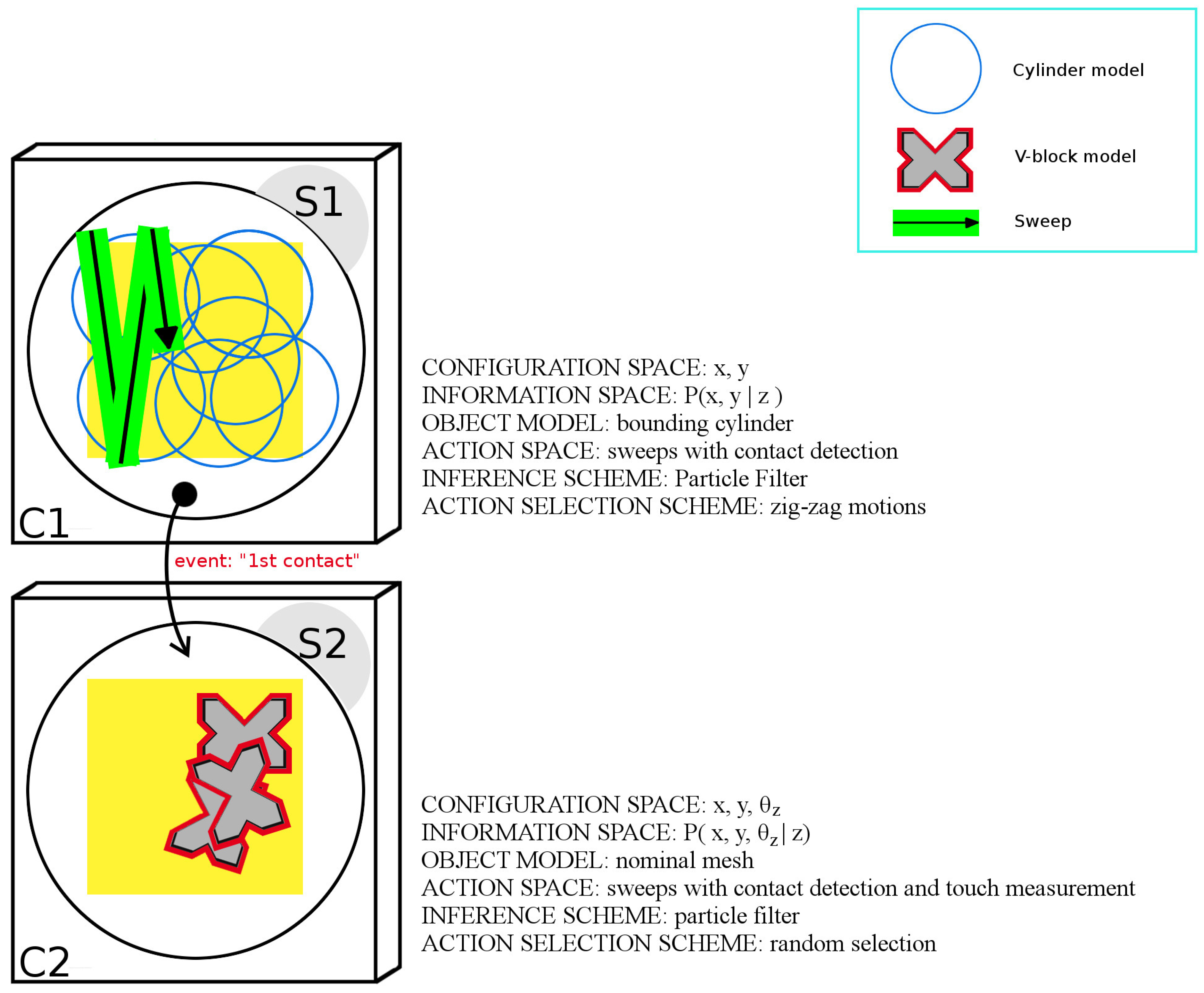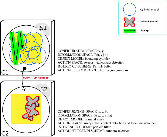Specifically, the application is divided into two subtasks, S1 and S2, as detailed below and illustrated in Figure 7.

• Subtask S1:

  –

  configuration space C1: $\{x,y\}$ position of the object with respect to the robot.

  –

  information space: P(x|z).

  –

  object model: polygonal mesh of the bounding cylinder of obj${}_{\text{VB}}$.

  –

  action space: sweep with contact detection.

  –

  inference scheme: particle filter.

  –

  action-selection scheme: zig-zag motions parametrized with respect to the table dimensions.

• Subtask S2:

  –

  configuration space C2: $\{x,y,{\theta }_z\}$ pose of the object with respect to the robot.

  –

  information space: posterior distribution over the object configuration space given the contact measurement.

  –

  object model: nominal polygonal mesh of obj${}_{\text{VB}}$.

  –

  action space: sweeps with contact detection and touch measurements.

  –

  inference scheme:particle filter.

  –

  action-selection scheme: random actions aiming at the four faces of the object in its best-estimate configuration.

Figure 7. Task graph derived from the human experiment in [13]. The application is divided into an initial 2DOF subtask (S1) defined over configuration space C1 and a second subtask (S2) defined over configuration space C2.

Figure 7. Task graph derived from the human experiment in [13]. The application is divided into an initial 2DOF subtask (S1) defined over configuration space C1 and a second subtask (S2) defined over configuration space C2.

S1 is aimed at reducing the uncertainty on x and y applying a zig-zag action-selection strategy that spans the table surface in a breadth-first fashion. The object is represented as the cylinder that bounds obj${}_{\text{VB}}$ and has radius ρ. Inference is performed through a particle filter. The action space is comprised of sweeps with contact detection. S2 is aimed at finely estimating the pose of the object, which is represented with its nominal mesh. Inference is performed with a particle filter. The action space is comprised of sweeps with contact detection and touch measurement aiming at 12 different faces of obj${}_{\text{VB}}$ (see Table 2). 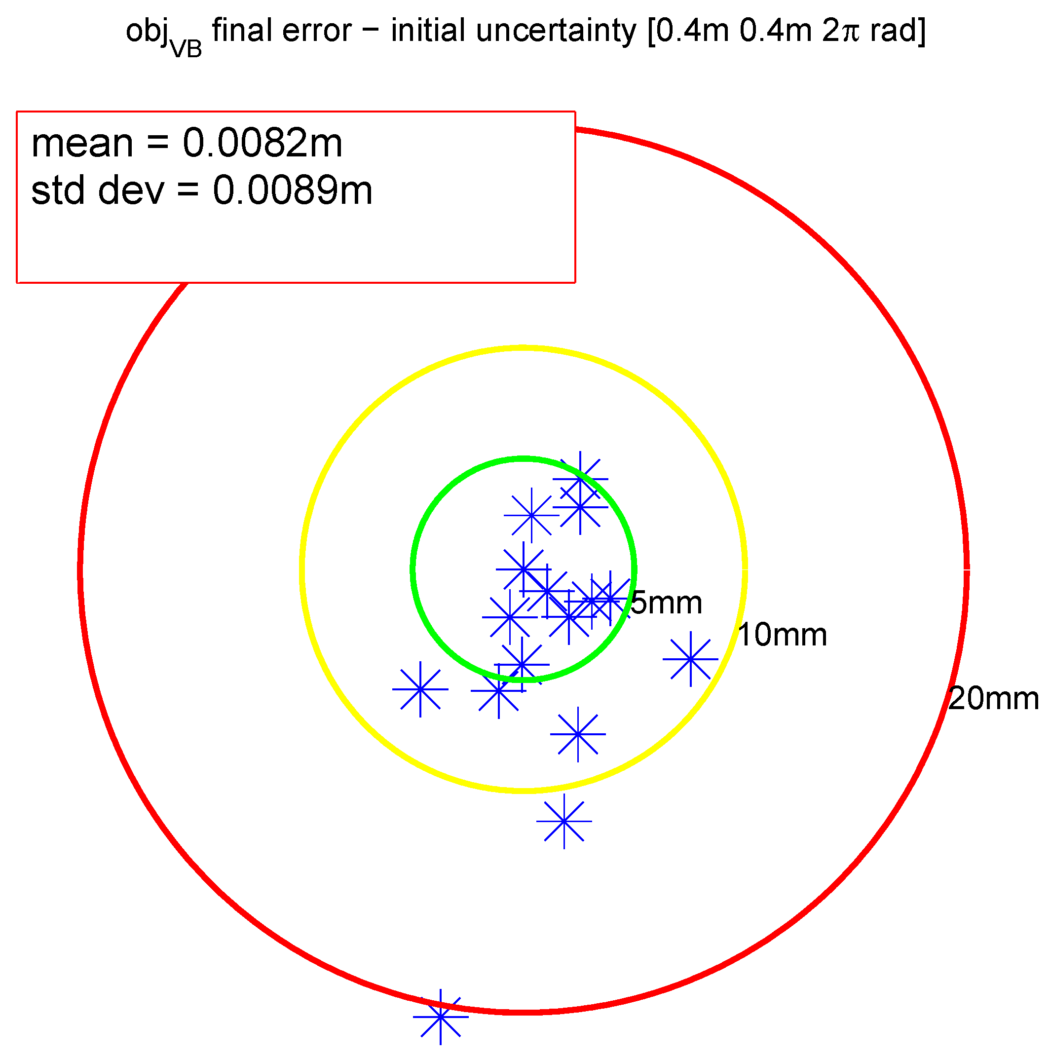To capture geometric imperfections, α was set to 5 mm. The same protocol presented in SubSection 7.1 was followed. Fifteen trials were carried out with the object located in a random pose on top of the table. In all cases, task execution took less than 120 s, and the final error position of the end-effector is reported in Figure 8.

Figure 8. Peg-in-hole error during v-block localization with DOF decoupling with (0.4 m, 0.4 m, 2π) initial uncertainty.

Figure 8. Peg-in-hole error during v-block localization with DOF decoupling with (0.4 m, 0.4 m, 2π) initial uncertainty.

7.3. Reducing Task Execution Time with the act-reason Algorithm

In the context of touch-based localization, different action-selection schemes have been adopted in the literature, including random selection [12], entropy minimization [4] and Kullback–Leibler divergence [8]. However, in these examples, actions were selected from a predefined action space, with a significant impact of computation over task execution time. Here, the focus is on time efficiency, and we present a concrete example of how the act-reason algorithm can be adopted to improve it with respect to random selection and entropy minimization. According to Equation (2), the reward corresponds to the difference of the entropy H of the prior distribution at time t and the entropy of the posterior distribution after the action a is executed:

$$r\left(a\right)=H\left(P\left({\mathbf{x}}_t\right)\right)-H\left(P\left({\mathbf{x}}_{t+1}\right)\right|a).$$

(26)

In this work, the particle filter formulation of entropy proposed by [5] is adopted.

Formally, the studied localization application of obj${}_{\text{VB}}$ is represented by the six following primitives of the active sensing task model.

• Configuration space: the pose of the object $\mathbf{x}=\{x,y,{\theta }_z\}$ defined with respect to the robot frame of reference. Initial uncertainty: (0.1 m 0.1 m 1 rad).
• Information space: $P\left(\mathbf{x}\right|z)$.
• Object model: polygonal mesh of obj${}_{\text{VB}}$.
• Action space: user-defined actions aiming at touching the largest faces of the object in its best-estimate pose. Sensing: contact detection and touch measurements.
• Inference scheme: particle filter.
• Action-selection scheme:

  • random selection
  • entropy minimization
  • act-reason with entropy minimization.

In this context, task progress can be evaluated through the current uncertainty on the pose of the object. During preliminary tests, random selection was compared to entropy minimization. The better performance of a random action-selection was observed, especially at the beginning of the localization, while an entropy minimization strategy generated more informative actions, yet taking longer for their evaluation. Intuitively, at the beginning of the localization, very little information is available, and any contact is likely to reduce the uncertainty significantly. At this stage, one would wish to follow a random selection to obtain fast contacts. Instead, when more information is available, spending more time reasoning to find the best action through entropy minimization tends to pay off.

In order to exploit both the benefits of an initial random strategy and the informative actions obtained with an entropy-based selection, we adopt the act-reason algorithm to vary the allocated time to reason and execute depending on the current uncertainty, as in Equation (27). Specifically, we set the allocated time $t_{alloc}$ to vary between the average time required by a random action ${\widehat{t}}_{rand}$ and that of a full-resolution entropy minimization ${\widehat{t}}_{ent}$, considering both computation and execution. For the sake of simplicity, this variation is set linear in the progress metric Π:

$$t_{alloc}={\widehat{t}}_{rand}+\Pi ({\widehat{t}}_{ent}-{\widehat{t}}_{rand}).$$

(27)

In our implementation, Π is defined as the ratio between the current probability mass within the 5-mm tolerance and the desired value to call the localization done.

$$\Pi =\frac{P(\mathbf{x}\in tol)}{P{(\mathbf{x}\in tol)}_{final}}.$$

(28)

Intuitively, this corresponds to adjusting the robot behavior from fully random when the uncertainty is high, to fully info-gathering when the uncertainty is low and more informative actions improve convergence.

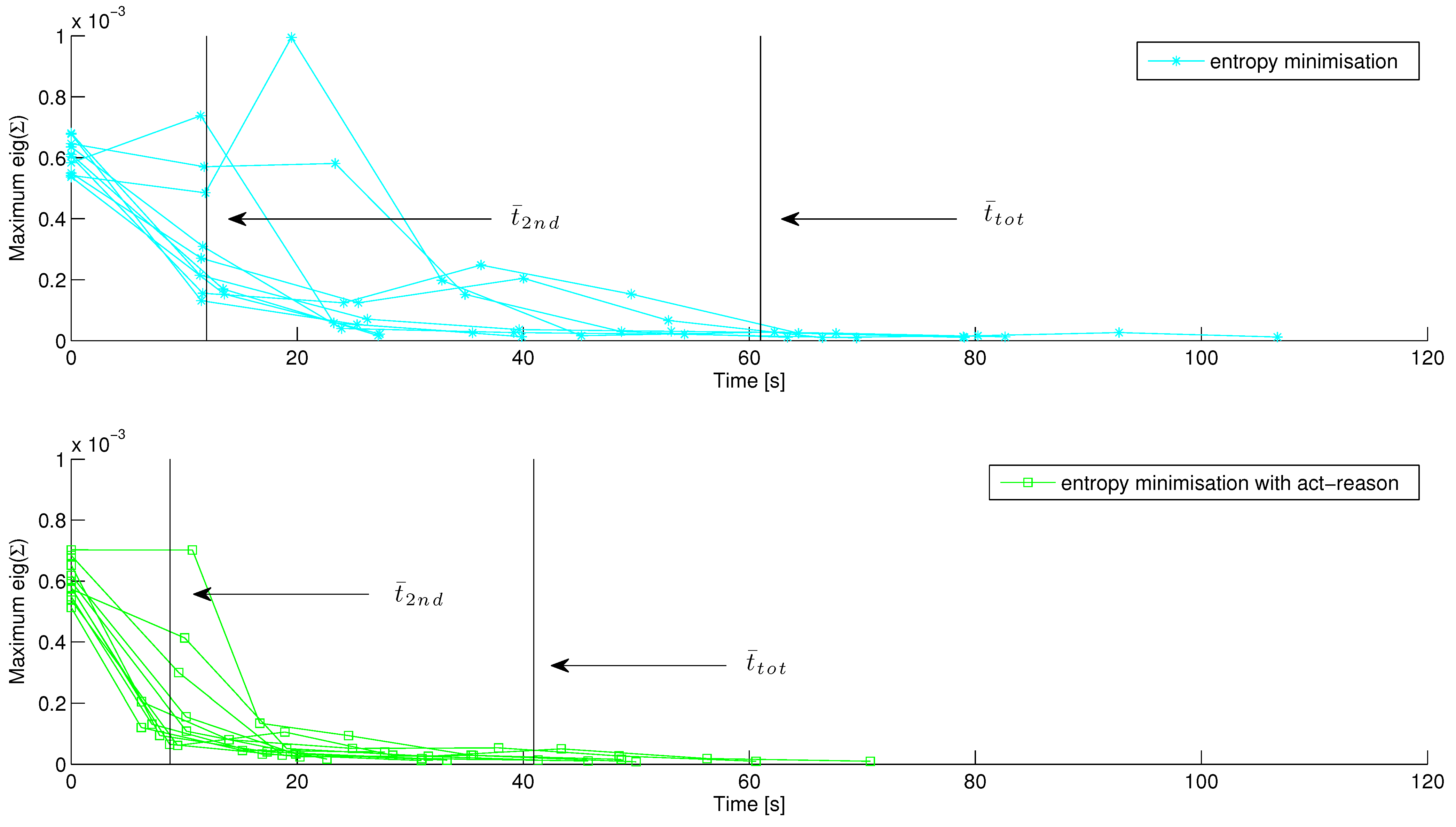
Figure 9 presents the results in terms of information gain vs. time during a v-block localization with initial uncertainty of (0.1 m, 0.1 m, 1 rad). Applying the act-reason algorithm to vary $t_{alloc}$ as in Equation (27), a faster second contact and a lower execution time is recorded. In Table 3, the average task-execution time ${\overline{t}}_{tot}$ and the average time to second contact ${\overline{t}}_{2nd}$ are reported. With act-reason, task-execution time is reduced by 52% with respect to entropy minimization and by 35% with respect to random selection.

Table 3. V-block localization with initial uncertainty (0.1 m, 0.1 m, 1 rad): comparison of task-execution time and time to second contact with act-reason, entropy minimization and random selection.

	Act-Reason	H Min.	Random
${\overline{t}}_{tot}$ (s)	40.1	61.0	54.0
${\overline{t}}_{\text{2nd}}$ (s)	8.7	12.0	8.4

Table 3. V-block localization with initial uncertainty (0.1 m, 0.1 m, 1 rad): comparison of task-execution time and time to second contact with act-reason, entropy minimization and random selection.

	Act-Reason	H Min.	Random
${\overline{t}}_{tot}$ (s)	40.1	61.0	54.0
${\overline{t}}_{\text{2nd}}$ (s)	8.7	12.0	8.4

Figure 9. V-block localization with initial uncertainty (0.1 m, 0.1 m, 1 rad). Progress vs. time with fixed action space (cyan) and variable action space using the act-reason algorithm (green).

Figure 9. V-block localization with initial uncertainty (0.1 m, 0.1 m, 1 rad). Progress vs. time with fixed action space (cyan) and variable action space using the act-reason algorithm (green).

8. Conclusions

Active sensing has been almost exclusively an academic research interest, with strong emphasis on search algorithms, with proofs of concept demonstrations on rather simple objects and without paying much attention to the overall time to realize the task. However, with sensor-based robots becoming more commonplace in industrial practice, there is a drive towards more performant active sensing task selection, on objects with the geometric complexity of industrial applications. Hence, there is a large demand to reduce the time it takes to compute, execute and process the active sensing actions.

The contribution of this paper that is expected to have the biggest impact on such a time reduction is the insight that the state-of-the-art until now has been using the implicit assumption that an active sensing task that needs to localize geometric features on objects in the six-dimensional configuration space of those features’ position and orientation should also do all of its computations in that same six-dimensional configuration space. However, our extensive observations of humans performing active sensing showed that they are very good at adapting the dimension of the search space to the amount of information that has already been found. The main gain in speed then comes from using only two- or three-dimensional motions to find the first contact with the object; after that, similar low-dimensional searches can be used, for example to scan a planar face of the object for the feature. Many different strategies are possible for how to choose such lower-dimensional searches, but the major observation is that humans only switch to the eventual six-dimensional search space towards the very end of the active sensing task.

The other contributions of this paper also have an impact on the desired reduction in the computation of active sensing actions, by suggesting a formal model of active sensing, in which all relevant aspects are represented separately, as well as the relationships between these aspects that a particular active sensing computation must take into account.

First, and generalizing from previous examples in the literature, a model-level representation of active sensing tasks has been presented. The novelty of the model is in the introduction of the task graph primitive, which allows one to divide a task into a sequence of subtasks defined over less complex configuration spaces than the default six-dimensional one of the objects’ position and orientation. In addition, the task graph also stores the choice of search strategies to be used in the corresponding subtask. The information that becomes available in this way provides online reasoners with more options to reduce the computational complexity, thus speeding up the localization task.

The act-reason algorithm has been formulated and implemented to solve the action-selection problem once the task graph is chosen. Specifically, it allows the robot to reason over a variable action space, explicitly trading off information gain, execution cost and computation time.

Experimental results on touch-based applications have contributed to the state-of-the-art: (i) localizing four objects of different complexity up to about ${10}^3$ vertices; (ii) localizing a solid object with high initial uncertainty without suffering from the curse of dimensionality thanks to the task graph structure; and (iii) improving the time efficiency of object localization using act-reason, setting the allocated time as a function of the current uncertainty.

9. Discussion and Future Work

Applying an empirical task graph observed during a human experiment, significant complexity reduction was achieved on a 3DOF force-based localization application. Enhancing these results by defining the task graph out of a constrained optimization would represent a remarkable extension of our findings. In this regard, the distributional clauses particle filter framework [23] might be adopted to encode topological relations between different objects, such as {inside, on top, beside}, in order to define the structure of the task graph from the CAD model of the environment.

The object model presented in Section 3.1 takes into account geometric properties. This information is sufficient to perform active sensing with probes, such as vision or force sensors. However, this model could be extended to take into account additional information, such as dynamic or thermic properties of the object, which can be exploited by other types of sensors.

An action space composed of more complex touch primitives (e.g., compliant motion for contour following) could exploit the edges and corners of the object to gather more information for the estimation.