
Leveraging Qualitative Reasoning to Learning Manipulation Tasks

Abstract
:1. Motivation
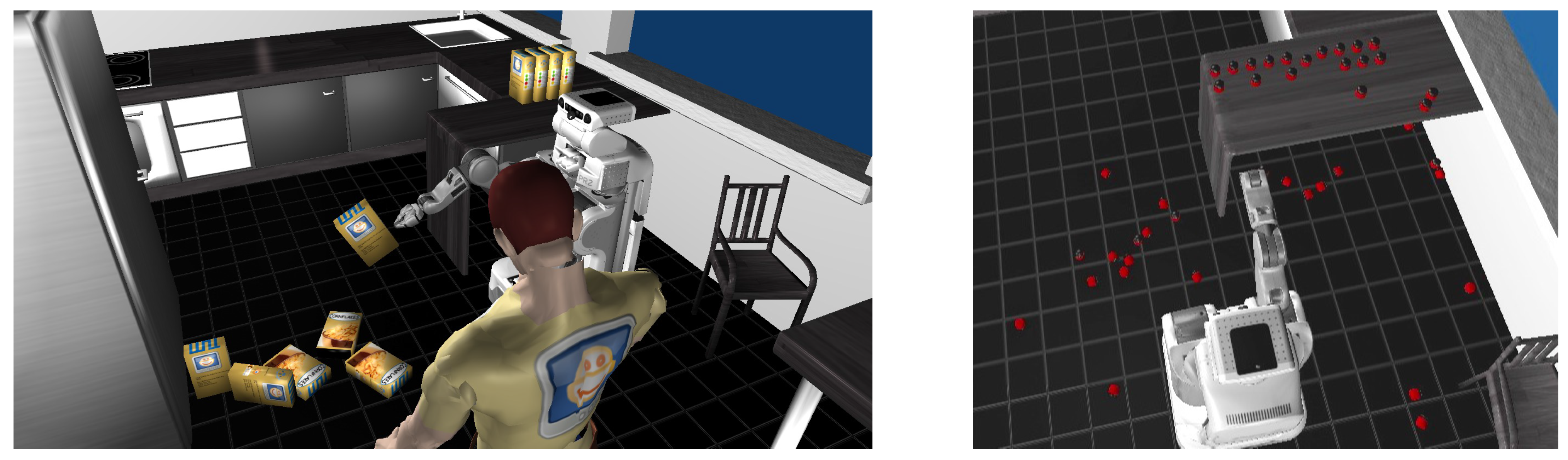
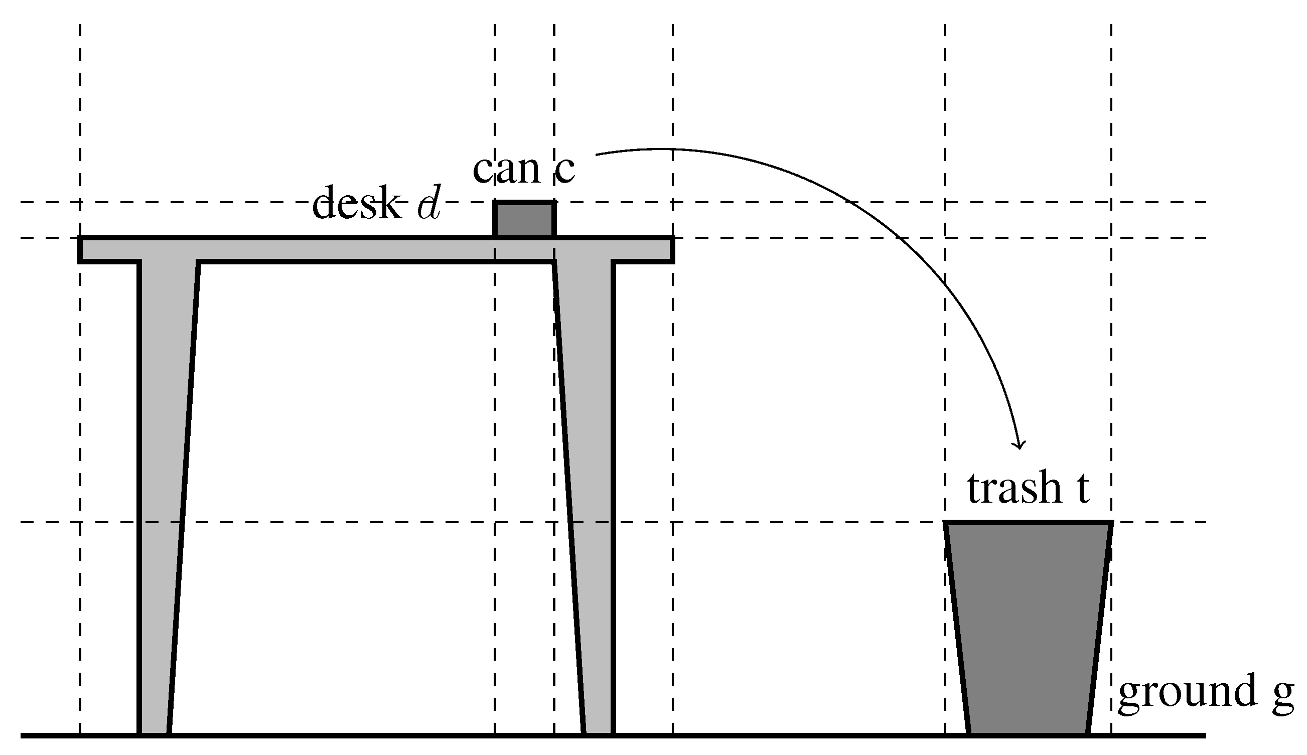
1.1. Scenario

1.2. Approach and Contribution

2. Qualitative Representation of Manipulation Tasks with Qualitative Spatial Logic (QSL)
2.1. Qualitative Representation of Space


2.2. Spatial Logic of Manipulation Tasks
2.2.1. Syntax and Semantics of Qualitative Spatial Logic (QSL)


| ∘ | next | holds in next world |
| ⋄ | eventually | |
| □ | always | |
| until | ϕ holds until ψ holds at some point in future | |
| release | ϕ released ψ, if ψ stops to hold at some future point, ϕ will hold, |
2.3. Reasoning with QSL
- Task specifications gain their expressivity from the rich set of spatial primitives that can be employed, not from the complex temporal interrelationships which makes model checking hard.
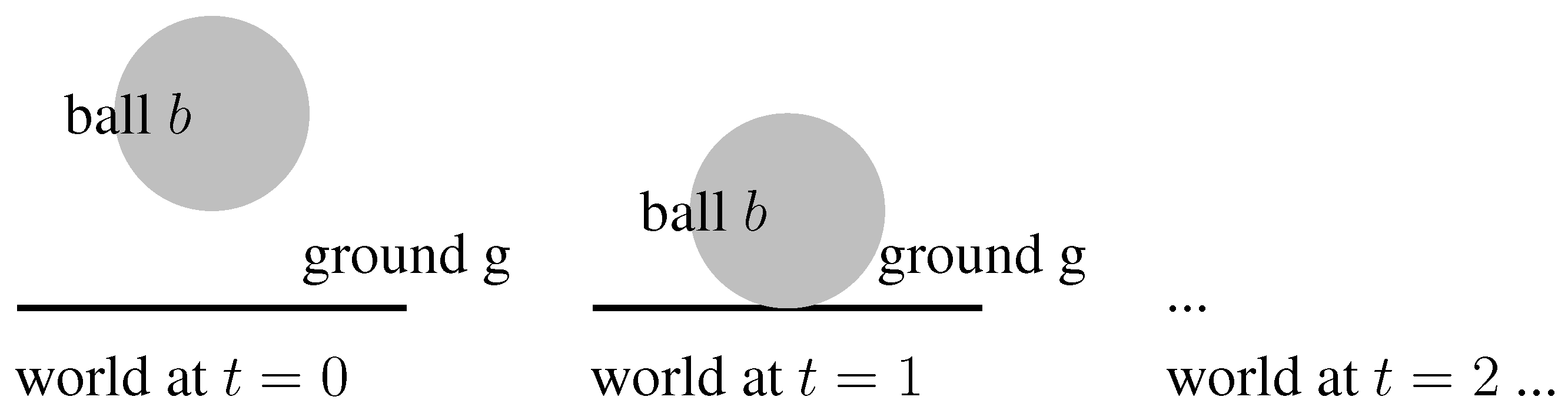
- Tasks are of short duration and models derived from observing the process are thus small. For example, throwing a ball takes few seconds only, which if observed at 100 Hz rate only leads to a few thousand worlds.

3. Qualitative Spatial Logic in Learning and Planning
3.1. Determining and Classifying Instances for Learning
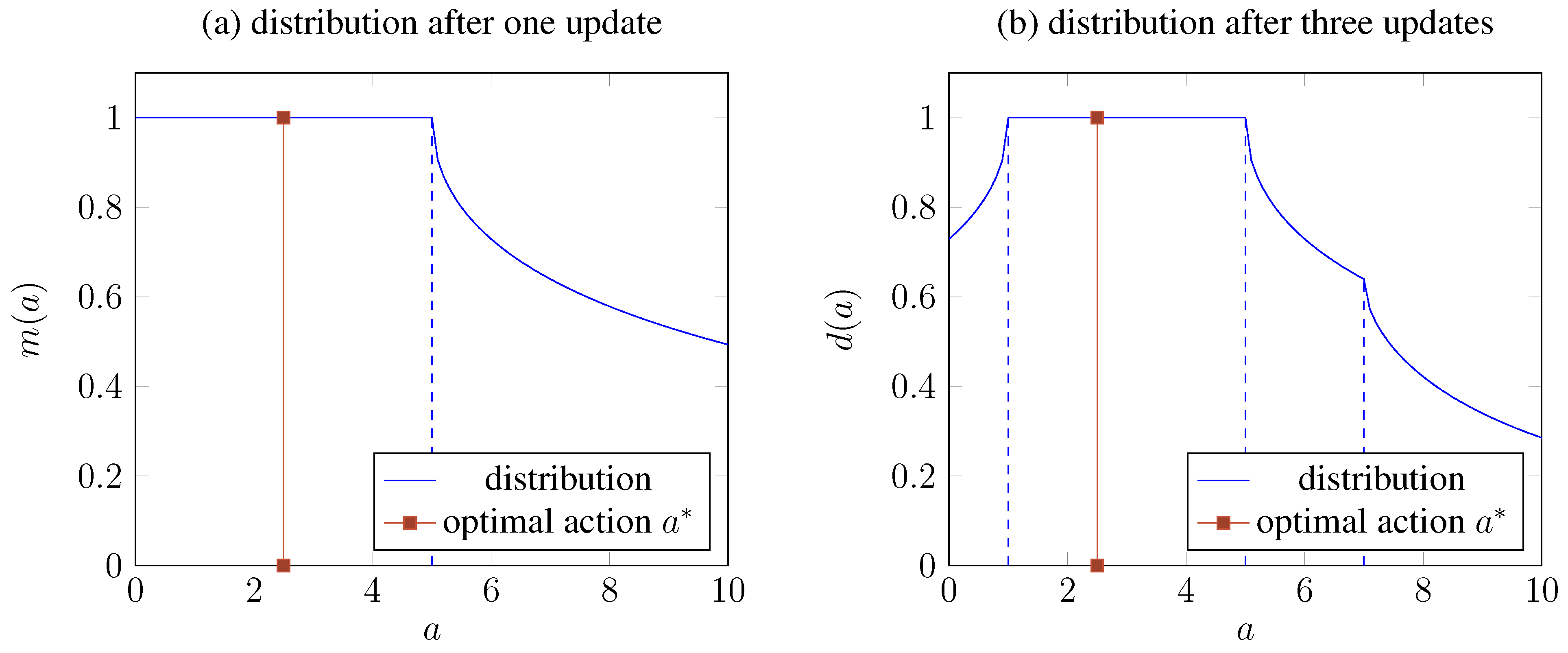
3.2. Enhancing Efficiency of Action Planning by Reasoning

4. Evaluation of QSL-based Reasoning for Planning
4.1. Experimental Setup
- height of release over ground between 0.5 m and 1.5 m
- vertical velocity between −1.0 m and 3.0 m/s
- horizontal velocity between 0.0 m and 3.0 m/s (negative values would be symmetrical)

4.2. Learning the Forward Model
| Noise in | Number of | Observed Distances | Learning Errors | ||
|---|---|---|---|---|---|
| Environment | Training Instances | Max | Min | MAE | RMSE |
| no noise | 924 | 0.0149 | 2.57376 | 0.0 | 0.0205 |
| no noise | 73 | 0.0594 | 1.88315 | 0.0 | 0.079 |
| noise | 924 | 0.1466 | 3.01778 | –0.32156 | 0.1939 |
| noise | 89 | 0.1943 | 2.8557 | –0.32156 | 0.258 |
4.3. QSL-Based Reasoning for Planning
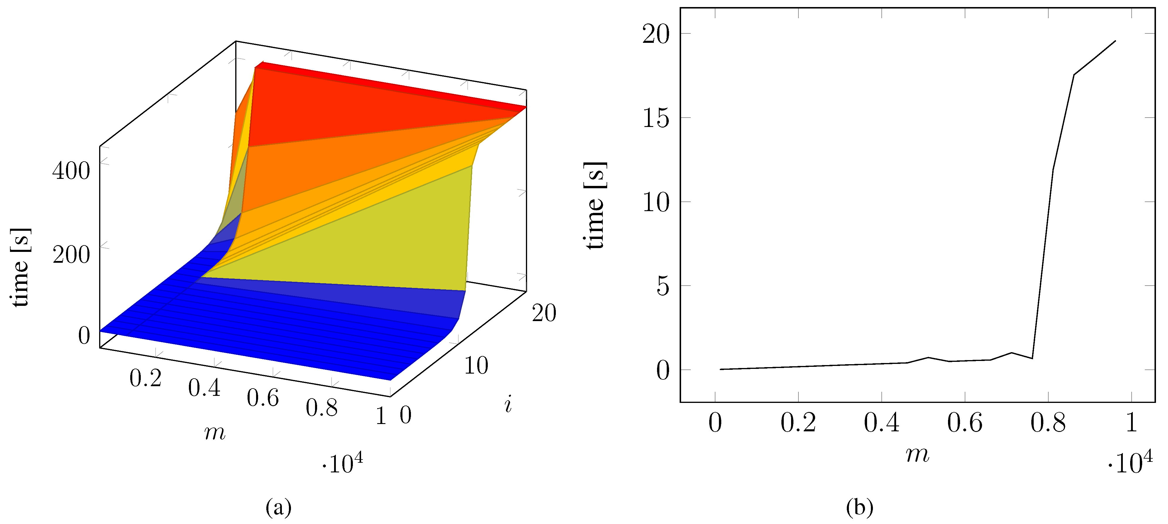
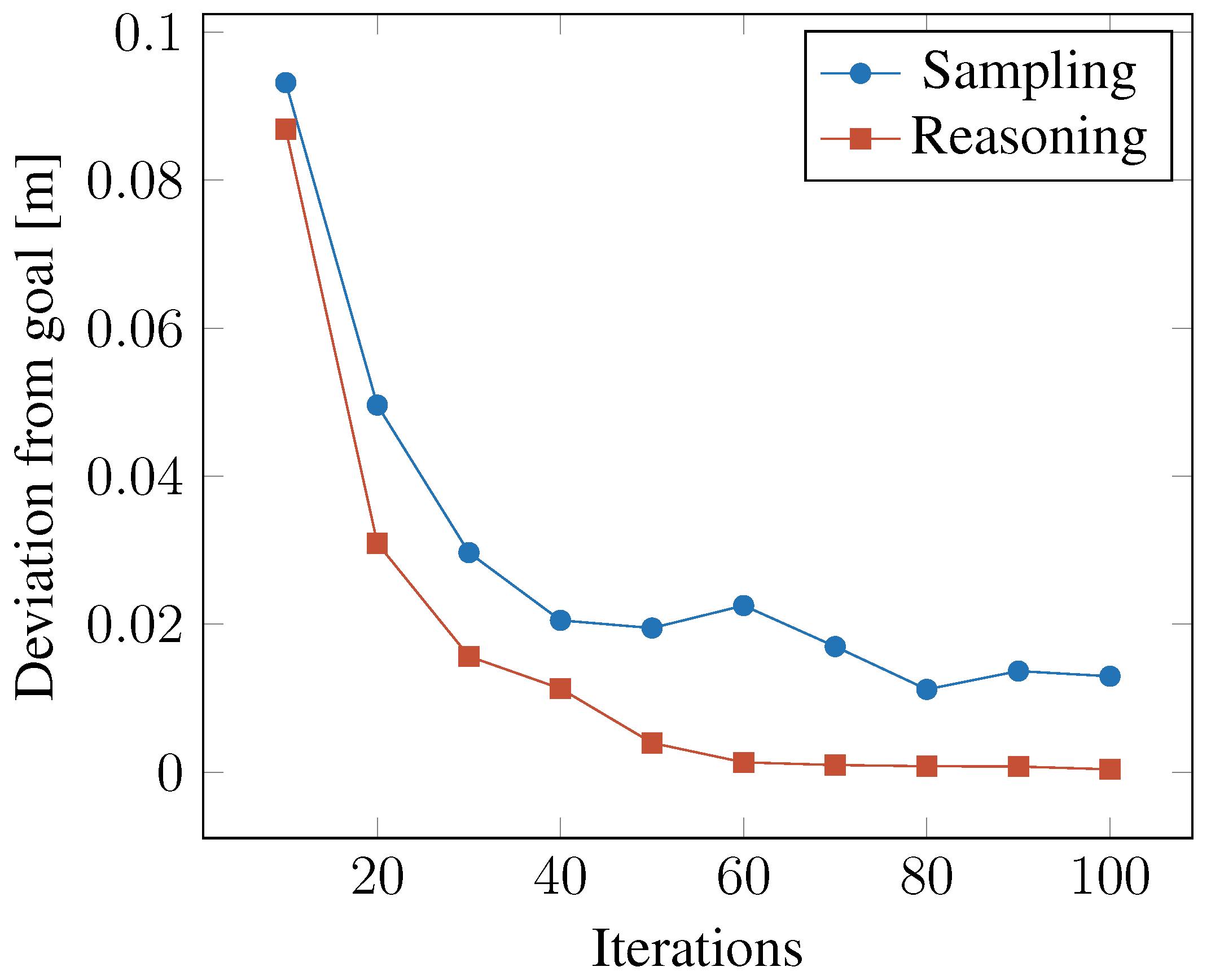
4.4. Determining the Iteration Cutoff

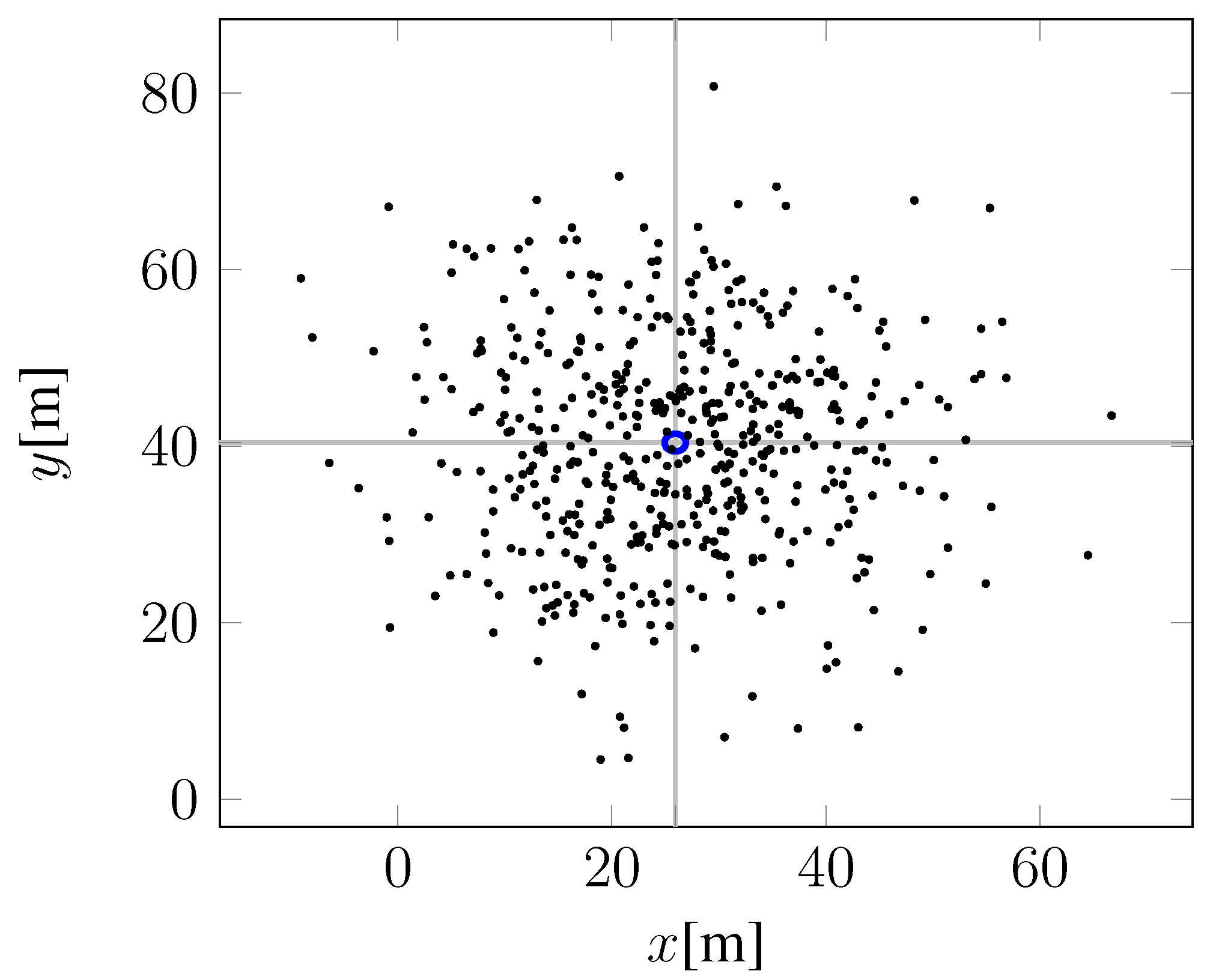
4.5. Planning Quality


4.6. Transfer of Planning

4.7. Discussion of the Results
5. Evaluation of Reasoning for Learning
5.1. Experimental Setup
- elbow joint at start/end configuration
- wrist joint at start/end configuration
- time in which the action is to be performed

5.2. QSL-Based Task Specification for Filtering
5.2.1. Proper Throw
5.2.2. Throwing to the Front
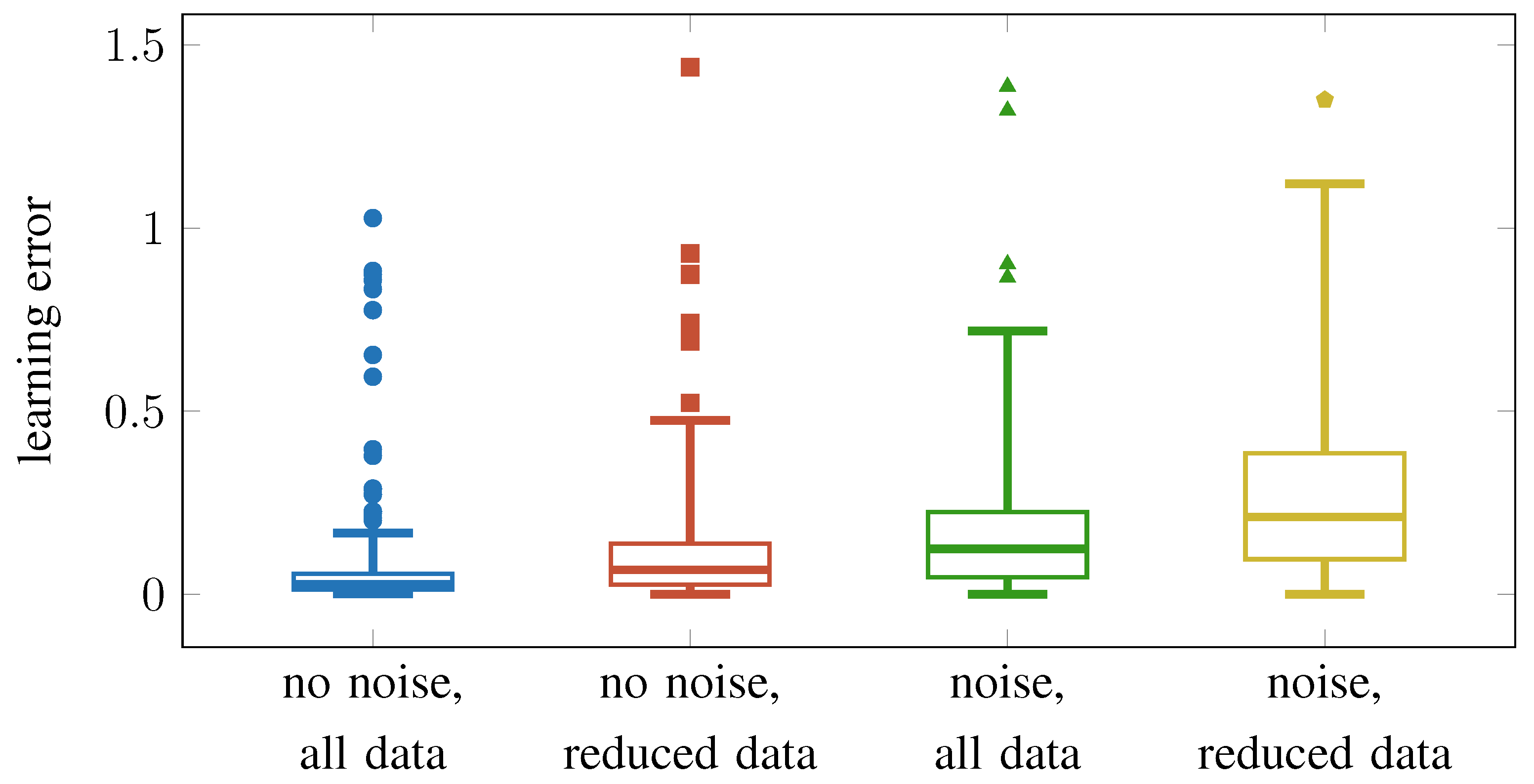
5.3. Learning Performance
| Used | Number of | Learning Errors | |
|---|---|---|---|
| Filter | Training Instances | MAE | RMSE |
| none | 158 | 0.2092 | 0.2565 |
| radius (Equation (8)) | 88 | 0.1021 | 0.1457 |
| frontal (Equation (9)) | 125 | 0.2217 | 0.2677 |
| radius + frontal | 80 | 0.0939 | 0.136 |
| Used | Number of | Learning Errors | |
|---|---|---|---|
| Filter | Training Instances | MAE | RMSE |
| none | 158 | 0.8058 | 1.431 |
| radius (Equation (8)) | 88 | 0.4164 | 1.1046 |
| frontal (Equation (9)) | 125 | 0.0156 | 0.0279 |
| radius + frontal | 80 | 0.0103 | 0.0178 |
6. Discussion
6.1. Discussion of Related Approaches
7. Conclusions
Acknowledgments
Author Contributions
Conflicts of Interest
References
- Williams, B.C.; de Kleer, J. Qualitative Reasoning About Physical Systems—A Return to Roots. Artif. Intell. 1991, 51, 1–9. [Google Scholar] [CrossRef]
- Bredeweg, B.; Struss, P. Current topics in qualitative reasoning. AI Mag. 2003, 24, 13–16. [Google Scholar]
- Davis, E. Representations of Commonsense Knowledge; Morgan Kaufmann Series in Representation and Reasoning; Morgan Kaufmann Publishers: San Mateo, CA, USA, 1990. [Google Scholar]
- Mösenlechner, L.; Beetz, M. Parameterizing Actions to have the Appropriate Effects. In Proceedings of the IEEE/RSJ International Conference on Intelligent Robots and Systems (IROS), San Francisco, CA, USA, 25–30 September 2011.
- Knauff, M.; Strube, G.; Jola, C.; Rauh, R.; Schlieder, C. The Psychological Validity of Qualitative Spatial Reasoning in One Dimension. Spat. Cogn. Comput. 2004, 4, 167–188. [Google Scholar] [CrossRef]
- Kirsch, A. Robot Learning Language—Integrating Programming and Learning for Cognitive Systems. Robot. Auton. Syst. J. 2009, 57, 943–954. [Google Scholar] [CrossRef]
- Hall, M.; Frank, E.; Holmes, G.; Pfahringer, B.; Reutemann, P.; Witten, I.H. The WEKA Data Mining Software: An Update. SIGKDD Explor. 2009, 11, 10–18. [Google Scholar] [CrossRef]
- Echeverria, G.; Lassabe, N.; Degroote, A.; Lemaignan, S. Modular openrobots simulation engine: MORSE. In Proceedings of the IEEE International Conference on Robotics and Automation (ICRA), Shanghai, China, 9–13 May 2011.
- Lemaignan, S.; Echeverria, G.; Karg, M.; Mainprice, M.; Kirsch, A.; Alami, R. Human-Robot Interaction in the MORSE Simulator. In Proceedings of the 2012 7th ACM/IEEE International Conference on Human-Robot Interaction Conference (Late Breaking Report), Boston, MA, USA, 5–8 March 2012.
- Cohn, A.G.; Renz, J. Qualitative Spatial Representation and Reasoning. Chapter 13: Foundations of Artificial Intelligence. In Handbook of Knowledge Representation; Van Harmelen, F., Lifschitz, V., Porter, B., Eds.; Elsevier: Amsterdam, The Netherlands, 2008; Volume 3, pp. 551–596. [Google Scholar]
- Kontchakov, R.; Kurucz, A.; Wolter, F.; Zakharyaschev, M. Spatial Logic + Temporal Logic = ? In Handbook of Spatial Logics; Aiello, M., Pratt-Hartmann, I.E., van Benthem, J.F., Eds.; Springer: Dordrecht, The Netherlands, 2007; pp. 497–564. [Google Scholar]
- Vilain, M.B.; Kautz, H.A. Constraint propagation algorithms for temporal reasoning. In Proceedings of the 5th National Conference of the 13 American Association for Artificial Intelligence (AAAI-86), Philadelphia, PA, USA, 11–15 August 1986; pp. 377–382.
- Allen, J.F. Maintaining knowledge about temporal intervals. Commun. ACM 1983, 26, 832–843. [Google Scholar] [CrossRef]
- Balbiani, P.; Condotta, J.; Fariñas del Cerro, L. Tractability Results in the Block Algebra. J. Logic Comput. 2002, 12, 885–909. [Google Scholar] [CrossRef]
- Renz, J.; Mitra, D. Qualitative Direction Calculi with Arbitrary Granularity. In Proceedings of the 8th Pacific Rim International Conference on Artificial Intelligence (PRICAI-04), Auckland, New Zealand, 9–13 August 2004; Volume 3157, pp. 65–74.
- Lee, J.H.; Renz, J.; Wolter, D. StarVars—Effective Reasoning about Relative Directions. In Proceedings of the Internatoinal Joint Conference on Artificial Intelligence (IJCAI), Beijing, China, 3–9 August 2013; Rossi, F., Ed.; AAAI Press: Palo Alto, California, 2013; pp. 976–982. [Google Scholar]
- Moratz, R.; Ragni, M. Qualitative spatial reasoning about relative point position. J. Vis. Lang. Comput. 2008, 19, 75–98. [Google Scholar] [CrossRef]
- Ligozat, G.; Renz, J. What Is a Qualitative Calculus? A General Framework. In Proceedings of the 8th Pacific Rim International Conference on Artificial Intelligence (PRICAI-04), Auckland, New Zealand, 9–13 August 2004; Zhang, C., Guesgen, H., Yeap, W., Eds.; Volume 3157, pp. 53–64.
- Dylla, F.; Mossakowski, T.; Schneider, T.; Wolter, D. Algebraic Properties of Qualitative Spatio-temporal Calculi. In Proceedings of the 11th International Conference on COSIT, Scarborough, UK, 2–6 September 2013; Volume 8116, pp. 516–536.
- Kreutzmann, A.; Wolter, D. Qualitative Spatial and Temporal Reasoning with AND/OR Linear Programming. In Proceedings of the 21st European Conference on Artificial Intelligence (ECAI), Prague, Czech, 17–22 August 2014.
- Pnueli, A. The temporal logic of programs. In Proceedings of the 18th Annual Symposium on Foundations of Computer Science (FOCS), Providence, RI, USA, 31 October–2 November 1977; pp. 46–57.
- Antoniotti, M.; Mishra, B. Discrete event models + temporal logic = supervisory controller: Automatic synthesis of locomotion controllers. In Proceedings of the IEEE Conference on Robotics and Automation (ICRA), Nagoya, Japan, 21–27 May 1995; Volume 2, pp. 1441–1446.
- Kress-Gazit, H.; Wongpiromsarn, T.; Topcu, U. Correct, Reactive Robot Control from Abstraction and Temporal Logic Specifications. Spec. Issue IEEE Robot. Autom. Mag. Form. Methods Robot. Autom. 2011, 18, 65–74. [Google Scholar] [CrossRef]
- Kloetzer, M.; Belta, C. LTL planning for groups of robots. In Proceedings of the IEEE International Conference on Networking, Sensing and Control (ICNSC), Ft. Lauderdale, FL, USA, 23–25 April 2006; pp. 578–583.
- Smith, S.L.; Tůmová, J.; Belta, C.; Rus, D. Optimal path planning under temporal logic constraints. In Proceeding of the IEEE/RSJ International Conference on Intelligent Robots and Systems (IROS), Taipei, Taiwan, 18–22 October 2010; pp. 3288–3293.
- Kloetzer, M.; Belta, C. Automatic deployment of distributed teams of robots from temporal logic motion specifications. IEEE Trans. Robot. 2010, 26, 48–61. [Google Scholar] [CrossRef]
- Kreutzmann, A.; Colonius, I.; Wolter, D.; Dylla, F.; Frommberger, L.; Freksa, C. Temporal logic for process specification and recognition. Intell. Serv. Robot. 2013, 6, 5–18. [Google Scholar] [CrossRef]
- Kröger, F.; Merz, S. Temporal Logic and State Systems; Texts in Theoretical Computer Science; Springer: Berlin Heidelberg, 2008. [Google Scholar]
- Bauland, M.; Mundhenk, M.; Schneider, T.; Schnoor, H.; Schnoor, I.; Vollmer, H. The tractability of model checking for LTL: The good, the bad, and the ugly fragments. Electron. Notes Theor. Comput. Sci. 2009, 231, 277–292. [Google Scholar] [CrossRef]
- Gebser, M.; Grote, T.; Schaub, T. Coala: A Compiler from Action Languages to ASP. In Lecture Notes in Computer Science In Proceedings of the 12th European Conference on Logics in Artificial Intelligence (JELIA), Helsinki, Finland, 13–15 September 2010; Volume 6341, pp. 360–364.
- Grosu, R.; Smolka, S.A. Monte Carlo Model Checking. In Tools and Algorithms for the Construction and Analysis of Systems; Springer: Berlin Heidelberg, 2005; Volume 3440, pp. 271–286. [Google Scholar]
- Witten, I.H.; Frank, E. Data Mining: Practical Machine Learning Tools and Techniques, 2nd ed.; Morgan Kaufmann: San Francisco, CA, USA, 2005. [Google Scholar]
- Quigley, M.; Conley, K.; Gerkey, B.; Faust, J.; Foote, T.; Leibs, J.; Wheeler, R.; Ng, A.Y. ROS: An open-source Robot Operating System. In Proceedings of the ICRA Workshop on Open Source Software, Kobe, Japan, 17 May 2009.
- Kirsch, A.; Schweitzer, M.; Beetz, M. Making Robot Learning Controllable: A Case Study in Robot Navigation. In Proceedings of the ICAPS Workshop on Plan Execution: A Reality Check, Monterey, CA, USA, 5–10 June 2005.
- Frommberger, L. Learning to Behave in Space: A Qualitative Spatial Representation for Robot Navigation with Reinforcement Learning. Int. J. Artif. Intell. Tools (IJAIT) 2008, 17, 465–482. [Google Scholar] [CrossRef]
- Kulick, J.; Toussaint, M.; Lang, T.; Lopes, M. Active Learning for Teaching a Robot Grounded Relational Symbols. In Proceedings of the International Joint Conference on Artificial Intelligence, IJCAI, Beijing, China, 3–9 August 2013.
- Beetz, M.; Mösenlechner, L.; Tenorth, M. CRAM—A Cognitive Robot Abstract Machine for Everyday Manipulation in Human Environments. In Proceedings of the International Conference on Intelligent Robots and Systems, Taipei, Taiwan, 18–22 October 2010; pp. 1012–1017.
- Tenorth, M.; Perzylo, A.C.; Lafrenz, R.; Beetz, M. Representation and Exchange of Knowledge about Actions, Objects, and Environments in the RoboEarth Framework. IEEE Trans. Autom. Sci. Eng. (T-ASE) 2013, 10, 643–651. [Google Scholar] [CrossRef]
- Tenorth, M.; Bartels, G.; Beetz, M. Knowledge-based Specification of Robot Motions. In Proceedings of the 21st European Conference on Artificial Intelligence (ECAI 2014), Prague, Czech, 18–22 August 2014.
- Levesque, H.J.; Reiter, R.; Lespérance, Y.; Lin, F.; Scherl, R.B. Golog: A logic programming language for dynamic domains. J. Logic Program. 1997, 31, 59–83. [Google Scholar] [CrossRef]
- Levesque, H.; Lakemeyer, G. Cognitive robotics. In Handbook of Knowledge Representation; Lifschitz, V., van Harmelen, F., Porter, F., Eds.; Elsevier: Amsterdam, The Netherlands, 2007. [Google Scholar]
- Mitchell, T. The Discipline of Machine Learning; Technical Report CMU-ML-06-108; Carnegie Mellon University: Pittsburgh, PA, USA, 2006. [Google Scholar]
- Kirsch, A. Integration of Programming and Learning in a Control Language for Autonomous Robots Performing Everyday Activities. Ph.D. Thesis, Technische Universität München, Munich, Germany, 2008. [Google Scholar]
- Thrun, S. Towards programming tools for robots that integrate probabilistic computation and learning. In Proceedings of the IEEE International Conference on Robotics and Automation (ICRA), San Francisco, CA, USA, 24–28 April 2000.
- Thrun, S. A Framework for Programming Embedded Systems: Initial Design and Results; Technical Report CMU-CS-98-142; Carnegie Mellon University, Computer Science Department: Pittsburgh, PA, USA, 1998. [Google Scholar]
- Andre, D.; Russell, S. Programmable Reinforcement Learning Agents. In Proceedings of the 13th Conference on Neural Information Processing Systems, Vancouver, BC, Canada, 3–8 December 2001; MIT Press: Cambridge, MA, USA, 2001; pp. 1019–1025. [Google Scholar]
- Andre, D. Programmable Reinforcement Learning Agents. Ph.D. Thesis, University of California, Berkeley, CA, USA, 2003. [Google Scholar]
© 2015 by the authors; licensee MDPI, Basel, Switzerland. This article is an open access article distributed under the terms and conditions of the Creative Commons Attribution license (http://creativecommons.org/licenses/by/4.0/).
Share and Cite
Wolter, D.; Kirsch, A. Leveraging Qualitative Reasoning to Learning Manipulation Tasks. Robotics 2015, 4, 253-283. https://doi.org/10.3390/robotics4030253
Wolter D, Kirsch A. Leveraging Qualitative Reasoning to Learning Manipulation Tasks. Robotics. 2015; 4(3):253-283. https://doi.org/10.3390/robotics4030253
Chicago/Turabian StyleWolter, Diedrich, and Alexandra Kirsch. 2015. "Leveraging Qualitative Reasoning to Learning Manipulation Tasks" Robotics 4, no. 3: 253-283. https://doi.org/10.3390/robotics4030253
APA StyleWolter, D., & Kirsch, A. (2015). Leveraging Qualitative Reasoning to Learning Manipulation Tasks. Robotics, 4(3), 253-283. https://doi.org/10.3390/robotics4030253