
Navigation of an Autonomous Tractor for a Row-Type Tree Plantation Using a Laser Range Finder—Development of a Point-to-Go Algorithm


Abstract
: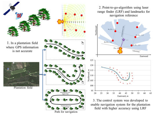
1. Introduction


2. Materials and Methods
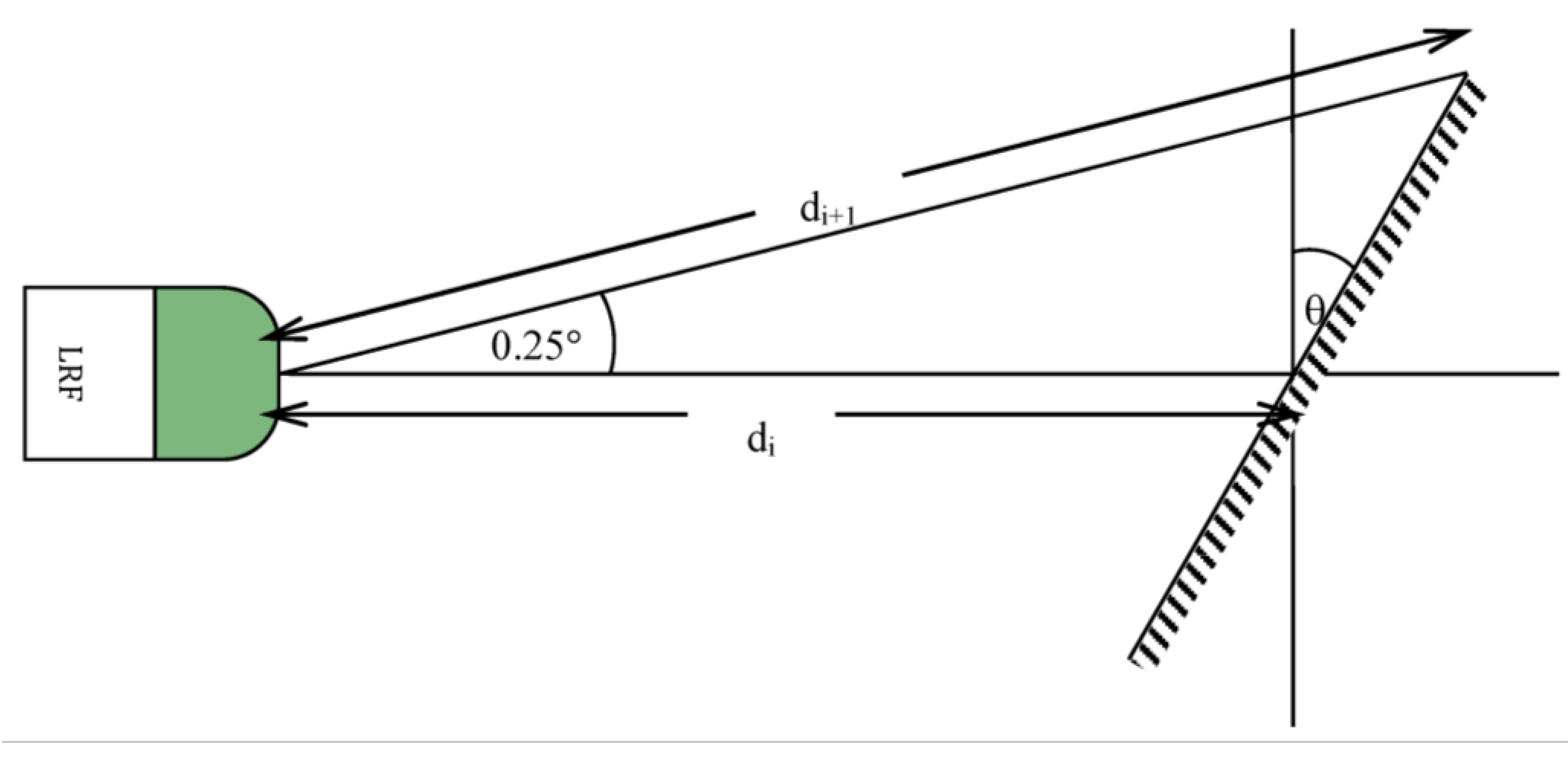
2.1. Instrument Setup

2.2. Navigation Control Algorithm

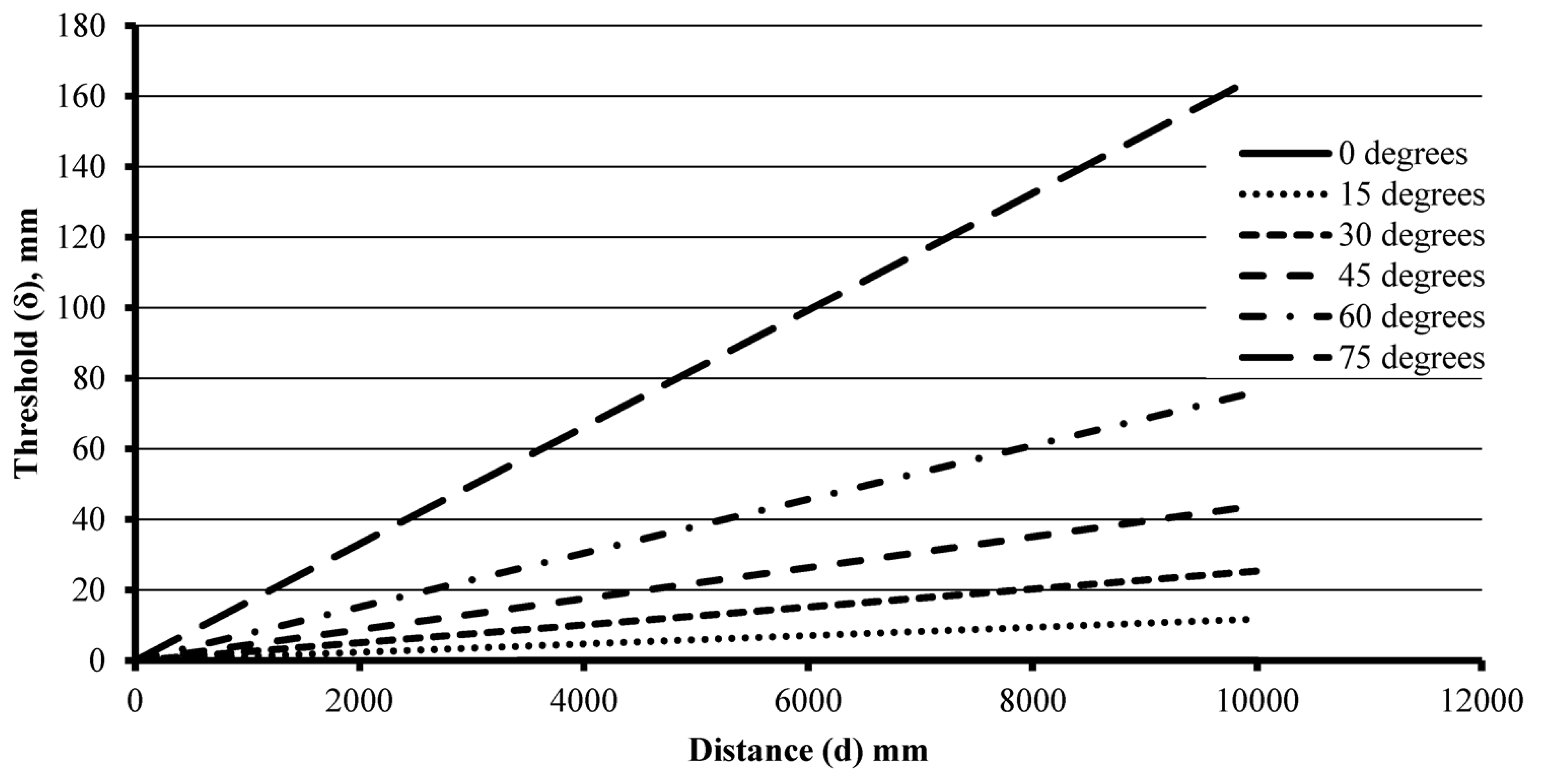
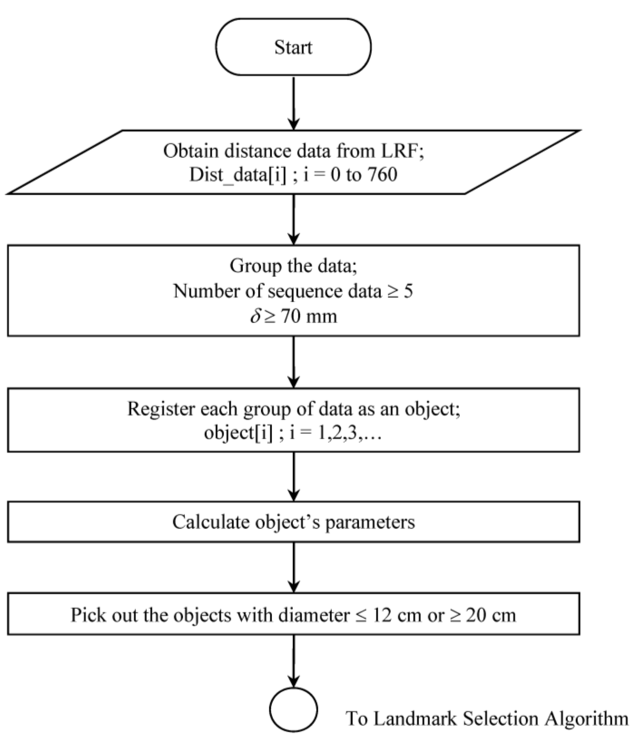
2.2.1. Object Extraction


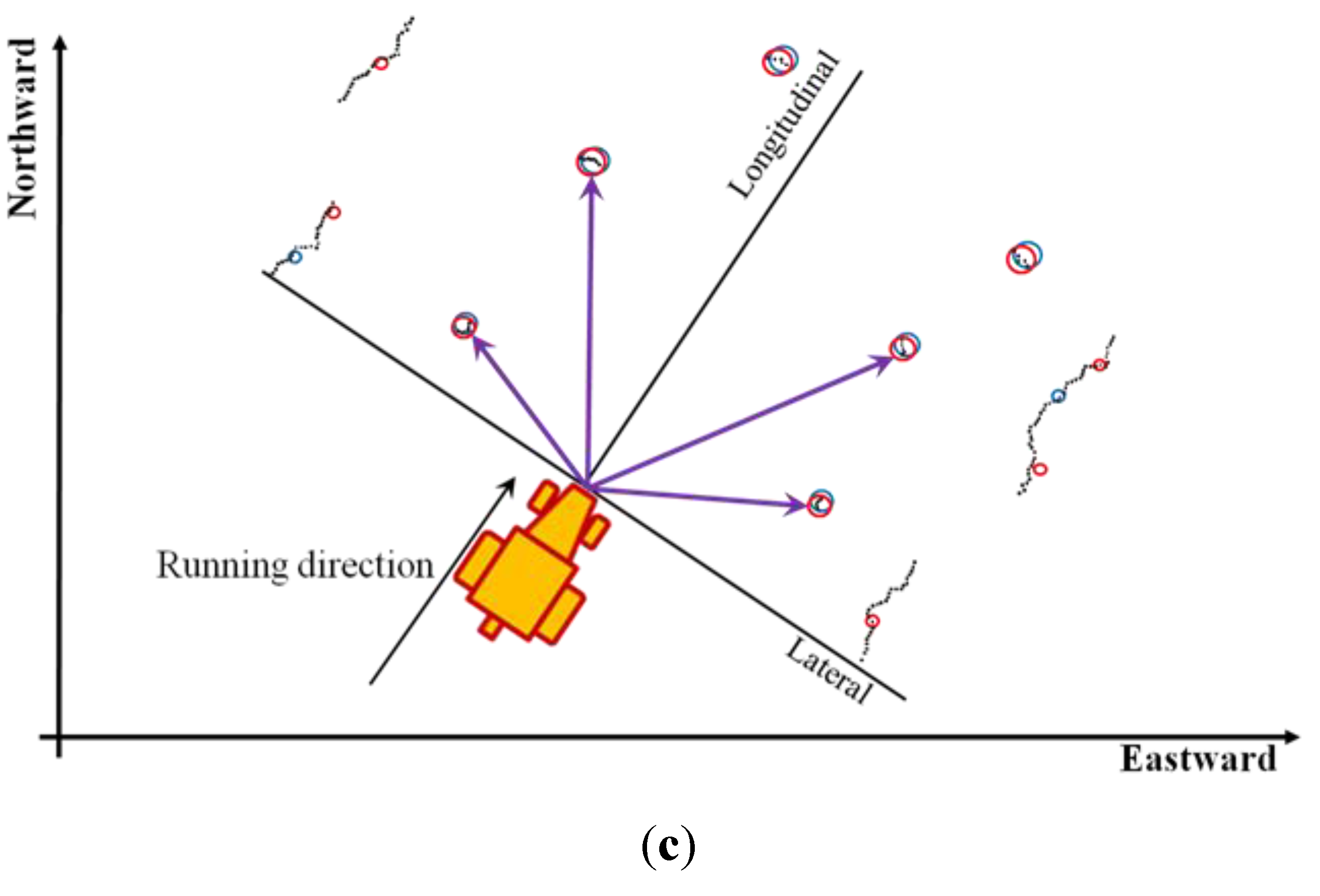
2.2.2. Landmark Selection from Extracted Objects

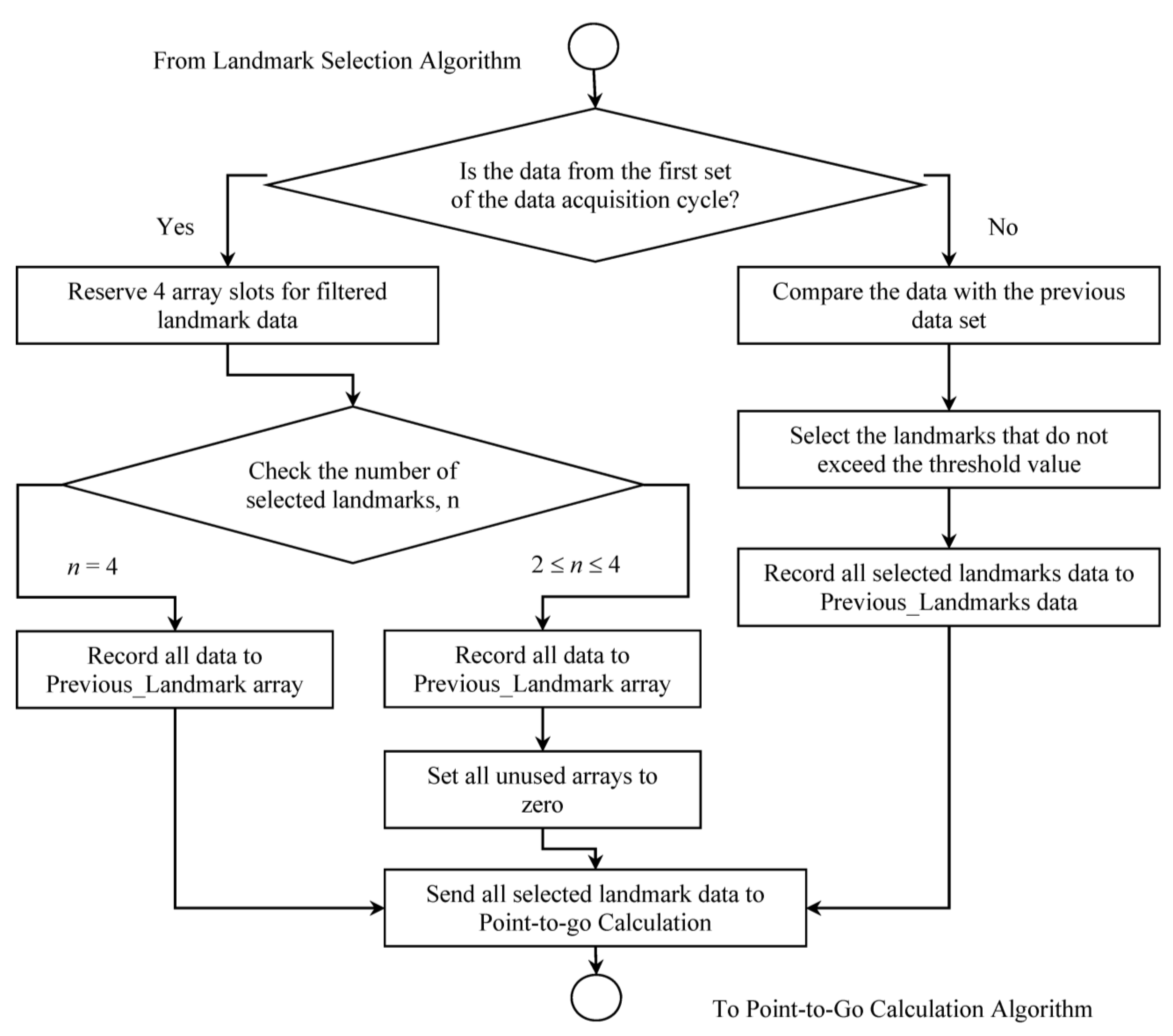
2.2.3. Landmark Selection Filtering


2.2.4. Point-to-Go Calculation


2.2.5. Steering Control

2.3. Navigation Using Landmarks
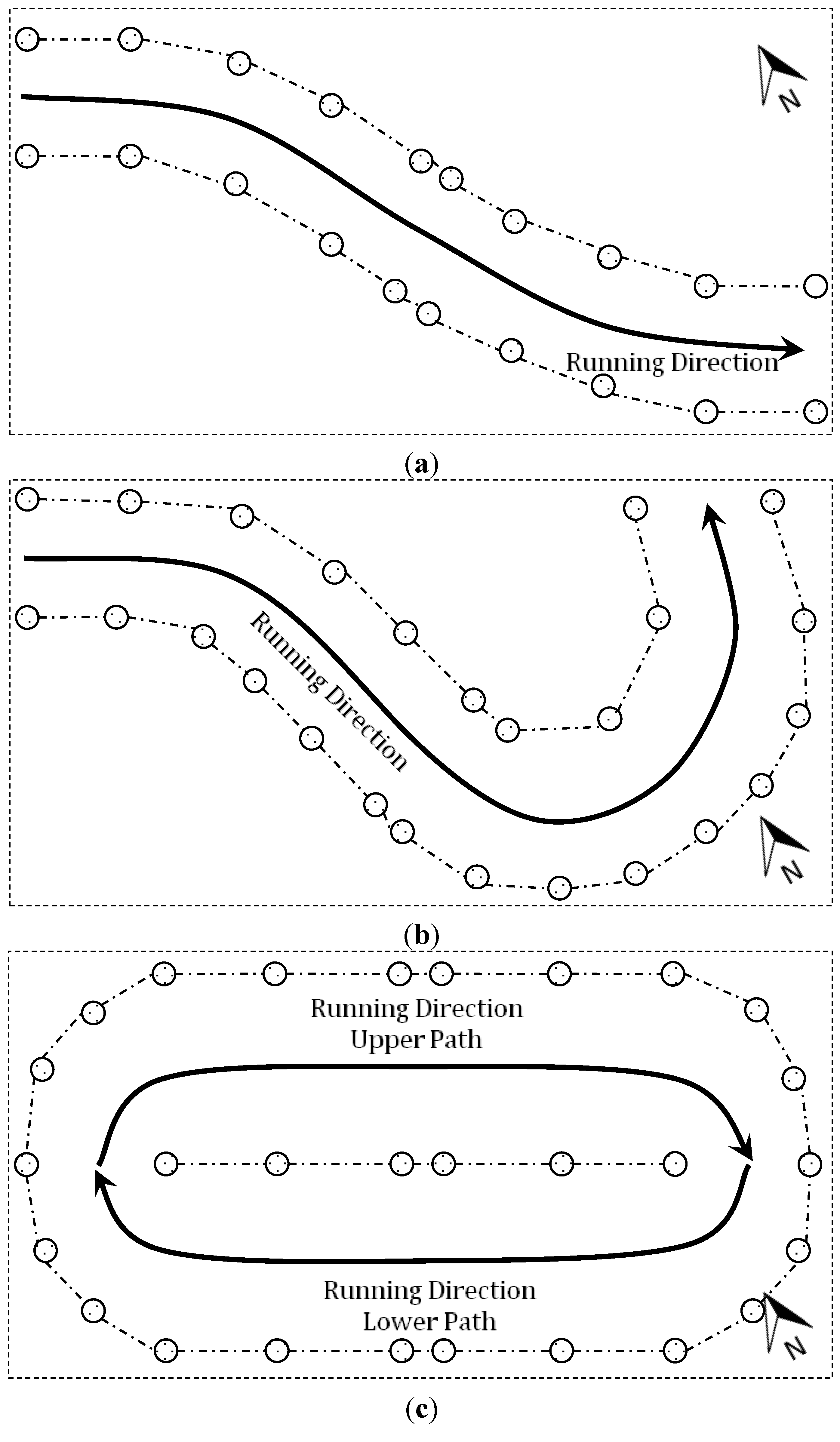
2.3.1. Experimental Paths


2.3.2. Accuracy of the Control System
3. Results
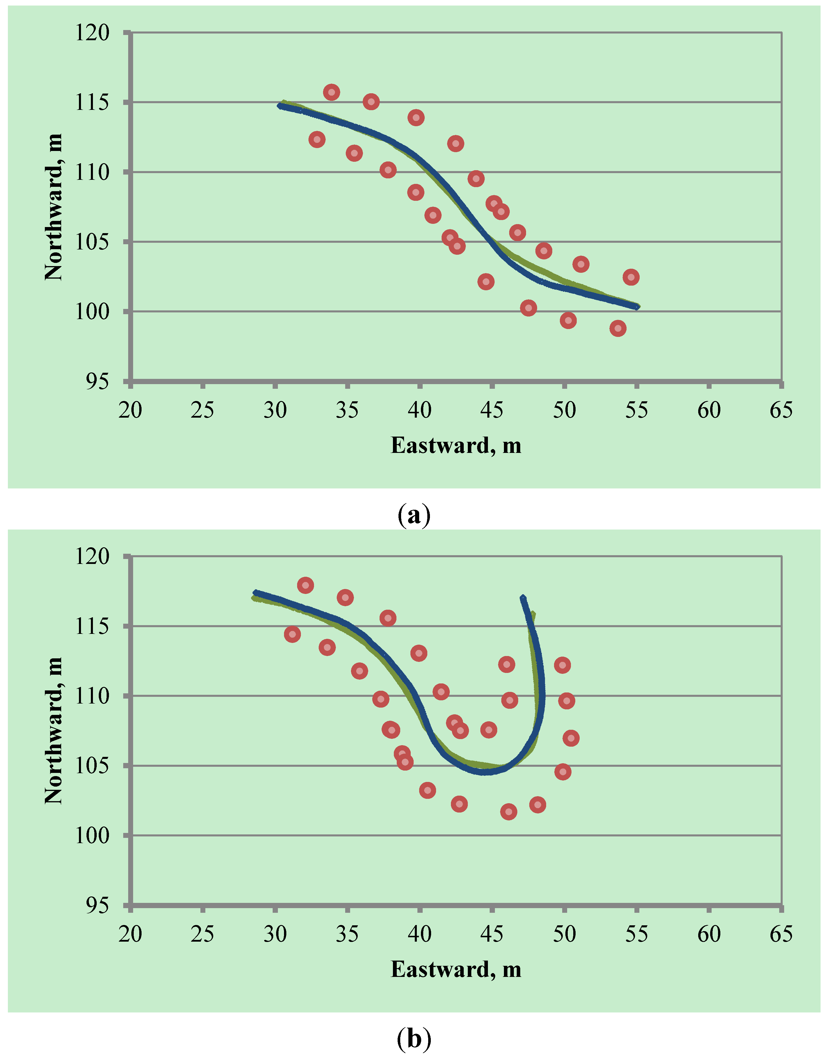
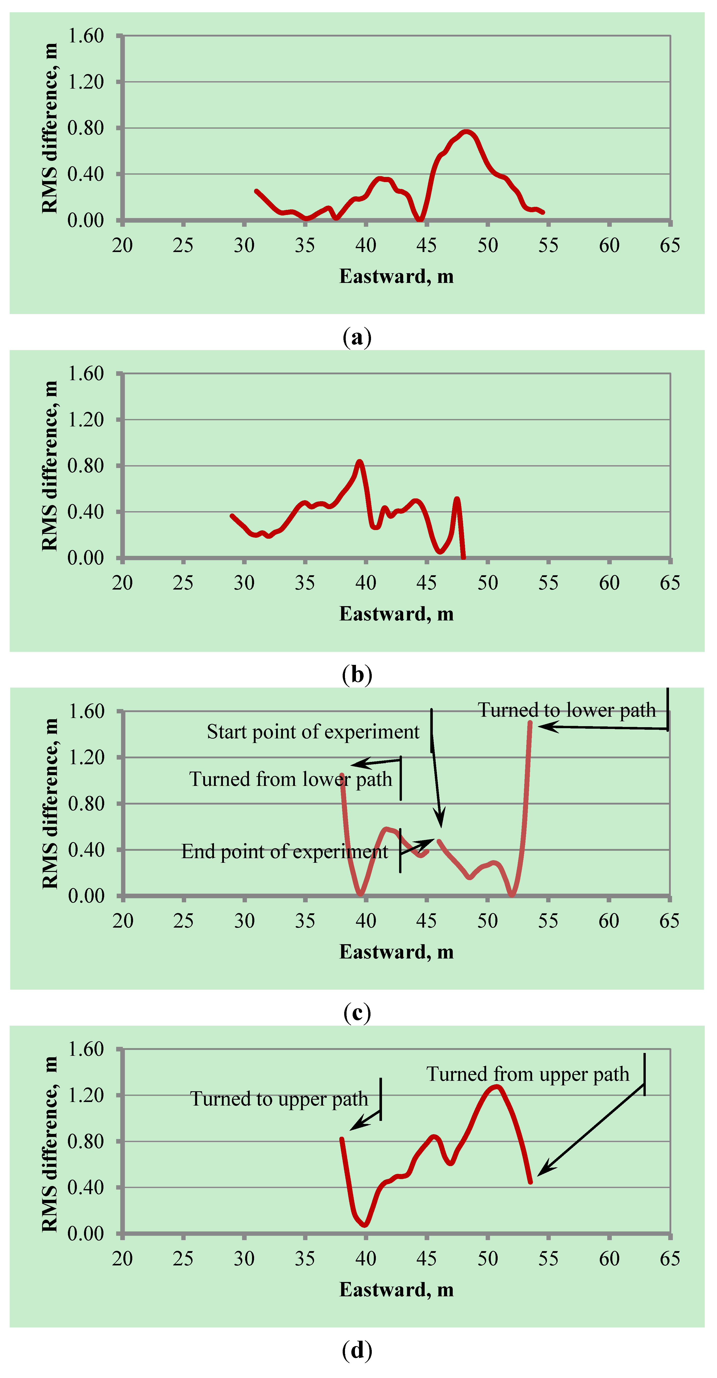
3.1. Comparison of Path Execution for Manual and Autonomous Runs


| Test Course | Average RMS Position Difference, m |
|---|---|
| Test course 1 (wide curve) | 0.264 |
| Test course 2 (tight curve) | 0.370 |
| Test course 3 (U-turn run) | 0.542 |
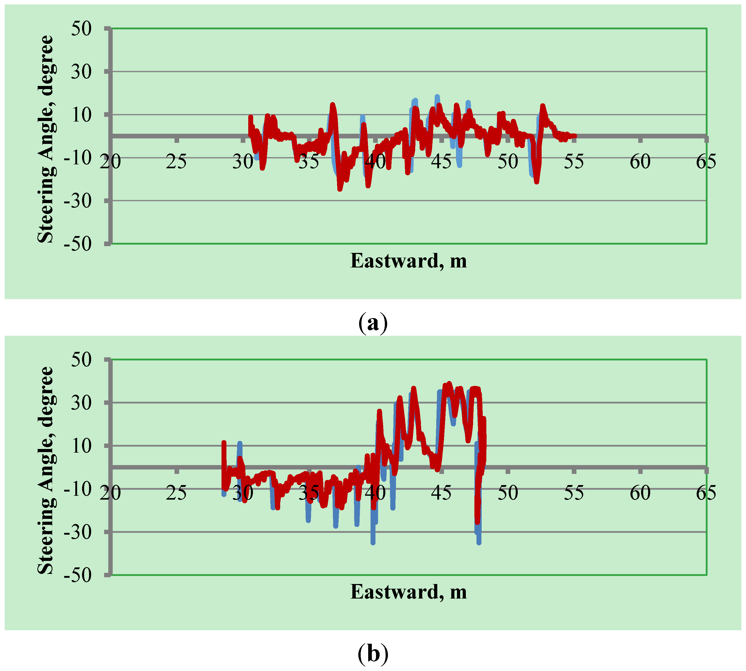
3.2. Performance Evaluation of Steering Angle


| Test Course | Average RMS Position Difference, Degree |
|---|---|
| Test course 1 (wide curve) | 3.139 |
| Test course 2 (tight curve) | 4.394 |
| Test course 3 (U-turn run) | 5.217 |
4. Discussion
5. Conclusions
Author Contributions
Conflicts of Interest
References
- O’Conner, M.; Bell, T.; Elkaim, G.; Parkinson, B. Automatic steering of farm vehicles using GPS. In Proceedings of the Third International Conference on Precision Agriculture, Minneapolis, MN, USA, 23–26 June 1996; pp. 767–778.
- O’Connor, M.; Elkaim, G.H.; Parkinson, B.W. Carrier-phase DGPS for closed-loop control of farm and construction vehicles. J. Inst. Navig. 1996, 43, 167–178. [Google Scholar] [CrossRef]
- Stombaugh, T.S.; Bensen, E.R.; Hummel, J.W. Guidance of agricultural vehicles at high field speeds. Trans. ASABE 1999, 42, 537–544. [Google Scholar] [CrossRef]
- Van Zuydam, R.P. A driver’s steering aid for an agricultural implement, based on an electronic map and real time kinematic DGPS. Comput. Electron. Agric. 1999, 24, 153–163. [Google Scholar] [CrossRef]
- Bell, T. Automatic tractor guidance using carrier-phase differential GPS. Comput. Electron. Agric. 2000, 25, 53–66. [Google Scholar] [CrossRef]
- Nagasaka, Y.; Umeda, N.; Kanetai, Y.; Taniwaki, K.; Sasaki, Y. Autonomous guidance for rice transplanting using global positioning and gyroscopes. Comput. Electron. Agric. 2004, 43, 223–234. [Google Scholar] [CrossRef]
- Casciati, F.; Domanesshi, M.; Faravelli, L. Design and implementation of a pointer system controller. Nonlinear Dyn. 2004, 36, 203–215. [Google Scholar] [CrossRef]
- Casciati, F.; Fuggini, C. Monitoring a steel building using GPS sensors. Smart Struct. Syst. 2011, 7, 349–363. [Google Scholar] [CrossRef]
- Wu, L.; Casciati, F. Local positioning systems versus structural monitoring: A review. Struct. Control Health Monit. 2014, 21, 1209–1221. [Google Scholar] [CrossRef]
- Barawid, O.C., Jr.; Mizushima, A.; Ishii, K.; Noguchi, N. Development of an autonomous navigation system using a two-dimensional laser scanner in an orchard application. Biosyst. Eng. 2007, 96, 139–149. [Google Scholar] [CrossRef]
- Ahamed, T.; Tian, L.; Takigawa, T.; Zhang, Y. Development of auto-hitching navigation system for farm implements using laser range finder. Trans. ASABE 2009, 52, 1793–1803. [Google Scholar] [CrossRef]
- Ahamed, T.; Takigawa, T.; Koike, M.; Honma, T.; Hasegawa, H.; Zhang, Q. Navigation using a laser range finder for autonomous tractor (part 1)—Positioning of implement. J. JSAM 2006, 68, 68–77. [Google Scholar]
- Ahamed, T.; Takigawa, T.; Koike, M.; Honma, T.; Hasegawa, H.; Zhang, Q. Navigation using a laser range finder for autonomous tractor (part 2)—Navigation for approach composed of multiple paths. J. JSAM 2006, 68, 78–86. [Google Scholar]
- Takigawa, T.; Sutiarso, L.; Koike, M.; Kurosaki, H.; Hasegawa, H. Trajectory control and its application to approach a target: Part I. Development of trajectory control algorithms for an autonomous vehicle. Trans. ASAE 2002, 45, 1191–1197. [Google Scholar] [CrossRef]
- Sutiarso, L.; Kurosaki, H.; Takigawa, T.; Koike, M.; Yukumoto, O.; Hasegawa, H. Trajectory control and its application to approach a target: Part II. Target approach experiments. Trans. ASAE 2002, 45, 1199–1205. [Google Scholar] [CrossRef]
- Hamner, B.; Bergerman, M.; Singh, S. Autonomous orchard vehicles for specialty crops production. In ASABE Annual International Meeting; ASABE: Louisville, KY, USA, 2011. [Google Scholar]
- Zhang, J.; Chambers, A.; Maeta, S.; Bergerman, M.; Singh, S. 3D perception for accurate row following: Methodology and results. In Proceedings of the IEEE/RSJ International Conference on Intelligent Robots and Systems (IROS), Tokyo, Japan, 3–7 November 2013.
- Subramanian, V.; Burks, T.F.; Arroyo, A.A. Development of machine vision and laser radar based autonomous vehicle guidance systems for citrus grove navigation. Comput. Electron. Agric. 2006, 53, 130–143. [Google Scholar] [CrossRef]
- Choi, J.; Yin, X.; Yang, L.; Noguchi, N. Development of a laser scanner-based navigation system for a combine harvester. Eng. Agric. Environ. Food 2014, 7, 7–13. [Google Scholar] [CrossRef]
- Kurashiki, K.; Fukao, T.; Nagata, J.; Ichiyama, K.; Kamiya, T.; Murakami, N. Orchard travelling ugv using a laser range finder based localization and inverse optimal control. J. Robot. Soc. Jpn. 2014, 30, 428–435. [Google Scholar] [CrossRef]
- Thanpattranon, P.; Takigawa, T. An application of laser range finder for tractor-trailer navigation in mountainous area, experiment on artifact pathway. In Proceedings of the 69th Japanese Society of Agricultural Machinery Annual Meeting, Ehime, Japan, 14–15 September 2010; pp. 70–71.
- Thanpattranon, P.; Takigawa, T. Tractor steering control using laser range finder. In Proceedings of the 70th Japanese Society of Agricultural Machinery Annual Meeting, Aomori, Japan, 27–28 September 2011; pp. 244–245.
© 2015 by the authors; licensee MDPI, Basel, Switzerland. This article is an open access article distributed under the terms and conditions of the Creative Commons Attribution license (http://creativecommons.org/licenses/by/4.0/).
Share and Cite
Thanpattranon, P.; Ahamed, T.; Takigawa, T. Navigation of an Autonomous Tractor for a Row-Type Tree Plantation Using a Laser Range Finder—Development of a Point-to-Go Algorithm. Robotics 2015, 4, 341-364. https://doi.org/10.3390/robotics4030341
Thanpattranon P, Ahamed T, Takigawa T. Navigation of an Autonomous Tractor for a Row-Type Tree Plantation Using a Laser Range Finder—Development of a Point-to-Go Algorithm. Robotics. 2015; 4(3):341-364. https://doi.org/10.3390/robotics4030341
Chicago/Turabian StyleThanpattranon, Pawin, Tofael Ahamed, and Tomohiro Takigawa. 2015. "Navigation of an Autonomous Tractor for a Row-Type Tree Plantation Using a Laser Range Finder—Development of a Point-to-Go Algorithm" Robotics 4, no. 3: 341-364. https://doi.org/10.3390/robotics4030341
APA StyleThanpattranon, P., Ahamed, T., & Takigawa, T. (2015). Navigation of an Autonomous Tractor for a Row-Type Tree Plantation Using a Laser Range Finder—Development of a Point-to-Go Algorithm. Robotics, 4(3), 341-364. https://doi.org/10.3390/robotics4030341