Static Stability Analysis of a Planar Object Grasped by Multifingers with Three Joints

Abstract

This paper discusses static stability of a planar object grasped by multifingers with three joints. Each individual joint (prismatic joint or revolute joint) is modeled as a linear spring stiffness. The object mass and the link masses are also included. We consider not only pure rolling contact but also frictionless sliding contact. The grasp stability is investigated using the potential energy method. This paper makes the following contributions: (i) Grasp wrench vectors and grasp stiffness matrices are analytically derived not only for the rolling contact but also for the sliding contact; (ii) It is shown in detail that the vectors and the matrices are given by functions of grasp parameters such as the contact conditions (rolling contact and sliding contact), the contact position, the contact force, the local curvature, the link shape, the object mass, the link masses, and so on; (iii) By using positive definiteness of the difference matrix of the grasp stiffness matrices, it is analytically proved that the rolling contact grasp is more stable than the sliding contact grasp. The displacement direction affected by the contact condition deviation is derived; (iv) By using positive definiteness of the differential matrix with respect to the local curvatures, it is analytically proved that the grasp stability increases when the local curvatures decrease. The displacement direction affected by the local curvature deviation is also derived; (v) Effects of the object mass and the joint positions are discussed using numerical examples. The numerical results are reinforced by analytical explanations. The effect of the link masses is also investigated.

1. Introduction

Human beings can grasp and manipulate various shaped objects dexterously. For this reason, handling skills inherent in human nature are required for accomplishing assembly tasks including complicated shaped objects and complicated contact conditions. It is required that production lines are automatized using robot systems in order to improve working conditions and maintain constant and high quality productions. Multi-fingered robot hands are useful for the handling tasks of various shaped objects. Grasp stability is an important factor for dexterous grasp and manipulation using the hands. While external forces are applied to the grasp and the object pose is displaced, the grasp has to be unbreakable and the robots have to accomplish the handling and assembly tasks. The grasp stability has been investigated in many works (Table 1).

Table 1. Differences among the previous works.

	Dimensions	Local Curvature of the Finger Surface	Curvature Deviation (Positive Definiteness)	Contact Condition	Contact Condition Diff. (Positive Definiteness)	Joint Stiffness	Nr. of Links	Link Mass	Mass Deviation
Hanafusa [1]	2D	-	-	PC	-	-	-	-	-
Nguyen [2]	3D	-	-	PC, PCWF,	-	-	-	-	-
Li [3]	3D	-	-	PCWF	-	-	-	-	-
Cutkosky [4]	3D	-	-	PCWF	-	O	O	-	-
Carbone [5]	3D	-	-	PCWF	-	O	O	-	-
Kim [6]	3D	-	-	PCWF	-	-	O	-	-
Babiccini [7]	3D	-	-	PCWF	-	-	-	-	-
Malvezzi [8]	2D	-	-	PCWF	-	-	-	-	-
Shapiro [9]	3D	-	-	PC	-	-	-	-	-
Montana [10]	3D	included	-	RC	-	-	-	-	-
Xiong [11]	3D	included	-	RC	-	-	-	-	-
Choi [12]	3D	included	-	RC	-	-	-	-	-
Michalec [13]	3D	included	-	RC	-	-	O	O	-
Funahashi [14]	2D	included	-	RC, SC(1D)	-	-	-	-	-
Howard [15]	3D	included	-	RC, SC(1D)	-	O	O	-	-
Howard [16]	3D	included	-	RC, SC(1D)	-	-	-	-	-
Lin [17]	2D	included	-	SC(1D)	-	-	-	-	-
Yamada [18]	2D	included	-	RC, SC	-	-	-	-	-
Yamada [19,20,21]	3D	included	-	RC, SC	-	-	-	-	-
Yamada [22]	2D	included	treated	RC, SC	treated	O	2	-	-
This paper	2D	included	treated	RC, SC	treated	O	3	O	O

O: treated, -: Untreated, PC: Point contact without friction, PCWF: Point contact with friction, RC: Rolling contact, SC: Sliding contact, SC(1D): Sliding contact with a single spring model.

Table 1. Differences among the previous works.

	Dimensions	Local Curvature of the Finger Surface	Curvature Deviation (Positive Definiteness)	Contact Condition	Contact Condition Diff. (Positive Definiteness)	Joint Stiffness	Nr. of Links	Link Mass	Mass Deviation
Hanafusa [1]	2D	-	-	PC	-	-	-	-	-
Nguyen [2]	3D	-	-	PC, PCWF,	-	-	-	-	-
Li [3]	3D	-	-	PCWF	-	-	-	-	-
Cutkosky [4]	3D	-	-	PCWF	-	O	O	-	-
Carbone [5]	3D	-	-	PCWF	-	O	O	-	-
Kim [6]	3D	-	-	PCWF	-	-	O	-	-
Babiccini [7]	3D	-	-	PCWF	-	-	-	-	-
Malvezzi [8]	2D	-	-	PCWF	-	-	-	-	-
Shapiro [9]	3D	-	-	PC	-	-	-	-	-
Montana [10]	3D	included	-	RC	-	-	-	-	-
Xiong [11]	3D	included	-	RC	-	-	-	-	-
Choi [12]	3D	included	-	RC	-	-	-	-	-
Michalec [13]	3D	included	-	RC	-	-	O	O	-
Funahashi [14]	2D	included	-	RC, SC(1D)	-	-	-	-	-
Howard [15]	3D	included	-	RC, SC(1D)	-	O	O	-	-
Howard [16]	3D	included	-	RC, SC(1D)	-	-	-	-	-
Lin [17]	2D	included	-	SC(1D)	-	-	-	-	-
Yamada [18]	2D	included	-	RC, SC	-	-	-	-	-
Yamada [19,20,21]	3D	included	-	RC, SC	-	-	-	-	-
Yamada [22]	2D	included	treated	RC, SC	treated	O	2	-	-
This paper	2D	included	treated	RC, SC	treated	O	3	O	O

O: treated, -: Untreated, PC: Point contact without friction, PCWF: Point contact with friction, RC: Rolling contact, SC: Sliding contact, SC(1D): Sliding contact with a single spring model.

Hanafusa and Asada [1] discussed a planar object grasped by mechanical elastic fingers. It was shown that stable grasps are given at the minimum potential energy stored in the grasp. Nguyen [2] pointed out that the elastic fingers can be modeled as virtual linear springs. It was shown that stable grasps are given by using the gradient and the Hessian of the stored energy. That is, the equilibrium grasp is stable if the Hessian is positive definite. Such a Hessian is called a grasp stiffness matrix. In his analysis, the object shape is limited to a polyhedral object and the finger shape is a pointed finger. Li and Kao [3] discussed properties of the grasp stiffness matrix. Cutkosky and Kao [4] included joint compliance (joint stiffness) and formulated the grasp stiffness matrix. Carbone [5] discussed Cartesian stiffness matrices for various types of robot systems. Kim et al. [6] discussed task based compliance for peg-in-hole tasks and investigated a suitable grasp stiffness matrix. Gabiccini et al. [7] and Malvezzi and Prattichizzo [8] investigated the grasp stiffness in underactuated hands. Shapiro et al. [9] investigated force closure grasps and allowable external wrenches. In their analysis, local curvature parameters of the object surface or the finger surface were not included. This means that the local shape is assumed to be pointed.

Montana [10] pointed out that the local curvatures and the contact distance between contact points affect the grasp stability. The grasp was formulated as a dynamical system considering the surface curvatures. Xiong et al. [11] included contact stiffness and investigated dynamic grasp stability. Choi et al. [12] investigated the spatial grasp stiffness matrix considering the rolling contact and the local curvature. The elastic finger surface is replaced as spatial spring stiffness. Michalec and Micaelli [13] formulated the stiffness matrix considering joint stiffness, local curvature and rolling contact. They treated the rolling contact only.

Funahashi et al. [14] replaced every finger as the linear spring model and investigated the grasp stability from the stored energy. The finger and the object surfaces at contact points were approximate circles. Not only pure rolling contact but also frictionless sliding contact were investigated. Howard and Kumar [15,16] focused on the elastic property of the object and the finger. In the case of frictionless contact, the contact stiffness was modeled as a single spring along the initial contact normal direction. In the case of friction contact, the stiffness was replaced as a multiple-springs model. The spring stiffness and the local curvatures are included in the grasp stiffness matrix. Lin et al. [17] investigated the grasp stiffness matrix for immobility of the object. The finger is immobile and the contact stiffness is modeled as a single spring. This means that the contact is limited to frictionless contact and the finger is considered as a fixture part. In their formulations [6,7,8,9], the spring model was switched depending on the contact friction condition.

Yamada et al. [18] pointed out that the difference between the rolling contact and the sliding contact is represented not by the difference of the spring models but by the difference of contact point displacements on the object and the finger. The multiple-springs model was used not only for the rolling contact but also for the sliding contact. The relationship between the displacements of the object and the spring was formulated and the grasp stiffness matrix was derived. Yamada et al. [19,20,21] discussed spatial grasp stability with not only rolling contact but also sliding contact. In this analysis, the contact surface geometry (metric tensor, curvature, and torsion) was included. The wrench vector and the grasp stiffness matrix were analytically derived. Whereas References [18,19,20,21] did not consider the finger links, References [13,15] included the finger links but did not treat both the rolling and the sliding contacts with the same spring stiffness.

Yamada et al. [22] included the finger links and discussed the case that the fingers are constructed by revolute joints. The grasp stiffness matrix was formulated not only for the rolling contact but also for the sliding contact. In this analysis, the finger links are included but the number of links was restricted to two joints and the link masses were not considered. The effects of the object mass and the link masses on the stability were not investigated. In order for the rolling contact constraint to occur between the finger and the object, every finger requires at least two joints. Hence, Reference [22] employed two-joint fingers based on Reference [18].

In general, it is conceivable that an object is grasped by fingers or arms with three or more joints. In this paper, we discuss the case of three-joint fingers. Moreover, the object mass and the link masses are included. We investigate not only rolling contact but also sliding contact between the object and the fingers. The grasp stability is discussed by using the potential energy method. The wrench vectors and the grasp stiffness matrices are analytically derived. Grasp stability is evaluated by the eigenvalues and eigenvectors of the matrices. The vectors and the matrices are given by functions of grasp parameters such as the contact conditions (pure rolling and frictionless sliding), the local curvatures at contact points, contact forces, the masses, and so on. The effects of the contact conditions and the local curvatures on the stability are investigated by using positive definiteness of the grasp stiffness matrices. Effects of the object mass, the link masses, and the joint positions are investigated through numerical examples.

The analysis for frictionless sliding contact is applicable for the case that the friction coefficient of an object to be grasped is unknown beforehand, the object is covered with machine oil, or the surface property is slippery, similar to a cube of ice.

2. Problem Definitions

We suppose an object grasped by multifingers with three joints as shown in Figure 1. We analyze static stability of the grasp.

Figure 1. An object grasped by multifingers with three revolute joints.

Figure 1. An object grasped by multifingers with three revolute joints.

2.1. Assumptions

For simplicity of discussions, we analyze the stability based on the following assumptions:

(A1) The object and the fingers are rigid bodies;

(A2) A single point contact exists between two bodies;

(A3) Initial grasp pose (position and orientation) is given;

(A4) The local curvature at each contact point is given;

(A5) An infinitesimal pose displacement of the object occurs due to an external disturbance;

(A6) Each finger is constructed with three joints. The relationship between the joint torque and the joint position displacement is replaced with a linear stiffness.

Motion of the bodies is simplified from (A1) and (A2). If the material of the bodies is metal, its property is considered as rigid bodies described in (A1). If the object or the fingers are soft bodies, deformation of bodies has to be considered. In the case of soft bodies, the representation of the bodies’ motion is much more complicated. If two or more contact points exist between two bodies, the contact form is represented by a line contact or a face contact and degrees of freedom of finger motion decrease. The grasp stability is analyzed when the grasp parameters are given from (A3) and (A4). In our future work, we will discuss grasp position planning algorithms based on our stability analysis. From (A5), dynamics is not considered. Stability of the initial grasp is discussed by using the gradient and the Hessian of the stored potential energy. Our results are applicable for grasping an object in grasp planning or stabilizing or immobilizing an object in fixture position planning. The two-joints case was discussed in Reference [22]. If the number of joints is more than three, the joint Jacobian described in Section 3.3 is not a square matrix. Hence, the matrix is not invertible. In Assumption (A6), each joint is designed with passive stiffness joint or controlled by a compliance control. In three dimensional grasps, contact surface geometry (metric tensor, curvature, torsion) has to be included, joint position displacements and contact position displacements will be much more complicated. These cases will be addressed in our future work.

2.2. Nomenclature

We use the following coordinate frames (Figure 1 and Figure 2), ${\Sigma }_b$ is a base coordinate frame, ${\Sigma }_o$ is an object coordinate frame fixed in the object, ${\Sigma }_{Cok}$ and ${\Sigma }_{Cfk}$ are current contact coordinate frames moving on the object and the k-th finger surface, respectively. The frames ${\Sigma }_{\kappa ok}$ and ${\Sigma }_{\kappa fk}$ are curvature center coordinate frames of the contact point on the object and finger, respectively. The frames ${\Sigma }_{bo}$, ${\Sigma }_{Lfk}$, and ${\Sigma }_{Lok}$ are the initial coordinate frames of ${\Sigma }_o$, ${\Sigma }_{Cfk}$, and ${\Sigma }_{Cok}$, respectively.

Figure 2. Contact coordinate frames.

Figure 2. Contact coordinate frames.

The matrix ${}^{a}A_b\in {\text{R}}^{3\times 3}$ is a homogeneous transformation matrix of ${\Sigma }_b$ with respect to ${\Sigma }_a$. The vector ${}^a\mathit{p}_b\in {\text{R}}^2$ is the position component and the matrix ${}^{a}R_b\in {\text{R}}^{2\times 2}$ is the orientation component. Other vectors and matrices are also used.

$${}^{a}A_b:=\left[\begin{array}{cc}{}^{a}R_b& {}^a\mathit{p}_b\\ 0_{1\times 2}& 1\end{array}\right],{}^{a}B_b:=\left[\begin{array}{cc}{}^{a}R_b& -\Omega {}^a\mathit{p}_b\\ 0_{1\times 2}& 1\end{array}\right],{}^{a}W_b:=\left[\begin{array}{c}{}^{a}R_b\\ {}^a\mathit{p}_b\otimes {}^{a}R_b\end{array}\right]={[I_{23}{}^{b}B_a]}^T,A_t(\mathit{x}):=\left[\begin{array}{cc}{I}_2& \mathit{x}\\ 0_{1\times 2}& 1\end{array}\right],A_r(\zeta ):=\left[\begin{array}{cc}\mathrm{Rot}(\zeta )& 0_{2\times 1}\\ 0_{1\times 2}& 1\end{array}\right],\mathrm{Rot}(\zeta ):=\left[\begin{array}{cc}\cos \zeta & -\sin \zeta \\ \sin \zeta & \cos \zeta \end{array}\right]\Omega :=\left[\begin{array}{cc}0& -1\\ 1& 0\end{array}\right]=\mathrm{Rot}(\frac{\pi }{2}),{\mathit{u}}_1:={[1,0]}^T,{\mathit{u}}_2:={[0,1]}^T,I_{23}:=[\begin{array}{cc}{I}_2& 0_{2\times 1}\end{array}],{\mathit{v}}_{\zeta }:={[0,0,1]}^T,\mathit{z}:={[1,-1]}^T,{}^{L}A_C(\mathit{\alpha })={}^{L}A_{\kappa }{A}_r(\kappa \mathit{\alpha }){}^{L}A_{\kappa }^{-1},{}^{L}A_{\kappa }=A_t(-{\kappa }^{-1}{\mathit{u}}_1)$$

(1)

.

The symbol $\otimes$ is used for representing the two-dimensional cross product in order to distinguish it from the normal product $\times$. The symbol := means that the left hand term is defined by the right hand terms. The superscript “L” means the local contact frame for ${\Sigma }_{Lok}$ and ${\Sigma }_{Lfk}$, the subscript “C” denotes the current contact frame for ${\Sigma }_{Cok}$ and ${\Sigma }_{Cfk}$, and the subscript “κ” denotes the curvature center frame for ${\Sigma }_{\kappa ok}$ and ${\Sigma }_{\kappa fk}$. The symbol “α” is a contact point displacement parameter, and the symbol “κ” is a local curvature parameter.

3. Formulation

We focus on the k-th finger in contact with the object.

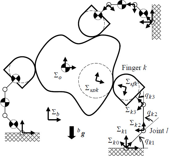
3.1. Joint Position and Local Coordinate Frame

The pose of the local contact frame ${\Sigma }_{Lok}$ with respect to ${\Sigma }_b$ is represented by

$${}^{b}A_{Lok}({\mathit{\epsilon }}_o)={}^{b}A_{bo}{}^{bo}A_o({\mathit{\epsilon }}_o){}^{o}A_{Lok},{}^{bo}A_o({\mathit{\epsilon }}_o)=A_t({\mathit{x}}_o)A_r({\zeta }_o),$$

(2)

where the vector ${\mathit{\epsilon }}_o={[{\mathit{x}}_o^T,{\zeta }_o]}^T$ is the object pose displacement, the vector ${\mathit{x}}_o={[x_o,y_o]}^T$ is translational component, and the scalar ${\zeta }_o$ is rotational component. The pose of the local contact frame ${\Sigma }_{Lfk}$ with respect to ${\Sigma }_b$ is represented by

$${}^{b}A_{Lfk}({\mathit{q}}_{dk})={}^{b}A_{k0}{}^{k0}A_{k1}(q_{dk1}){}^{k1}A_{k2}(q_{dk2}){}^{k2}A_{k3}(q_{dk3}){}^{k3}A_{Lfk},$$

(3)

where ${\mathit{q}}_{dk}={[q_{dk1},q_{dk2},q_{dk3}]}^T$ is the joint position displacement vector generated by ${\mathit{\epsilon }}_o$. The frame ${\Sigma }_{kl}$ is fixed in the l-th link of the finger. In the case of revolute joint, the matrix is represented by

$${}^{k,l-1}A_{kl}(q_{dkl})={}^{k,l-1}A_{bkl}(q_{nkl}+q_{ckl})A_r(q_{dkl}),$$

(4)

where $q_{nkl}$ and $q_{ckl}$ are the natural length and the initial compression of the spring, respectively. In the case of prismatic joint, the matrix is represented by

$${}^{k,l-1}A_{kl}(q_{dkl})={}^{k,l-1}A_{bkl}(q_{nkl}+q_{ckl})A_t(q_{dkl}{\mathit{u}}_1).$$

(5)

The frame ${\Sigma }_{bkl}$ is the initial frame of ${\Sigma }_{kl}$. The link shape is included in the matrix ${}^{k,l-1}A_{bkl}$. The joint position $q_{kl}$ shown in Figure 1 is given by $q_{kl}:=q_{nkl}+q_{ckl}+q_{dkl}$. The parameter $q_{dkl}$ is separated from $q_{nkl}$ and $q_{ckl}$ because $q_{dkl}$ is most important for our derivations. From these definitions, we have the following partial derivative (See Appendix A of [22]):

$$\frac{\partial {}^{k,l-1}A_{kl}(q_{dkl})}{\partial q_{dkl}}={}^{k,l-1}A_{kl}(q_{dkl})\left[\begin{array}{cc}{\omega }_{kl}\Omega & v_{kl}{u}_1\\ 0_{1\times 2}& 0\end{array}\right],\{\begin{array}{ccc}{\omega }_{kl}=1,& v_{kl}=0,& \text{for revolute joint}\\ {\omega }_{kl}=0,& v_{kl}=1,& \text{for prismatic joint}\end{array}.$$

(6)

3.2. Potential Energy of the Finger

The potential energy stored in the joint springs is represented by

$$U_{sk}({\mathit{q}}_{dk}):=\frac{1}{2}{[{\mathit{q}}_{ck}+{\mathit{q}}_{dk}]}^T{S}_k[{\mathit{q}}_{ck}+{\mathit{q}}_{dk}],$$

(7)

where the vector ${\mathit{q}}_{ck}={[q_{ck1},q_{ck2},q_{ck3}]}^T$ denotes the joint compression and the matrix $S_k\in {\text{R}}^{3\times 3}$ is joint stiffness. The joint torque vector is given by ${\mathit{\tau }}_{sk}:=S_k{\mathit{q}}_{ck}$. The potential energy affected by the gravity is represented by

$$U_{gk}({\mathit{q}}_{dk}):=-{\displaystyle \sum _{l=1}^3{m}_{kl}{}^b\mathit{p}_{gkl}^T({\mathit{q}}_{dk}){}^{b}g},$$

(8)

where $m_{kl}$ is the mass of the l-th link, the vector ${}^b\mathit{g}$ is the gravity acceleration with respect to the frame ${\Sigma }_b$, the frame ${\Sigma }_{gkl}$ is the center of the link mass.

$${}^b\mathit{p}_{gkl}=I_{23}{}^{b}A_{gkl}({\mathit{q}}_{dk}){\mathit{v}}_{\zeta },{}^{b}A_{gkl}({\mathit{q}}_{dk}):={}^{b}A_{k0}{}^{k0}A_{k1}(q_{dk1})\times \cdots \times {}^{k,l-1}A_{kl}(q_{dkl}){}^{kl}A_{gkl}.$$

(9)

The total potential energy of the finger is given by

$$U_k({\mathit{q}}_{dk}):=U_{sk}({\mathit{q}}_{dk})+U_{gk}({\mathit{q}}_{dk}).$$

(10)

The first- and second-order partial derivatives of $U_{gk}({\mathit{q}}_{dk})$ with respect to the joint positions are given by

$${\mathit{\tau }}_{gk}:={\frac{\partial U_{gk}(q_{dk})}{\partial q_{dk}}|}_0,S_{gk}:={\frac{{\partial }^2{U}_{gk}(q_{dk})}{\partial q_{dk}\partial q_{dk}^T}|}_0.$$

(11)

These detailed derivations are described in Appendix A. The vector ${\mathit{\tau }}_{gk}$ and the matrix $S_{gk}$ depend on the parameter $m_{kl}$, ${}^{b}A_{kl}$, and ${}^{kl}A_{gkl}$. In this paper, the right side symbol “${|}_0$” means that the initial condition is considered for the differentiations (${\mathit{\epsilon }}_o$ =0, ${\mathit{\alpha }}_k$ =0, ${\mathit{q}}_{dk}$ =0).

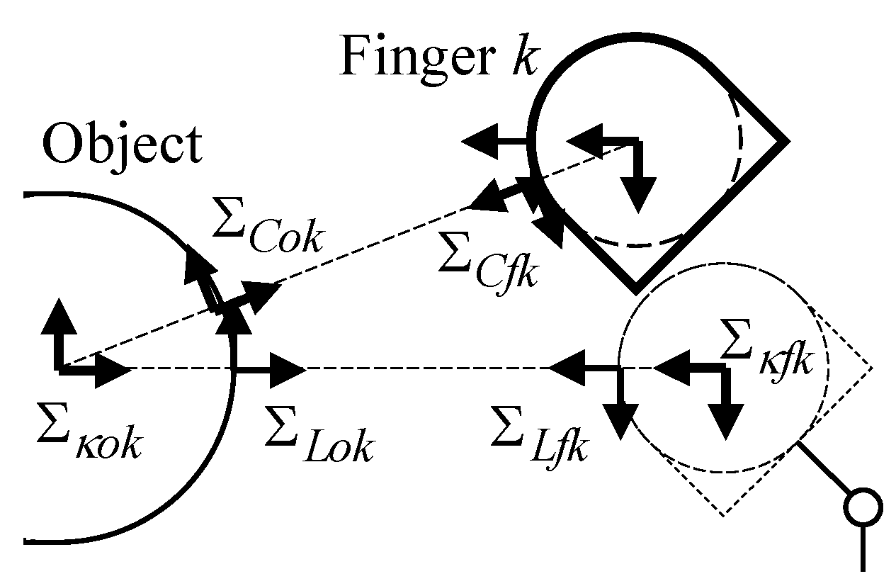
3.3. Contact Constraint and Its Partial Derivative

The pose of the current contact frame ${\Sigma }_{Cok}$ with respect to ${\Sigma }_b$ is represented by the following form:

$${}^{b}A_{Lfk}({\mathit{q}}_{dk}){}^{Lfk}A_{Cfk}({\mathit{\alpha }}_{fk}){}^{Cfk}A_{Cok}={}^{b}A_{Lok}({\mathit{\epsilon }}_o){}^{Lok}A_{Cok}({\mathit{\alpha }}_{ok}),$$

(12)

where ${}^{Cfk}A_{Cok}=A_r(\pi )$. From Equation (12), the vector ${\mathit{q}}_{dk}$ is given by a function of ${\mathit{\epsilon }}_o$ and ${\mathit{\alpha }}_k:={[{\mathit{\alpha }}_{ok},{\mathit{\alpha }}_{fk}]}^T$, i.e., ${\mathit{q}}_{dk}({\mathit{\epsilon }}_o,{\mathit{\alpha }}_k)$. The first-order partial derivative of Equation (12) is given by

$${}^{Lfk}J\left[\begin{array}{cc}{\frac{\partial q_{dk}}{\partial {\mathit{\epsilon }}_o^T}|}_0& {\frac{\partial q_{dk}}{\partial {\mathit{\alpha }}_k^T}|}_0\end{array}\right]=\left[\begin{array}{ccc}{}^{Lfk}B_o& \begin{array}{c}-{\mathit{u}}_2\\ {\kappa }_{ok}\end{array}& \begin{array}{c}-{\mathit{u}}_2\\ -{\kappa }_{fk}\end{array}\end{array}\right],$$

(13)

where

$${}^{Lfk}J:=\left[\begin{array}{ccc}{}^{Lfk}B_{k1}\left[\begin{array}{c}{v}_{k1}{\mathit{u}}_1\\ {\omega }_{k1}\end{array}\right]& {}^{Lfk}B_{k2}\left[\begin{array}{c}{v}_{k2}{\mathit{u}}_1\\ {\omega }_{k2}\end{array}\right]& {}^{Lfk}B_{k3}\left[\begin{array}{c}{v}_{k3}{\mathit{u}}_1\\ {\omega }_{k3}\end{array}\right]\end{array}\right]\in {\text{R}}^{3\times 3}.$$

(14)

The matrix ${}^{Lfk}J$ depends on ${}^{kl}A_{Lfk}$. The second-order partial derivative is shown in Appendix B. The quantities ${\kappa }_{ok}$ and ${\kappa }_{fk}$ are the local curvatures at contact points on the object and the finger, respectively. The quantity $\kappa$ is positive, zero, and negative if the surface shape is convex, flat, and concave, respectively.

3.4. Partial Derivatives of the Energy

From Equations (10) and (12), the potential energy is represented by

$$U_k({\mathit{q}}_{dk}({\mathit{\epsilon }}_o,{\mathit{\alpha }}_k))=U_{sk}({\mathit{q}}_{dk}({\mathit{\epsilon }}_o,{\mathit{\alpha }}_k))+U_{gk}({\mathit{q}}_{dk}({\mathit{\epsilon }}_o,{\mathit{\alpha }}_k)).$$

(15)

The first-order partial derivative of the energy with respect to ${\mathit{\epsilon }}_o$ and ${\mathit{\alpha }}_k$ is given by

$$\left[\begin{array}{c}{U}_{k,\mathit{\epsilon }}\\ U_{k,\mathit{\alpha }}\end{array}\right]:=\left[\begin{array}{c}{\frac{\partial U_k({\mathit{\epsilon }}_o,{\mathit{\alpha }}_k)}{\partial {\mathit{\epsilon }}_o}|}_0\\ {\frac{\partial U_k({\mathit{\epsilon }}_o,{\mathit{\alpha }}_k)}{\partial {\mathit{\alpha }}_k}|}_0\end{array}\right]=\left[\begin{array}{c}{\frac{\partial \{q_{dk}^T({\mathit{\epsilon }}_o,{\mathit{\alpha }}_k){\mathit{\tau }}_{Lfk}\}}{\partial {\mathit{\epsilon }}_o}|}_0\\ {\frac{\partial \{q_{dk}^T({\mathit{\epsilon }}_o,{\mathit{\alpha }}_k){\mathit{\tau }}_{Lfk}\}}{\partial {\mathit{\alpha }}_k}|}_0\end{array}\right]=\left[\begin{array}{c}{}^{Lfk}B_o^T\\ \begin{array}{cc}-{\mathit{u}}_2^T& {\kappa }_{ok}\\ -{\mathit{u}}_2^T& -{\kappa }_{fk}\end{array}\end{array}\right]{}^{Lfk}\mathit{w},$$

(16)

where the vector ${}^{Lfk}\mathit{w}$ means the wrench (force and moment) vector represented at the local contact frame ${\Sigma }_{Lfk}$. Note that this wrench vector is given as the reaction force from the object to the finger because ${\mathit{q}}_{ck}$ is compression.

$${}^{Lfk}\mathit{w}=\left[\begin{array}{c}{}^{Lfk}\mathit{f}\\ {}^{Lfk}n\end{array}\right]=\left[\begin{array}{c}{}^{Lfk}f_x\\ {}^{Lfk}f_y\\ {}^{Lfk}n\end{array}\right]:={}^{Lfk}J^{-T}{\mathit{\tau }}_{Lfk},{\mathit{\tau }}_{Lfk}={\mathit{\tau }}_{sk}+{\mathit{\tau }}_{gk}.$$

(17)

The detailed derivations are described in Appendix B. The second-order partial derivative is given by

$$\left[\begin{array}{cc}{U}_{k,\mathit{\epsilon }\mathit{\epsilon }}& U_{k,\mathit{\alpha }\mathit{\epsilon }}\\ U_{k,\mathit{\epsilon }\mathit{\alpha }}& U_{k,\mathit{\alpha }\mathit{\alpha }}\end{array}\right]:=\left[\begin{array}{cc}{\frac{{\partial }^2{U}_k({\mathit{\epsilon }}_o,{\mathit{\alpha }}_k)}{\partial {\mathit{\epsilon }}_o\partial {\mathit{\epsilon }}_o^T}|}_0& {\frac{{\partial }^2{U}_k({\mathit{\epsilon }}_o,{\mathit{\alpha }}_k)}{\partial {\mathit{\epsilon }}_o\partial {\mathit{\alpha }}_k^T}|}_0\\ {\frac{{\partial }^2{U}_k({\mathit{\epsilon }}_o,{\mathit{\alpha }}_k)}{\partial {\mathit{\alpha }}_k\partial {\mathit{\epsilon }}_o^T}|}_0& {\frac{{\partial }^2{U}_k({\mathit{\epsilon }}_o,{\mathit{\alpha }}_k)}{\partial {\mathit{\alpha }}_k\partial {\mathit{\alpha }}_k^T}|}_0\end{array}\right]=\left[\begin{array}{c}{\frac{\partial q_{dk}^T({\mathit{\epsilon }}_o,{\mathit{\alpha }}_k)}{\partial {\mathit{\epsilon }}_o}|}_0\\ {\frac{\partial q_{dk}^T({\mathit{\epsilon }}_o,{\mathit{\alpha }}_k)}{\partial {\mathit{\alpha }}_k}|}_0\end{array}\right][S_k+S_{gk}]{\left[\begin{array}{c}{\frac{\partial q_{dk}^T({\mathit{\epsilon }}_o,{\mathit{\alpha }}_k)}{\partial {\mathit{\epsilon }}_o}|}_0\\ {\frac{\partial q_{dk}^T({\mathit{\epsilon }}_o,{\mathit{\alpha }}_k)}{\partial {\mathit{\alpha }}_k}|}_0\end{array}\right]}^T+\left[\begin{array}{cc}{\frac{{\partial }^2\{{\mathit{\tau }}_{Lfk}^T{q}_{dk}({\mathit{\epsilon }}_o,{\mathit{\alpha }}_k)\}}{\partial {\mathit{\epsilon }}_o\partial {\mathit{\epsilon }}_o^T}|}_0& {\frac{{\partial }^2\{{\mathit{\tau }}_{Lfk}^T{q}_{dk}({\mathit{\epsilon }}_o,{\mathit{\alpha }}_k)\}}{\partial {\mathit{\epsilon }}_o\partial {\mathit{\alpha }}_k^T}|}_0\\ {\frac{{\partial }^2\{{\mathit{\tau }}_{Lfk}^T{q}_{dk}({\mathit{\epsilon }}_o,{\mathit{\alpha }}_k)\}}{\partial {\mathit{\alpha }}_k\partial {\mathit{\epsilon }}_o^T}|}_0& {\frac{{\partial }^2\{{\mathit{\tau }}_{Lfk}^T{q}_{dk}({\mathit{\epsilon }}_o,{\mathit{\alpha }}_k)\}}{\partial {\mathit{\alpha }}_k\partial {\mathit{\alpha }}_k^T}|}_0\end{array}\right]=\left[\begin{array}{c}{}^{Lfk}B_o^T\\ \begin{array}{cc}-{\mathit{u}}_2^T& {\kappa }_{ok}\\ -{\mathit{u}}_2^T& -{\kappa }_{fk}\end{array}\end{array}\right]{}^{Lfk}S{\left[\begin{array}{c}{}^{Lfk}B_o^T\\ \begin{array}{cc}-{\mathit{u}}_2^T& {\kappa }_{ok}\\ -{\mathit{u}}_2^T& -{\kappa }_{fk}\end{array}\end{array}\right]}^T+\left[\begin{array}{cc}{v}_{\zeta }& 0_{3\times 2}\\ 0_{2\times 1}& I_2\end{array}\right]S_{\kappa k}{\left[\begin{array}{cc}{v}_{\zeta }& 0_{3\times 2}\\ 0_{2\times 1}& I_2\end{array}\right]}^T,$$

(18)

where

$${}^{Lfk}S:={}^{Lfk}J^{-T}[S_k+S_{gk}+S_{Lfk}]{}^{Lfk}J^{-1}.$$

(19)

The detailed derivations of the matrices $S_{Lfk}$ and $S_{\kappa k}$ are shown in Appendix B. The matrix $S_{Lfk}$ depends on ${}^{kl}A_{Lfk}$ and ${}^{Lfk}\mathit{f}$, and the matrix $S_{\kappa k}$ depends on ${}^{o}A_{Lfk}$, ${\kappa }_{ok}$, ${\kappa }_{fk}$, and ${}^{Lfk}\mathit{f}$.

Summarizing the above derivations, we have the following terms:

$$U_{k,\mathit{\epsilon }}={}^{Lfk}B_o^T{}^{Lfk}\mathit{w},U_{k,\mathit{\alpha }}=\left[\begin{array}{cc}-u_2^T& {\kappa }_{ok}\\ -u_2^T& -{\kappa }_{fk}\end{array}\right]{}^{Lfk}\mathit{w},U_{k,\mathit{\epsilon }\mathit{\epsilon }}={}^{Lfk}B_o^T{}^{Lfk}S{}^{Lfk}B_o+[{}^{Lfk}\mathit{p}_o^T{}^{Lfk}\mathit{f}]{\mathit{v}}_{\zeta }{\mathit{v}}_{\zeta }^T,U_{k,\mathit{\alpha }\mathit{\epsilon }}=U_{k,\mathit{\epsilon }\mathit{\alpha }}^T={}^{Lfk}B_o^T{}^{Lfk}S\left[\begin{array}{cc}-u_2& -u_2\\ {\kappa }_{ok}& -{\kappa }_{fk}\end{array}\right]+[{\mathit{u}}_1^T{}^{Lfk}\mathit{f}]{\mathit{v}}_{\zeta }[\begin{array}{cc}1& 1\end{array}],U_{k,\mathit{\alpha }\mathit{\alpha }}={\left[\begin{array}{cc}-u_2& -u_2\\ {\kappa }_{ok}& -{\kappa }_{fk}\end{array}\right]}^T{}^{Lfk}S\left[\begin{array}{cc}-u_2& -u_2\\ {\kappa }_{ok}& -{\kappa }_{fk}\end{array}\right]+[{\mathit{u}}_1^T{}^{Lfk}\mathit{f}]\left[\begin{array}{cc}{\kappa }_{ok}& {\kappa }_{ok}\\ {\kappa }_{ok}& -{\kappa }_{fk}\end{array}\right].$$

(20)

3.5. Frictionless Sliding Contact Case

3.5.1. Wrench Vector and Stiffness Matrix

In the case of frictionless sliding contact, the contact displacement parameter ${\mathit{\alpha }}_k$ has to satisfy the following conditions:

$$\frac{\partial U_k({\mathit{\epsilon }}_o,{\mathit{\alpha }}_k)}{\partial {\mathit{\alpha }}_k}=0_{2\times 1},\frac{{\partial }^2{U}_k({\mathit{\epsilon }}_o,{\mathit{\alpha }}_k)}{\partial {\mathit{\alpha }}_k\partial {\mathit{\alpha }}_k^T}>0_{2\times 2}.$$

(21)

Under the initial condition of Equation (21), we have $U_{k,\mathit{\alpha }}=0_{2\times 1}$ and then ${}^{Lfk}f_y=0$ and ${}^{Lfk}n=0$. Hence, the contact wrench is represented by

$${}^{Lfk}\mathit{w}={}^{Lfk}f_x{[1,0,0]}^T.$$

(22)

Because the finger can apply pushing forces to the object, we have ${}^{Lfk}f_x={\mathit{u}}_1^T{}^{Lfk}\mathit{f}<0$. Note that the x axis direction of ${\Sigma }_{Lfk}$ is opposite to the reaction force direction. We have also $U_{k,\mathit{\alpha }\mathit{\alpha }}>0_{2\times 2}$>. This inequality means that positive stiffness has to be generated in the displacement direction ${\mathit{\alpha }}_k$.

From the first condition of Equation (21), the parameter ${\mathit{\alpha }}_k$> is given by a function of the parameter ${\mathit{\epsilon }}_o$.

$$U_k^{fs}({\mathit{\epsilon }}_o):=U_k({\mathit{\epsilon }}_o,{\mathit{\alpha }}_k^{fs}({\mathit{\epsilon }}_o)),$$

(23)

where the superscript “fs” means the sliding contact between the finger and the object. The wrench vector generated at the object coordinate frame is given by

$$G_k^{fs}:={\frac{\partial U_k^{fs}({\mathit{\epsilon }}_o)}{\partial {\mathit{\epsilon }}_o}|}_0={}^{o}W_{Lfk}[{}^{Lfk}f_x{\mathit{u}}_1].$$

(24)

The stiffness matrix of the sliding contact is given by

$$H_k^{fs}:={\frac{{\partial }^2{U}_k^{fs}({\mathit{\epsilon }}_o)}{\partial {\mathit{\epsilon }}_o\partial {\mathit{\epsilon }}_o^T}|}_0=U_{k,\mathit{\epsilon }\mathit{\epsilon }}+Q_k^{fs}{U}_{k,\mathit{\epsilon }\mathit{\alpha }},$$

(25)

where

$$Q_k^{fs}:={\frac{\partial {[{\mathit{\alpha }}_k^{fs}({\mathit{\epsilon }}_o)]}^T}{\partial {\mathit{\epsilon }}_o}|}_0=-U_{k,\mathit{\alpha }\mathit{\epsilon }}{U}_{k,\mathit{\alpha }\mathit{\alpha }}^{-1}.$$

(26)

The symbols G and H mean the gradient and the Hessian of the energy. These derivations are described in Appendix C.

3.5.2. Local Curvature Effect

The wrench vector and the stiffness matrix are given by functions of grasp parameters. The partial derivatives of the vector and the matrix with respect to the local curvature parameters are given by

$$\frac{\partial G_k^{fs}}{\partial {\kappa }_{ok}}=\frac{\partial G_k^{fs}}{\partial {\kappa }_{fk}}=0_{3\times 1}.$$

(27)

This means that the wrench vector is independent of the local curvatures.

$$\frac{\partial H_k^{fs}}{\partial {\kappa }_{ok}}={}^{Lfk}f_x[Q_k^{fs}{\mathit{u}}_1]{[Q_k^{fs}{u}_1]}^T\le 0_{3\times 3},\frac{\partial H_k^{fs}}{\partial {\kappa }_{fk}}={}^{Lfk}f_x[Q_k^{fs}{\mathit{u}}_2]{[Q_k^{fs}{u}_2]}^T\le 0_{3\times 3}.$$

(28)

The properties of these negative semi-definite matrices imply that the grasp stability decreases when the local curvature parameters increase. The effects are given in the directions $Q_k^{fs}{\mathit{u}}_1$ and $Q_k^{fs}{\mathit{u}}_2$ when the local curvatures ${\kappa }_{ok}$ and ${\kappa }_{fk}$ deviate, respectively.

3.6. Pure Rolling Contact Case

3.6.1. Wrench Vector and Stiffness Matrix

In the case of a pure rolling contact, we have ${\mathit{\alpha }}_{ok}+{\mathit{\alpha }}_{fk}=0$. The potential energy is represented by

$$U_k^r({\mathit{\epsilon }}_o,{\mathit{\alpha }}_{ok}):=U_k({\mathit{\epsilon }}_o,{\mathit{\alpha }}_{ok},-{\mathit{\alpha }}_{ok}).$$

(29)

In the case of pure rolling contact, the contact position displacement ${\mathit{\alpha }}_{ok}$ has to satisfy the following conditions

$$\frac{\partial U_k^r({\mathit{\epsilon }}_o,{\mathit{\alpha }}_{ok})}{\partial {\mathit{\alpha }}_{ok}}=0,\frac{{\partial }^2{U}_k^r({\mathit{\epsilon }}_o,{\mathit{\alpha }}_{ok})}{\partial {\mathit{\alpha }}_{ok}\partial {\mathit{\alpha }}_{ok}}>0.$$

(30)

At the initial condition of Equation (30), we have $U_{k,\mathit{\alpha }}^r=0$ and then ${}^{Lfk}n=0$. We have also $U_{k,\mathit{\alpha }\mathit{\alpha }}^r>0$. This means that a positive stiffness has to be generated in the displacement direction ${\mathit{\alpha }}_{ok}$.

From the first condition of Equation (30), the parameter ${\mathit{\alpha }}_{ok}$ is given by a function of ${\mathit{\epsilon }}_o$.

$$U_k^{fr}({\mathit{\epsilon }}_o):=U_k^r({\mathit{\epsilon }}_o,{\mathit{\alpha }}_{ok}^{fr}({\mathit{\epsilon }}_o)),$$

(31)

where the superscript “fr” means the rolling contact between the finger and the object. The wrench vector at the contact point is given by

$$G_k^{fr}:={\frac{\partial U_k^{fr}({\mathit{\epsilon }}_o)}{\partial {\mathit{\epsilon }}_o}|}_0={}^{o}W_{Lfk}{}^{Lfk}\mathit{f}.$$

(32)

The stiffness matrix of the pure rolling contact is given by

$$H_k^{fr}:={\frac{{\partial }^2{U}_k^{fr}({\mathit{\epsilon }}_o)}{\partial {\mathit{\epsilon }}_o\partial {\mathit{\epsilon }}_o^T}|}_0=U_{k,\mathit{\epsilon }\mathit{\epsilon }}^r+Q_k^{fr}{U}_{k,\mathit{\epsilon }\mathit{\alpha }}^r.$$

(33)

where

$$Q_k^{fr}:={\frac{\partial {\mathit{\alpha }}_{ok}^{fr}({\mathit{\epsilon }}_o)}{\partial {\mathit{\epsilon }}_o}|}_0=-U_{k,\mathit{\alpha }\mathit{\epsilon }}^r{[U_{k,\mathit{\alpha }\mathit{\alpha }}^r]}^{-1}.$$

(34)

These derivations are described in Appendix D.

3.6.2. Local Curvature Effect

The partial derivatives of the wrench vector and the stiffness matrix by the local curvature parameters are given by

$$\frac{\partial G_k^{fr}}{\partial {\kappa }_{ok}}=\frac{\partial G_k^{fr}}{\partial {\kappa }_{fk}}=0_{3\times 1}.$$

(35)

This means that the wrench vector is independent of the local curvatures.

$$\frac{\partial H_k^{fr}}{\partial {\kappa }_{ok}}=\frac{\partial H_k^{fr}}{\partial {\kappa }_{fk}}={}^{Lfk}f_x{Q}_k^{fr}{[Q_k^{fr}]}^T\le 0_{3\times 3}.$$

(36)

The properties of these negative semi-definite matrices imply that the grasp stability decreases when the local curvature parameters increase. The effect of the local curvature deviation appears in the direction $Q_k^{fr}$. These derivations are described in Appendix D.

3.7. Contact Condition Effect

To compare the stiffness matrices of the pure rolling contact and the frictionless sliding contact in the same force condition, we assume $U_{k,\mathit{\alpha }}=0_{2\times 1}$. The difference matrix is given by

$$H_k^{fd}:=H_k^{fr}-H_k^{fs}=U_{k,\mathit{\alpha }\mathit{\epsilon }}{U}_{k,\mathit{\alpha }\mathit{\alpha }}^{-1}{U}_{k,\mathit{\epsilon }\mathit{\alpha }}-[U_{k,\mathit{\alpha }\mathit{\epsilon }}\mathit{z}]{[z^T{U}_{k,\mathit{\alpha }\mathit{\alpha }}z]}^{-1}{[U_{k,\mathit{\alpha }\mathit{\epsilon }}z]}^T=\frac{U_{k,\mathit{\alpha }\mathit{\epsilon }}{U}_{k,\mathit{\alpha }\mathit{\alpha }}^{-1}\{[z^T{U}_{k,\mathit{\alpha }\mathit{\alpha }}z]U_{k,\mathit{\alpha }\mathit{\alpha }}-U_{k,\mathit{\alpha }\mathit{\alpha }}z{z}^T{U}_{k,\mathit{\alpha }\mathit{\alpha }}\}{U}_{k,\mathit{\alpha }\mathit{\alpha }}^{-1}{U}_{k,\mathit{\epsilon }\mathit{\alpha }}}{z^T{U}_{k,\mathit{\alpha }\mathit{\alpha }}z}=\frac{\left|U_{k,\mathit{\alpha }\mathit{\alpha }}\right|}{U_{k,\mathit{\alpha }\mathit{\alpha }}^r}\left\{Q_k^{fs}\left[\begin{array}{c}1\\ 1\end{array}\right]\right\}{\left\{Q_k^{fs}\left[\begin{array}{c}1\\ 1\end{array}\right]\right\}}^T>0_{3\times 3}.$$

(37)

It is shown that the pure rolling contact is more stable than the frictionless sliding contact because $H_k^{fd}$ is a positive definite matrix. The effect of the contact condition difference appears in the direction $Q_k^{fs}{[1,1]}^T$.

3.8. Grasp Wrench and Stiffness Matrix

The total potential energy of the grasp is given by

$$U({\mathit{\epsilon }}_o)=U_{go}({\mathit{\epsilon }}_o)+{\displaystyle \sum _k{U}_k^{fc}({\mathit{\epsilon }}_o),}$$

(38)

where the superscript “fc” is “fs” for the sliding contact or “fr” for the rolling contact. The symbol $U_{go}({\mathit{\epsilon }}_o)$ is the potential energy of the object affected by the gravity.

$$U_{go}({\mathit{\epsilon }}_o):=-m_o{}^b\mathit{p}_{go}^T({\mathit{\epsilon }}_o){}^b\mathit{g},{}^b\mathit{p}_{go}({\mathit{\epsilon }}_o)=I_{23}{}^{b}A_{bo}{}^{bo}A_o({\mathit{\epsilon }}_o){}^{o}A_{go}{\mathit{v}}_{\zeta },$$

(39)

The frame ${\Sigma }_{go}$ represents the center of the object mass.

The wrench vector and the stiffness matrix of the grasp are given by

$$G:={\frac{\partial U({\mathit{\epsilon }}_o)}{\partial {\mathit{\epsilon }}_o}|}_0=G_{go}+{\displaystyle \sum _k{G}_k^{fc}},H:={\frac{{\partial }^{2}U({\mathit{\epsilon }}_o)}{\partial {\mathit{\epsilon }}_o\partial {\mathit{\epsilon }}_o^T}|}_0=H_{go}+{\displaystyle \sum _k{H}_k^{fc}.}$$

(40)

The grasp stability is evaluated by the eigenvalues of the matrix H when the wrench vector G is zero (wrench equilibrium). The wrench vector and the grasp stiffness matrix are represented in the object frame ${\Sigma }_{bo}$.

4. Numerical Examples

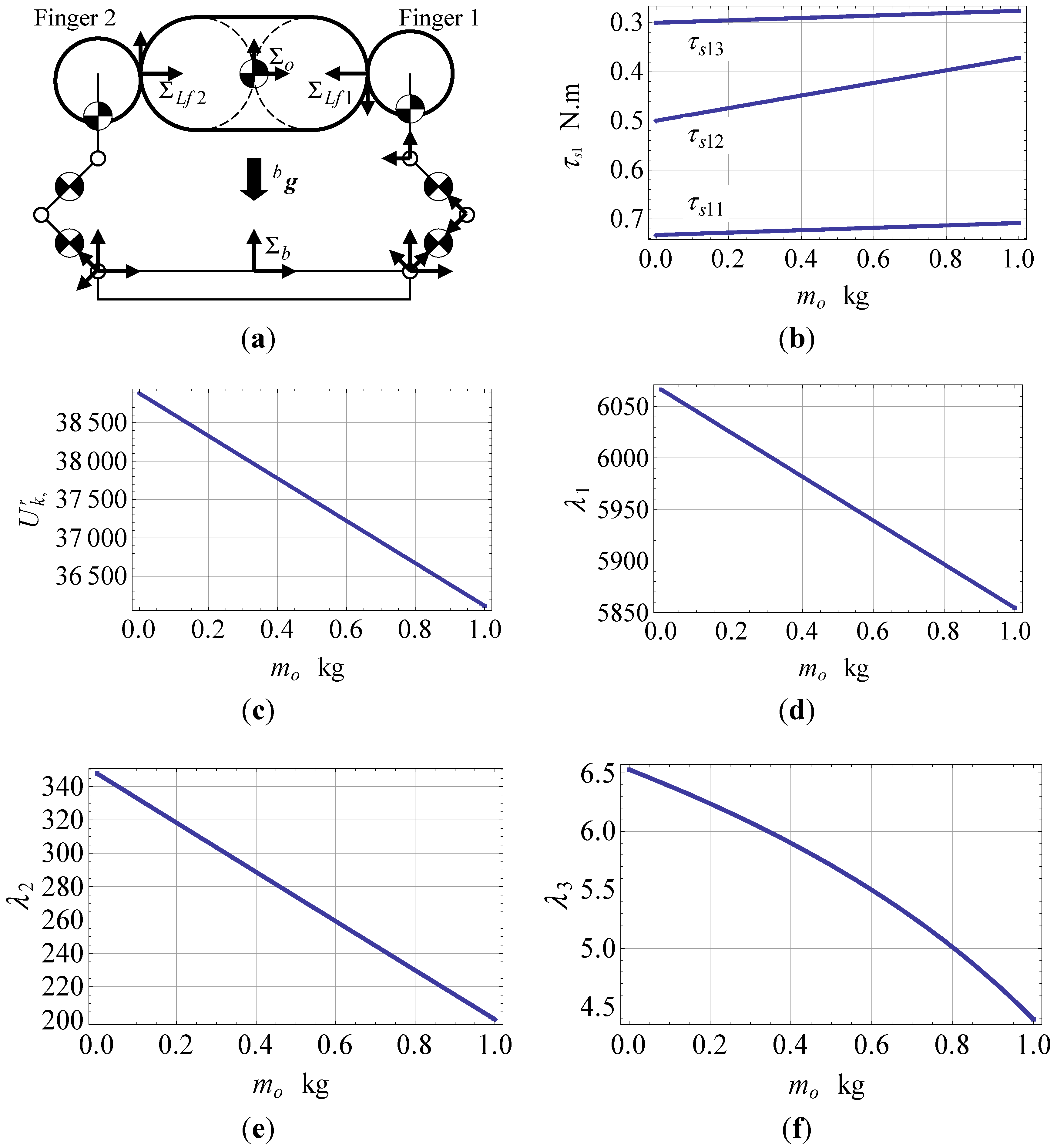
We show examples in order to demonstrate the effectiveness of our analysis. In our method, the number of fingers and the shape of the object and fingers are not limited if ${\kappa }_{ok}+{\kappa }_{fk}>0$. In order for the reader to easily understand our analysis, we show simple examples. Because the effects of the local curvatures have been analytically derived as shown in Equations (28) and (36), we omit the explanations on the curvature effects in this section.

4.1. Example 1

Assume the case of an object grasped by two fingers with three revolute joints. The object is grasped in the palm of the hand. The shape of the fingers and the object is shown in Figure 3. The physical parameters are set as shown in Table 2.

Figure 3. Grasp example 1. (a) An object grasped by two fingers. (b) Contact force direction. (c) Contact force ${}^{Lf1}\mathit{f}$. (d) Joint torque ${\mathit{\tau }}_{s1}$. (e) Finger stability condition $U_{k,\mathit{\alpha }\mathit{\alpha }}^r$. (f) Eigenvalue ${\lambda }_1$. (g) Eigenvalue ${\lambda }_2$. (h) Eigenvalue.

Figure 3. Grasp example 1. (a) An object grasped by two fingers. (b) Contact force direction. (c) Contact force ${}^{Lf1}\mathit{f}$. (d) Joint torque ${\mathit{\tau }}_{s1}$. (e) Finger stability condition $U_{k,\mathit{\alpha }\mathit{\alpha }}^r$. (f) Eigenvalue ${\lambda }_1$. (g) Eigenvalue ${\lambda }_2$. (h) Eigenvalue.

Table 2. Physical Parameters.

Gravity acceleration	g = 9.8 (m/s2)
Gravity acceleration vector	bg = $-g{u}_2$
Mass of the object	mo
Mass of the link	mkl = 0.04 (kg)
Object half length	lo = 0.02 (m)
Finger link length	lkl = 0.03 (m)
Local curvature of the object	κok = 100 (1/m)
Local curvature of the finger	κfk = 200 (1/m)
Joint stiffness matrix	Sk = diag[1,1,1] (N∙m/rad)
Joint angles of the finger 1	(q11, q12, q13) = ($\pi /4$, $\pi /4$, $\pi /4$) (rad)
Joint angles of the finger 2	(q21, q22, q23) = ($3\pi /4$, $-\pi /4$, $-\pi /4$) (rad)
Directions of the contact points	(θ1, θ2) = ($\pi /4$, $-\pi /4$) (rad)
Center of the object mass	${}^{o}A_{go}=I_3$
Local contact frames on the object	${}^{o}A_{Lo1}=A_t(l_o{u}_1)$, ${}^{o}A_{Lo2}(\pi ){}^{o}A_{Lo1}$
Frames of the finger	${}^{k0}A_{k1}=A_r(q_{k1})$, ${}^{k1}A_{k2}=A_t(l_{k1}{u}_1)A_r(q_{k2})$, ${}^{k2}A_{k3}=A_t(l_{k2}{u}_1)A_r(q_{k3})$, ${}^{k3}A_{Lfk}=A_t(l_{k3}{u}_1)A_r({\theta }_k)A_t({\kappa }_{fk}^{-1}{u}_1)$
Finger base frames	${}^{b}A_{10}=A_t((l_o+{\kappa }_{fk}^{-1})u_1)$, ${}^{b}A_{20}=A_t(-(l_o+{\kappa }_{fk}^{-1})u_1)$
Center of the link mass	${}^{kl}A_{gkl}=A_t((l_{kl}/2)u_1)$
Contact force	f := $-{}^{Lfk}f_x$ = 10 (N)

Table 2. Physical Parameters.

Gravity acceleration	g = 9.8 (m/s2)
Gravity acceleration vector	bg = $-g{u}_2$
Mass of the object	mo
Mass of the link	mkl = 0.04 (kg)
Object half length	lo = 0.02 (m)
Finger link length	lkl = 0.03 (m)
Local curvature of the object	κok = 100 (1/m)
Local curvature of the finger	κfk = 200 (1/m)
Joint stiffness matrix	Sk = diag[1,1,1] (N∙m/rad)
Joint angles of the finger 1	(q11, q12, q13) = ($\pi /4$, $\pi /4$, $\pi /4$) (rad)
Joint angles of the finger 2	(q21, q22, q23) = ($3\pi /4$, $-\pi /4$, $-\pi /4$) (rad)
Directions of the contact points	(θ1, θ2) = ($\pi /4$, $-\pi /4$) (rad)
Center of the object mass	${}^{o}A_{go}=I_3$
Local contact frames on the object	${}^{o}A_{Lo1}=A_t(l_o{u}_1)$, ${}^{o}A_{Lo2}(\pi ){}^{o}A_{Lo1}$
Frames of the finger	${}^{k0}A_{k1}=A_r(q_{k1})$, ${}^{k1}A_{k2}=A_t(l_{k1}{u}_1)A_r(q_{k2})$, ${}^{k2}A_{k3}=A_t(l_{k2}{u}_1)A_r(q_{k3})$, ${}^{k3}A_{Lfk}=A_t(l_{k3}{u}_1)A_r({\theta }_k)A_t({\kappa }_{fk}^{-1}{u}_1)$
Finger base frames	${}^{b}A_{10}=A_t((l_o+{\kappa }_{fk}^{-1})u_1)$, ${}^{b}A_{20}=A_t(-(l_o+{\kappa }_{fk}^{-1})u_1)$
Center of the link mass	${}^{kl}A_{gkl}=A_t((l_{kl}/2)u_1)$
Contact force	f := $-{}^{Lfk}f_x$ = 10 (N)

We have $G_{go}=m_{o}g{[u_2^T,0]}^T$ and $H_{go}=0_{3\times 3}$. In order to generate the wrench equilibrium $G$ $=G_{go}+G_1^{fr}+G_2^{fr}$ $=0_{3\times 1}$, the contact forces are set to ${}^{Lf1}\mathit{f}$ = ${[-f,m_{o}g/2]}^T$ and ${}^{Lf2}\mathit{f}$ = ${[-f,-m_{o}g/2]}^T$. The component f means an internal force for preventing the slip between the object and the fingers. The y components generate forces to resist the object mass. The signs of the components depend on the relationship between the base frame ${\Sigma }_b$, the object frame ${\Sigma }_o$, and the contact frame ${\Sigma }_{Lfk}$ as shown in Figure 3b. In the case of the frictionless sliding contact, this grasp is infeasible because of ${\mathit{u}}_2^T{}^{Lfk}\mathit{f}\ne 0$. Hence, in this example, we show the results of the rolling contact case only.

Because of the revolute joints, we have ${\omega }_{kl}=1$ and $v_{kl}=0$, and then we obtain ${\mathit{\tau }}_{gk}$, $S_{gk}$, and $S_{Lfk}$. Figure 3c shows the contact force ${}^{Lf1}\mathit{f}$ in the case with f = 10 [N] with respect to the object mass m_o. From the above settings, the joint torque is obtained by

$${\mathit{\tau }}_{sk}={}^{Lfk}J^T{}^{Lfk}\mathit{w}-{\mathit{\tau }}_{gk}={}^{Lfk}J^T\left[\begin{array}{c}{}^{Lfk}\mathit{f}\\ 0\end{array}\right]-{\mathit{\tau }}_{gk}.$$

(41)

Figure 3d shows the joint torque ${\mathit{\tau }}_{s1}$. Similarly, ${\mathit{\tau }}_{s2}$ is obtained because of the bilateral symmetry grasp. From this figure, it is shown that the absolute values of the joint torques decrease when the object mass increases. In order to maintain the joint angles, the joint torques vary depending on the object mass.

$$\frac{\partial {\mathit{\tau }}_{s1}}{\partial m_o}=-\frac{\partial {\mathit{\tau }}_{s2}}{\partial m_o}=\frac{g}{2}{}^{Lf1}J^T\left[\begin{array}{c}0\\ 1\\ 0\end{array}\right]=-\frac{g}{2}\left[\begin{array}{c}{}^{Lf1}\mathit{p}_{11}^T{u}_1\\ {}^{Lf1}\mathit{p}_{12}^T{u}_1\\ {}^{Lf1}\mathit{p}_{13}^T{u}_1\end{array}\right].$$

(42)

In this example, we have ${}^{Lf1}\mathit{p}_{1l}^T{\mathit{u}}_1<0$, (l = 1, 2, 3) then the absolute values decrease as shown in Figure 3d. Figure 3e shows the finger stability condition $U_{k,\mathit{\alpha }\mathit{\alpha }}^r$. Because $U_{k,\mathit{\alpha }\mathit{\alpha }}^r$ is positive, the finger joint angles are stable. However, its margin decreases when the object mass increases because of

$$\frac{\partial U_{k,\mathit{\alpha }\mathit{\alpha }}^r}{\partial m_o}<0.$$

(43)

This partial derivative is described in Appendix E. The grasp stiffness matrix is given by

$$H=H_{go}+H_1^{fr}+H_2^{fr}=\left[\begin{array}{ccc}{h}_{11}& 0& h_{13}\\ 0& h_{22}& 0\\ h_{13}& 0& h_{33}\end{array}\right].$$

(44)

Because the elements of the matrix are complicated, they are omitted. The eigenvalues are obtained by

$${\lambda }_1=h_{22},\begin{array}{l}{\lambda }_2\\ {\lambda }_3\end{array}\}=\frac{(h_{11}+h_{33})\pm \sqrt{{(h_{11}-h_{33})}^2+4h_{13}^2}}{2}.$$

(45)

.

Figure 3f–h show the eigenvalues. The eigenvalue ${\lambda }_1$ is given in the y direction (vertical direction). The second eigenvalue is obtained mainly in the x direction (mainly horizontal direction). The third eigenvalue is obtained mainly in the rotation of the object. It is shown that the eigenvalues of the grasp stiffness matrix decrease when the object mass increases. This characteristic is obtained by the partial derivative of the matrix with respect to the object mass. From the derivation in Appendix E, we have the following negative definite matrix:

$$\frac{\partial H}{\partial m_o}<0_{3\times 3}.$$

(46)

This means that the eigenvalues decrease when the mass increases.

4.2. Example 2

We investigate the grasp shown in Figure 4a. Whereas the joint angles are the same as in Example 1, the direction of the gravity vector is opposite. This means that the object is grasped below the hand palm as shown in Figure 4a. Figure 4b shows the joint torques. In order to maintain the joint angles, the absolute values of the joint torques increase when the object mass increases. The required joint torque of this case is larger than that of Example 1. In Figure 4c, the finger stability condition increases when the mass increases. In Figure 4d–f, the eigenvalues of the grasp stiffness matrix also increase when the mass increases. Hence, the grasp stability increases when the mass increases. These results are obviously obtained from the following values:

$${}^{Lf1}\mathit{f}=\left[\begin{array}{c}-f\\ -\frac{m_{o}g}{2}\end{array}\right],{}^{Lf2}\mathit{f}=\left[\begin{array}{c}-f\\ \frac{m_{o}g}{2}\end{array}\right],\frac{\partial {\mathit{\tau }}_{s1}}{\partial m_o}=-\frac{\partial {\mathit{\tau }}_{s2}}{\partial m_o}=\frac{-g}{2}{}^{Lf1}J^T\left[\begin{array}{c}0\\ 1\\ 0\end{array}\right],\frac{\partial U_{k,\mathit{\alpha }\mathit{\alpha }}^r}{\partial m_o}>0,\frac{\partial H}{\partial m_o}>0_{3\times 3}.$$

(47)

This stability is similar to a pendulum system. Example 1 implies an inverse pendulum system.

Figure 4. Grasp example 2. (a) An object grasped under the palm. Joint torque ${\mathit{\tau }}_{s1}$. (c) Finger stability condition $U_{k,\mathit{\alpha }\mathit{\alpha }}^r$. (d) Eigenvalue ${\lambda }_1$. (e) Eigenvalue ${\lambda }_2$. (f) Eigenvalue ${\lambda }_3$.

Figure 4. Grasp example 2. (a) An object grasped under the palm. Joint torque ${\mathit{\tau }}_{s1}$. (c) Finger stability condition $U_{k,\mathit{\alpha }\mathit{\alpha }}^r$. (d) Eigenvalue ${\lambda }_1$. (e) Eigenvalue ${\lambda }_2$. (f) Eigenvalue ${\lambda }_3$.

4.3. Example 3

We investigate the grasp shown in Figure 5a. The gravity direction is the same as in Example 1, but the joint angles are different. The joint angles are set to (q₁₁, q₁₂, q₁₃) = ($\pi /2$, $-\pi /4$, $\pi /2$) and (q₂₁, q₂₂, q₂₃) = ($\pi /2$, $\pi /4$, $-\pi /2$). The directions of the contact points are the same as in Example 1. The absolute values of the joint torque decrease when the object mass increases (Figure 5b). The finger stability condition decreases and the eigenvalues of the grasp stiffness matrix decreases when the mass increases (Figure 5c–f). These characteristics are similarly obtained from the analysis of the partial derivative with respect to the object mass as described in Example 1. The margin of the finger stability condition is smaller than that of Example 1. The first and the second eigenvalues of this grasp are larger than those of Example 1, but the third eigenvalue is smaller than that of Example 1. This means that the rotational stability decreases while the translational stability increases as compared with Example 1.

Figure 5. Grasp case 3. (a) An object grasped by two fingers. (b) Joint torque ${\mathit{\tau }}_{s1}$. (c) Finger stability condition $U_{k,\mathit{\alpha }\mathit{\alpha }}^r$. (d) Eigenvalue. (e) Eigenvalue ${\lambda }_2$. (f) Eigenvalue ${\lambda }_3$

Figure 5. Grasp case 3. (a) An object grasped by two fingers. (b) Joint torque ${\mathit{\tau }}_{s1}$. (c) Finger stability condition $U_{k,\mathit{\alpha }\mathit{\alpha }}^r$. (d) Eigenvalue. (e) Eigenvalue ${\lambda }_2$. (f) Eigenvalue ${\lambda }_3$

4.4. Example 4

We investigate stability of the grasp shown in Figure 6a. Whereas the direction of the gravity is the same as in Examples 1 and 3, the joint angles and the contact points are different from the examples. In Figure 6a, the illustration of the fingertip shapes is somewhat different from the previous examples but the local curvatures at the contact points are the same as in the examples. The joint angles are set to (q₁₁, q₁₂, q₁₃) = ($\pi /4$, $\pi /2$, $-\pi /4$) and (q₂₁, q₂₂, q₂₃) = ($3\pi /4$, $-\pi /2$, $\pi /4$). The directions of the contact points are given to ${\theta }_1=\pi /2$ and ${\theta }_2=-\pi /2$. The absolute values of the joint torque decrease when the object mass increases (Figure 6b). The finger stability condition and the eigenvalues of the grasp stiffness matrix decrease (Figure 6c–f). The absolute values of the joint torques are larger than those of Example 1. The margin of the finger stability condition is smaller than that of Example 1 and larger than that of Example 3. The first and the third eigenvalues are smaller than those of Example 1.

Figure 6. Grasp case 4. (a) An object grasped by two fingers. (b) Joint torque ${\mathit{\tau }}_{s1}$. (c) Finger stability condition $U_{k,\mathit{\alpha }\mathit{\alpha }}^r$. (d) Eigenvalue ${\lambda }_1$. (e) Eigenvalue ${\lambda }_2$.(f) Eigenvalue ${\lambda }_3$.

Figure 6. Grasp case 4. (a) An object grasped by two fingers. (b) Joint torque ${\mathit{\tau }}_{s1}$. (c) Finger stability condition $U_{k,\mathit{\alpha }\mathit{\alpha }}^r$. (d) Eigenvalue ${\lambda }_1$. (e) Eigenvalue ${\lambda }_2$.(f) Eigenvalue ${\lambda }_3$.

4.5. Example 5

We investigate the grasp shown in Figure 7a. Whereas the gravity direction is the same as in Examples 1, 3 and 4, the joint angles are different from the examples. The joint angles are set to (q₁₁, q₁₂, q₁₃) = ($3\pi /4$, $-\pi /2$, $\pi /4$) and (q₂₁, q₂₂, q₂₃) = ($\pi /4$, $\pi /2$, $-\pi /4$). The directions of the contact points are the same as in Example 4. Figure 7b shows the torques of the finger 1 with respect to the object mass. The absolute torques of the joints 1 and 3 decrease but those of the joint 2 increase when the object mass increases. These results are obtained from ${}^{Lf1}\mathit{p}_{11}^T{\mathit{u}}_1<0$, ${}^{Lf1}\mathit{p}_{12}^T{\mathit{u}}_1>0$, and ${}^{Lf1}\mathit{p}_{13}^T{\mathit{u}}_1<0$ in Equation (42). These values are obtained from the relation of the joint frame ${\Sigma }_{kl}$ with respect to the contact frame ${\Sigma }_{Lfk}$. From Equations (43) and (46), the finger stability condition and the eigenvalues of the grasp stiffness matrix decrease when the mass increases. These figures are omitted because similar figures are obtained.

Figure 7. Grasp case 5. (a) An object grasped by two fingers. (b) Joint torque ${\mathit{\tau }}_{s1}$.

Figure 7. Grasp case 5. (a) An object grasped by two fingers. (b) Joint torque ${\mathit{\tau }}_{s1}$.

4.6. Example 6

We investigate the effect of the link mass for Example 1. The mass of every link is set as the same value: m_k1 = m_k2 = m_k3. The object mass is fixed as m_o = 0.5 kg. Figure 8 shows the effect of the link mass. Because the object mass is fixed and the contact force is independent of the link mass, the contact force is constant as shown in Figure 8a. In order to maintain the joint angles, the joint torques vary depending on the link mass as shown in Figure 8b. The finger stability margin decreases and the eigenvalues of the grasp stiffness matrix decrease when the link mass increases as shown in Figure 8c–f. From Appendix F, these results are obviously obtained by the following derivatives:

$$\frac{\partial {\mathit{\tau }}_{s11}}{\partial m_{kl}}=-\frac{\partial {\mathit{\tau }}_{s21}}{\partial m_{kl}}<0,\frac{\partial {\mathit{\tau }}_{s12}}{\partial m_{kl}}=-\frac{\partial {\mathit{\tau }}_{s22}}{\partial m_{kl}}>0,\frac{\partial {\mathit{\tau }}_{s13}}{\partial m_{kl}}=-\frac{\partial {\mathit{\tau }}_{s23}}{\partial m_{kl}}>0,\frac{\partial U_{k,\mathit{\alpha }\mathit{\alpha }}^r}{\partial m_{kl}}<0,\frac{\partial H}{\partial m_{kl}}<0_{3\times 3}.$$

(48)

If the direction of the gravity vector is given as shown in Example 2, the inequalities of the derivatives shown in Equation (48) are reversed.

Figure 8. Grasp example 1 with m_o = 0.5 kg and varying m_kl. (a) Contact force ${}^{Lf1}\mathit{f}$. (b) Joint torque ${\mathit{\tau }}_{s1}$. (c) Finger stability condition $U_{k,\mathit{\alpha }\mathit{\alpha }}^r$. (d) Eigenvalue ${\lambda }_1$. (e) Eigenvalue ${\lambda }_2$. (f) Eigenvalue ${\lambda }_3$.

Figure 8. Grasp example 1 with m_o = 0.5 kg and varying m_kl. (a) Contact force ${}^{Lf1}\mathit{f}$. (b) Joint torque ${\mathit{\tau }}_{s1}$. (c) Finger stability condition $U_{k,\mathit{\alpha }\mathit{\alpha }}^r$. (d) Eigenvalue ${\lambda }_1$. (e) Eigenvalue ${\lambda }_2$. (f) Eigenvalue ${\lambda }_3$.

5. Conclusions

In this paper, we investigated the case that the individual finger is constructed by three joints. This analysis is applicable to both prismatic joints and revolute joints. Not only rolling contacts but also sliding contacts were treated. The masses of the object and the finger links were also included. From the potential energy method, the wrench vectors and the grasp stiffness matrices were analytically derived. The vectors and the matrices include grasp parameters such as the contact conditions, the local curvatures, the masses, and so on. Using positive definiteness, we investigated the effects of the contact condition and the local curvature analytically. Using the numerical examples, the effects of the object mass were investigated. From these examples, the finger stability margin and the grasp stability decrease when the object mass increases if the object is grasped over the palm. If the object is grasped under the palm, the margin and the stability increase when the mass increases. It was also shown that the relationship between the joint torques and the object mass depends on the relationship between the positions of the joint axis and the contact point by using the partial derivative of the torque with respect to the mass. It was shown that the effect of the link mass was similar to the effect of the mass.

In the numerical examples, the bilateral symmetry grasps were discussed. The numerical results were reinforced by the analytical explanations. We omitted tilted grasps, asymmetric grasps, and other grasps because complicated results were obtained and could not be reinforced by similar analytical explanations.

As shown in our analysis, the analytical derivations appear complicated, but the fundamental characteristics of the grasp can be obtained. In the case of three planar joints with local surface curvature, the joint Jacobian is invertible, but it is not invertible in the case of more redundant joints. In our future work, we extend to the case of more redundant joints. Moreover, we attack the case of spatial revolute joints case, but it is much more complicated.

References

1. Hanafusa, H.; Asada, H. Stable prehension by a robot hand with elastic fingers. In Robot Motion; MIT Press: Cambridge, MA, USA, 1982; pp. 323–335. [Google Scholar]
2. Nguyen, V.D. Constructing stable grasps. Int. J. Robot. Res. 1988, 7, 3–16. [Google Scholar] [CrossRef]
3. Li, J.; Kao, I. Grasp Stiffness Matrix-Fundamental Properties in Analysis of Grasping and Manipulation. In Proceedings of the IEEE/RSJ International Conference Intelligent Robots and Systems (IROS1995), Pittsburgh, PA, USA, 5–9 August 1995; Volume 2, pp. 381–386.
4. Cutkosky, M.R.; Kao, I. Computing and Controlling the Compliance of a Robotic Hand. IEEE Trans. Robot. Autom. 1989, 5, 151–165. [Google Scholar] [CrossRef]
5. Carbone, G. Stiffness Analysis for Grasping Tasks. Grasping Robot. Mech. Mach. Sci. 2013, 10, 17–55. [Google Scholar]
6. Kim, B.; Yi, B.; Oh, S.; Suh, I.H. Task-based compliance planning for multi-fingered robotic manipulations. Adv. Robot. 2004, 18, 23–44. [Google Scholar] [CrossRef]
7. Gabiccini, M.; Farnioli, E.; Bicchi, A. Grasp analysis tools for synergistic underactuated robotic hands. Int. J. Robot. Res. 2013, 32, 1553–1576. [Google Scholar] [CrossRef]
8. Malvezzi, M.; Prattichizzo, D. Evaluation of Grasp Stiffness in Underactuated Compliant Hands. In Proceedings of the IEEE International Conference on Robotics and Automation (ICRA 2013), Karlsruhe, Germany, 6–10 May 2013; pp. 2074–2079.
9. Shapiro, A.; Rimon, E.; Shoval, S. On the Passive Force Closure Set of Planar Grasps and Fixtures. Int. J. Robot. Res. 2010, 29, 1435–1454. [Google Scholar] [CrossRef]
10. Montana, D.J. Contact Stability for Two-Fingered Grasps. IEEE Trans. Robot. Autom. 1992, 8, 421–430. [Google Scholar] [CrossRef]
11. Xiong, C.; Li, Y.; Ding, H.; Xiong, Y. On the Dynamic Stability of Grasping. Int. J. Rob. Res. 1999, 18, 951–958. [Google Scholar] [CrossRef]
12. Choi, K.K.; Jing, S.L.; Li, Z. Grasping with Elastic Finger Tips. In Proceedings of the IEEE International Conference on Robotics and Automation (ICRA1999), Detroit, MI, USA, 10–15 May 1999; pp. 920–925.
13. Michalec, R.; Micaelli, A. Stiffness Modeling for Multi-Fingered Grasping with Rolling Contacts. In Proceedings of the IEEE-RAS International Conference on Humanoid Robots, Nashville, TN, USA, 6–8 December 2010; pp. 601–608.
14. Funahashi, Y.; Yamada, T.; Tate, M.; Suzuki, Y. Grasp Stability Analysis Considering the Curvatures at Contact Points. In Proceedings of the IEEE International Conference Robotics and Automation (ICRA1996), Minneapolis, MN, USA, 22–28 April 1996; pp. 3040–3046.
15. Howard, W.S.; Kumar, V. Modeling and Analysis of the Compliance and Stability of Enveloping Grasps. In Proceedings of the IEEE International Conference Robotics and Automation (ICRA1995), Nagoya, Aichi, Japan, 21–27 May 1995; pp. 1367–1372.
16. Howard, W.S.; Kumar, V. On the stability of Grasped Objects. IEEE Trans. Robot. Autom. 1996, 12, 904–917. [Google Scholar] [CrossRef]
17. Lin, Q.; Burdick, J.; Rimon, E. Computation and Analysis of Natural Compliance in Fixturing and Grasping Arrangements. IEEE Trans. Robot. 2004, 20, 651–667. [Google Scholar] [CrossRef]
18. Yamada, T.; Saha, S.K.; Mimura, N.; Funahashi, Y. Stability Analysis of Planar Grasp with 2D-Virtual Spring Model. J. Robot. Mech. 1999, 11, 274–281. [Google Scholar]
19. Yamada, T.; Taki, T.; Yamada, M.; Funahashi, Y.; Yamamoto, H. Static Stability Analysis of Spatial Grasps Including Contact Surface Geometry. Adv. Robot. 2011, 25, 447–472. [Google Scholar] [CrossRef]
20. Yamada, T.; Taki, T.; Yamada, M.; Yamamoto, H. Static Grasp Stability Analysis of Two Spatial Objects Including Contact Surface Geometry. Trans. Control Mech. Syst. 2012, 1, 218–228. [Google Scholar]
21. Yamada, T.; Yamamoto, H. Grasp stability analysis of multiple objects including contact surface geometry in 3D. In Proceedings of the IEEE International Conference Mechatronics and Automation (ICMA2013), Takamatsu, Kagawa, Japan, 4–7 August 2013; pp. 36–43.
22. Yamada, T.; Yamada, M.; Yamamoto, H. Static Stability Analysis of a Single Planar Object Grasped by a Multifingered Hand. J. Mech. Eng. Autom. 2012, 2, 606–627. [Google Scholar]