A New Mechanism for Soft Landing in Robotic Space Exploration

Abstract

Landing safely is the key to successful exploration of the solar system; the mitigation of the connected effects of collision in mechanical systems relies on the conversion of kinetic energy into heat or potential energy. An effective landing-system design should minimize the acceleration acting on the payload. In this paper, we focus on the application of a special class of nonlinear preloaded mechanisms, which take advantage of a variable radius drum (VRD) to produce a constant reactive force during deceleration. Static and dynamic models of the mechanism are presented. Numerical results show that the system allows for very efficient kinetic energy accumulation during impact, approaching the theoretical limit.

1. Introduction

Since the dawn of space exploration, agencies have striven to develop systems to achieve successful soft landings on other planets, moons, and asteroids. As such, many examples are available [1,2]. In subsequent decades, landing has been an important field of study for automatic robotized missions. Some remarkable examples are those of the Mars rovers, starting with Mars Exploration Rover A (MER A) and B in 2004 and finally with Mars Science Laboratory (MSL) in 2012. The MERs took advantage of a soft-landing mechanism based on the use of an array of large gas-filled airbags [3,4]. On the other hand, NASA—in a rather brave move—elected to fit MSL with a sky crane [5].

In 2004, the European Space Agency (ESA), under the flag of the Rosetta mission, sent a probe in deep space towards comet 67P/Churyumov-Gerasimenko, which it reached in 2014 [6]. The plan was to release Philae, a 21-kg small lander. This was intended to collide with the surface and then to remain attached to it with the aid of a series of devices [7]. Unfortunately, despite the comparatively low impact velocity of 1 m/s [8], all three systems failed and the lander bounced several times on the surface, finally coming to a stop in the comet’s Ma’at region [9].

The reason the agencies went this far into the design and implementation of landing systems is due to the fact that the operation of landing is arguably the single most critical phase of an entire planetary mission. A distinction should be made based on the nature of the celestial body: in atmosphere-rich planets such as Earth, Mars, or Venus, the landing procedure is often divided into three main parts: (1) atmospheric entry, (2) descent to the surface, and (3) landing or—hopefully—soft landing [5]. In planets where the effect of atmosphere is negligible (e.g., the moon, Phobos, or a comet such as 67P), the first two phases can be summed up into a powered deorbit manoeuvre and descent phase followed by the landing itself [9]. In this work, we will focus on the last phase that which deals with what happens immediately prior to and after touchdown.

Two fields of study emerge which are of interest: that of the dynamics of landing and that of the interaction with the soil during impact. Since the 1960s, multi-legged landing systems are considered the state of the art [10] for low-velocity impact during powered descent, while ballistic landing systems have been proposed as well [11]. The reliability of landing systems is critical to the success of the mission [12], both structurally [13,14] as well as functionally [9]. Many effects can contribute to a non-nominal landing procedure, such as a rougher-than-expected terrain [15] or steep slopes [16]. Finally, the effect of the soil itself is generally nontrivial to model [17,18,19,20]; it can be simulated using numerical methods [17] or experimentally. The physics of impact and energy dissipation during collisions and landing have been studied from a structural point of view [21,22,23], from a dynamics perspective [1,2,10,16,23,24,25], and as a mission-planning problem [11,26].

Aside from the large missions from ESA, NASA, and other agencies, a great number of proposed solutions for landing can be found in literature. For example, Yao et al. developed crushable honeycomb structures to use as a passive deceleration device for landing [27]. The same concept is used by Schroeder et al. [28,29]. In 2017, Hongyu proposed a study on the effects of rocket thrust on the deceleration phase of a lander [30]. Hashimoto, in the same year, proposed a landing system for cubesat-sized landers [31]. Even in 2016, Punzo et al. presented a lander mechanism geometry inspired by the hind-legs of locusts [32].

Generally, landing systems for space probes are designed to be used only once [21,22,23,26]; an interesting example is that of Saeki, who proposed a landing gear based on a spring that, when fully compressed, is released, thus dissipating the landing energy [33]. On the other hand, the need for reusable landing systems can be found in some proposals, e.g., vertical take-off and landing systems (VTOL) vehicles [34], suspension system for rovers [24], and several others [25,35]. Reusability is especially important for the concept of hoppers [36,37,38], vehicles able to repeatedly land and takeoff from the surface of a planet. This characteristic is specific to flying vehicles such as drones [14,39].

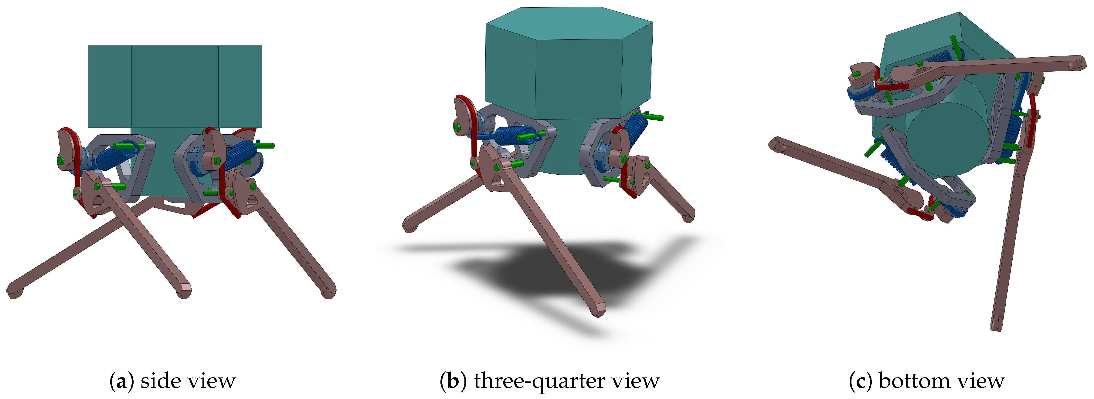
Our approach in achieving a soft landing exploits a mechanism called Variable Radius Drum (VRD) modeled in 2016 by Seriani and Gallina [40] to perform the shaping of the elastic response of a set of linear compression springs in order to provide a constant-force deceleration on the payload. In particular, using the equations from [41], we synthesize a VRD-based mechanism to provide the shaped force to an imaginary 0.9-kg payload within the lander itself in order to mitigate the possible acceleration-induced damage during landing. In

Table 1. Analysis of the state of the art.

Type	References	Touchdown Velocity	Soft-Landing Method	Reusability	Pros	Cons
Real missions	Rosetta [7,8,9]	1.01 m/s	Structural flexibility and electromechanical damping	Yes	Tuning of the damping parameters possible	Not passive, requires control system
	MER A/B [3]	12 m/s	Airbags	No	Light, redundant, passive (after deployment)	Imprecise landing location
	Phoenix lander [49]	2.5 m/s	Powered landing and structural flexibility	Yes	Precise landing location, allows adjustments	Not passive, requires control system, complex system, dust contamination
	MSL [5,50]	0.75 m/s	Sky crane and structural flexibility of the rocker bogies	No	Precise landing location, allows adjustments, limits dust interference	Not passive, requires control system, extremely complex system, high level of autonomy required
Programmed	Omotenashi [31]	20–30 m/s	Airbags	No	Cheap, light, passive (after deployment)	Very imprecise landing location, high impact velocity conditions payload
Hypothetical/ proposed	[30]	2–3.5 m/s	Powered landing and flexible landing legs	Yes	Precise landing location, allows adjustments	Not passive, requires control system, complex system, dust contamination
	[34]	-
	[35]	4 m/s	Powered landing and actuated landing legs	Yes
	[10]	0–3.7 m/s	Crushable structures	No	Cheap, light, reliable, passive, limits dust interference	Must be tuned adequately
	[28]	3 m/s
	[12]	–
	[33]	3.13 m/s	Linear spring with release mechanism	No
Our solution	–	3.13 m/s	VRD-based landing system	Yes	Optimized energy absorption, light, passive, limits dust interference	Complexity of mechanism, rebounds possible

, an overview of the state of the art is illustrated, showing the context in which our proposed solution lies. An illustration of the lander is visible in Figure 1. The elective application is that of landers for space exploration and rovers [24]. The system uses cables and pulleys to transfer the momentum energy to the springs [42,43]. The use of cables can be beneficial to the exploration of space environments because of their lightness and intrinsic modularity [44]. The concept of VRD has seen various applications in the industry for kinematics shaping [41,45], energy efficient springs [43], weight compensation [46], actuation [47,48], and shock absorption [42].

In Section 2, we give some mathematical context to the phenomenon of impact and the soft-landing procedure. In Section 3, we describe the model, both for what concerns the synthesis of the VRD pulley and for the dynamics model that we use to simulate the behaviour during a landing event; furthermore, the model for the springs is illustrated, with emphasis on the VRD-based response; finally, a small space is dedicated to the characterization of the model to be used in the comparison between different landing systems. In Section 4, we present the setup that we use for the dynamic simulations, starting with a VRD reference design obtained through the synthesis (Section 3.1) and loosely optimized; we show how the other landing systems are made to fit the reference behavior in order to allow for homogeneous comparison; finally, we show the numerical results of the simulations of the VRD with focus on the comparative performance between the simulated systems. In Section 5, we discuss the results and provide some insight on the drawbacks and benefits of the proposed technology. Finally, in Section 6, we present our conclusion on the work and we give some foresight in the next steps in this field of research.

2. The Mechanics of Impact and Landing

Landing can be defined as the phase of the mission where the vehicle impacts the ground; the severity of the impact relates to the potential damage which could be caused to the structure and to the payload.

Referring to Figure 2, we can determine the kinetic energy of the object as $E_{kin}=m{\dot{y}}^2/2$. If we consider that the lander starts its fall at a height of $y_0$ (thus, $\dot{y}(y_0)=0$) and ends its motion at a standstill in $y_S$, we can calculate the total theoretical kinetic energy as $E_{kin,th}(y_S)=mg(y_0-y_S)$ from the differential on gravitational potential energy. However, since the spring starts accumulating elastic energy from the moment of impact $y_I$, the kinetic energy $E_{kin}$ at $y_S$ will be zero while the elastic potential energy $E_{el}=E_{kin,th}(y_S)$.

It can be noted at this point that the interval between impact ($y_I$) and standstill ($y_S$), which we call the deceleration phase, is where all kinetic and the remaining gravitational potential energy is transformed into elastic energy in the spring. We can define the corresponding distance $\mathsf{\Delta }{y}_{DP}=y_I-y_S$, which allows us to determine that the elastic energy in a linear spring is as follows:

$$E_{el,lin}=\frac{1}{2}k\mathsf{\Delta }{y}_{DP}^2,$$

(1)

where the constant k is the coefficient of elasticity.

During the deceleration phase, the body undergoes a negative acceleration which brings it from velocity $\dot{y}(y_I)$ to $\dot{y}(y_S)=0$. From the force produced by the spring, we can determine the impact deceleration $\ddot{y}$ which acts on the body itself by considering that $F=m\ddot{y}$. It is indeed clear at this point that the deceleration phase is the most critical part of the collision. The impact deceleration $\ddot{y}$ acts directly on the body and its contents, thus influencing the integrity of the payload. It stands to reason that this should be kept as low as possible in order to protect the payload.

In case of simple springs, since the force is linear with relation to the deformation, the resulting deceleration is not uniform.

In order to model nonlinear behaviors, we introduce a more general way to determine the elastic energy stored in a spring. In Figure 3a, the behavior of a linear spring can be seen in terms of its force-deformation plot. Following from the system illustrated in Figure 2, the produced force is linear with respect to deformation. We can also determine a maximum force level $F_{max}$ (which, for linear springs, coincides with the most compressed condition). We can define the elastic energy as follows:

$$E_{el}=-{\int }_{y_I}^{y_S}F(y)dy,$$

(2)

which coincides to the area below the force–deformation line in the plot. This can be applied to nonlinear springs as well due to the fact that $F(y)$ is defined for each y in a continuum.

It is useful to define an index ${\eta }_E$ to quantify the efficiency of the spring in absorbing energy while remaining below a set $F_{max}$ to protect the payload. In order determine ${\eta }_E$, we need to first determine the theoretical maximum energy which can be absorbed into an ideal spring. By referring to Equation (2), we can see this happens when $F(y)=cost=F_{max}$. Thus,

$$E_{el,t{h}_{max}}=F_{max}(y_I-y_S).$$

(3)

We can now define the energy storing efficiency as follows:

$${\eta }_E=\frac{E_{el}}{E_{el,t{h}_{max}}}.$$

(4)

We can see from Figure 3a that, for a linear spring, ${\eta }_E=0.5$. However, there are other types of springs and spring systems that can be implemented to perform impact energy absorption. One is that of preloaded springs, which is reported in Figure 3b, where ${\eta }_E$ varies between 0.5 and 1, and is ultimately dependent on the value of the preload $F_P$ following the relation ${\eta }_E=(1/2)(F_{max}+F_I)(y_S-y_I)$, where $F_I=F_P$. It is important to say, however, that, in order for ${\eta }_E$ to approach 1, the preload $F_P$ would have to be very close to $F_{max}$, leading to bulky and heavy springs. Indeed, an ideal constant-force spring (such as a preloaded spring with $F_P\approx F_{max}$ and null stiffness) would produce the behavior shown in Figure 3c.

3. Model

In order to allow a quantitative approach for the analysis of the landing system, we propose a synthesis methodology for the mechanism itself and a dynamical model to evaluate the behaviour in the relevant use-cases, i.e., landing and impact mitigation.

Referring to the illustration in Figure 1, and to the diagrams in Figure 4, the mechanical model for the lander is shown along with the main angles and other geometrical entities. The contact force is referred to as $F_c$ and is applied to the “foot” of the leg, located at point T. In particular, the mechanism consists in the following key elements:

• a leg, used to translate the impact motion into rotational motion around point P;
• a Fixed Radius Pulley (FRP₂), attached to the leg, around which a cable (red) is wound;
• a Variable Radius Pulley (VRD), around which the same cable (red) is wound;
• another Fixed Radius Pulley (FRP₁), integral to the VRD and around which a second cable is wound;
• a spring, which connects the frame to the second cable (blue).

In Figure 5 the main phases are shown for the mechanism during its operation on the lander. Specifically, Figure 5a shows the initial position, with the preloaded spring at its rest position and the red cable wound on the VRD; the leg is fully closed. This corresponds to the free-flight phase. The deceleration phase is illustrated in Figure 5b, where the VRD cable (red) is being unwound from the leg pulley (FRP₂) and wound around the VRD. At the same time, the spring cable (blue) is being wound on the spring pulley (FRP₂). Finally, in Figure 5c, the angle $\beta$ reaches $\mathsf{\Delta }\beta$ and the travel of the leg is complete, with the VRD completely unwound, both FRPs wound, and the spring completely stressed.

The span of the leg motion during the deceleration phase, i.e., between the initial and final configurations, is described by $\mathsf{\Delta }\beta$; this can be written as follows,

$$\mathsf{\Delta }\beta =u+\varphi +\arcsin \sin (-\varphi -u)+\frac{y_{DP}}{\parallel \mathbf{T}-\mathbf{P}\parallel )}$$

(5)

where $z_{DP}=y_I-y_S$ is the deceleration distance.

The following four distinct shapes of elastic responses will be modeled:

(A)

linear spring,

(B)

preloaded spring (nonzero stiffness),

(C)

preloaded spring (zero stiffness),

(D)

VRD-based spring system.

These describe the vast majority of landing mechanisms in the current state of the art.

3.1. Synthesis of the Variable Radius Drum

The aim of the VRD is to deliver a constant force $F_c$ during impact. Refer to Figure 4a; during the deceleration phase, the leg rotates by the angle $\beta$, driven by the decelerating downward motion of the lander. Thus, the synthesis condition is as follows:

$$F_c(\beta )=const$$

(6)

We define the angle $\mathsf{\Delta }\beta$ as the angle $\beta$ when the leg is at maximum deflection.

The requirement for the synthesis of the VRD is to model the relation between the motion of the cable g and the angle $\alpha$ of the pulley on which the VRD will be integral. See Figure 4b.

The starting point is to find the relation between the angles $\alpha$ and $\beta$. The principle of virtual works is used to link the work performed by the leg and that performed by the spring pulley (FRP₁), as follows:

$$r_1{F}_1\delta \alpha =\parallel (\mathbf{T}-\mathbf{P})\times {\mathbf{F}}_c\parallel \delta \beta$$

(7)

where $r_1$ is the radius of the spring pulley (FRP₁), $F_1$ is the force acting on the spring cable (blue), and $(T-P)$ represents the lever arm to which force $F_c$ is applied. It should be noted that the force $F_1$ produced by the spring can be written as follows,

$$F_1=F_{max}-k{r}_1\alpha$$

(8)

where k is the stiffness coefficient of the spring and $F_{max}$ is the force exerted at the spring deformation limit. It follows easily that the preload $F_{1,p}$ can be written in the following form:

$$F_{1,p}=F_{max}-k{r}_1\mathsf{\Delta }\alpha$$

(9)

From Equation (5), the moment contained in the right-most part of Equation (7) can be rewritten as follows:

$$\parallel (\mathbf{T}-\mathbf{P})\times {\mathbf{F}}_{\mathbf{c}}\parallel =F_c\parallel \mathbf{T}-\mathbf{P}\parallel \cos (u+\varphi -\mathsf{\Delta }\beta +\beta )$$

(10)

At this point, Equation (7) can be rearranged, yielding,

$$\frac{d\beta }{d\alpha }=\frac{F_1{r}_1}{F_c\parallel \mathbf{T}-\mathbf{P}\parallel \cos (u+\varphi -\mathsf{\Delta }\beta +\beta )}$$

(11)

which is a nonlinear differential equation, in light of the transcendent terms containing $\beta$. Once the relation between the angles $\alpha$ and $\beta$ is understood, it is possible to evaluate $g(\alpha )$, as follows:

$$g(\alpha )=r\beta$$

(12)

taking care to note that $g(0)=0$ and $g(\mathsf{\Delta }\alpha )=r\mathsf{\Delta }\beta$. With Equation (11) as a nonlinear differential equation, a closed form solution of type $\beta =f(\delta )$ is not possible. Therefore, numerical methods will be used. In our case, the angle $\mathsf{\Delta }\beta$ is to be determined based on the admissible span of the leg motion during the deceleration phase, as seen in Equation (5).

Using the Dormand-Prince explicit Runge–Kutta ODE single-step solver, which is implemented in MATLAB, a solution to the II order differential equation (Equation (11)) can be found starting from angle ${\beta }_0=0$ and ${\alpha }_0=0$ as initial conditions. This yields a discrete sequence of n angles ${\beta }_j$, corresponding to a sequence of angles ${\alpha }_j$ defined as follows:

$${\alpha }_j={\alpha }_0+j\delta \alpha$$

(13)

where $\delta \alpha =6.28E-4$ is the discretization step. Note that it is necessary to determine the angle $\mathsf{\Delta }\alpha$ corresponding to $\mathsf{\Delta }\beta$. This can be done via linear interpolation, based on the discrete sequence of angles $[{\alpha }_j,{\beta }_j]$, as follows:

$$\mathsf{\Delta }\alpha ={\alpha }_{\lambda }+(\mathsf{\Delta }\beta -{\beta }_{\lambda })\frac{({\alpha }_{\lambda +1}-{\alpha }_{\lambda })}{({\beta }_{\lambda +1}-{\beta }_{\lambda })}$$

(14)

where $\lambda$ is the index of the last value of $\mathsf{\Delta }\beta$ for which ${\beta }_{\lambda }\le \mathsf{\Delta }\beta$. It follows logically that ${\beta }_{\lambda +1}>\mathsf{\Delta }\beta$.

The framework developed by Seriani et al. [42] can be used to determine the geometry of the VRD pulley. In fact, referring to Figure 4c, the VRD can be described as a continuously differentiable curve defined by points ${\mathbf{p}}_t$ in the reference frame $\langle {\xi }_1,{\zeta }_1\rangle$, as follows:

$${\mathbf{p}}_t=\mathbf{T}(\alpha )\left\{\begin{array}{c}{C}_d\\ 0\end{array}\right\}+\mathbf{T}\left(\alpha \right)\mathbf{T}\left(-\gamma \right)\mathbf{T}\left(-\frac{\pi }{2}\right)\left\{\begin{array}{c}{l}_t\\ 0\end{array}\right\}$$

(15)

where

$$\gamma =\arccos \left(\frac{1}{C_d}\frac{dg}{d\alpha }\right)l_t=\frac{C_d\sin \gamma }{1+\frac{\frac{d^{2}g}{d{\alpha }^2}}{\sqrt{C_d^2-{\left(\frac{dg}{d\alpha }\right)}^2}}}\mathbf{T}(\alpha )=\left[\begin{array}{cc}\cos \alpha & -\sin \alpha \\ \sin \alpha & \cos \alpha \end{array}\right]$$

(16)

Furthermore, from Equation (12), following differentiation with respect to angle $\alpha$, the following is true,

$$\frac{dg}{d\alpha }=r\frac{d\beta }{d\alpha },\frac{d^{2}g}{d{\alpha }^2}=r\frac{d^2\beta }{d{\alpha }^2}$$

(17)

which can be approximated using a finite differences method.

In Figure 6, the result of the synthesis of a VRD is shown in both the start ($\alpha =\mathsf{\Delta }\alpha$) and end positions ($\alpha =0$), i.e., closed ($\beta =\mathsf{\Delta }\beta$) and open leg configuration ($\beta =0$), respectively.

3.2. Dynamical Model

The lander can be modeled as a rigid body system composed of 2 basic elements: the chassis and the legs. Since there is a three-fold radial symmetry with respect to a vertical axis aligned with the center of mass of the lander (see Figure 1), a one-third model can be used for each leg. For the description of the variables used in the following model, refer to Figure 7.

If we consider the chassis of mass m of the lander, the equilibrium of forces and moments yield

$$\left\{\begin{array}{cc}\hfill F_{cst,x}-R_x& =0\\ \hfill mg-m{\ddot{y}}_G-R_y& =0\\ \hfill \parallel {\mathbf{M}}_k\parallel +\parallel {\mathbf{M}}_c\parallel +\parallel {\mathbf{M}}_{cst}\parallel & =0\end{array}\right.$$

(18)

where $F_{cst,x}$ is the x-component of the constraint force acting on the virtual vertical slide, $M_{cst}$ is the moment acting on the same object, and $M_c=-c\dot{\alpha }$.

Regarding the leg, the equilibrium can be written as follows:

$$\left\{\begin{array}{cc}\hfill R_x-m_l{\ddot{x}}_Q+F_x& =0\\ \hfill R_y-m_l{\ddot{y}}_Q+m_{l}g+F_y& =0\\ \hfill {\lambda }_{\overline{\mathbf{GQ}}\times x}{m}_l{\ddot{x}}_Q+\\ \hfill {\lambda }_{\overline{\mathbf{GQ}}\times y}{m}_l{\ddot{y}}_Q+\\ \hfill {\lambda }_{\overline{\mathbf{GQ}}\times x}{m}_{l}g+\\ \hfill \parallel {\mathbf{M}}_k\parallel +\parallel (\mathbf{P}-\mathbf{G})\times \mathbf{F}\parallel & =0\end{array}\right.$$

(19)

where the letter $\lambda$ denotes the following terms:

$$\left\{\begin{array}{cc}\hfill {\lambda }_{\overline{\mathbf{GQ}}\times x}& =(\mathbf{Q}-\mathbf{G})\times \widehat{x}\\ \hfill {\lambda }_{\overline{\mathbf{GQ}}\times y}& =(\mathbf{Q}-\mathbf{G})\times \widehat{y}\\ \hfill {\lambda }_{\overline{\mathbf{PQ}}\times x}& =(\mathbf{Q}-\mathbf{P})\times \widehat{x}\\ \hfill {\lambda }_{\overline{\mathbf{PQ}}\times y}& =(\mathbf{Q}-\mathbf{P})\times \widehat{y}\end{array}\right.$$

(20)

In order to write the system described in Equation (19) in terms of ${\ddot{x}}_G$ and ${\ddot{y}}_G$, coherently with Equation (18), we can write

$$\left\{\begin{array}{c}\hfill x_Q=x_G+\parallel \mathbf{Q}-\mathbf{G}\parallel \cos \phi +\varphi \\ \hfill y_Q=y_G+\parallel \mathbf{Q}-\mathbf{G}\parallel \sin \phi +\varphi \end{array}\right.$$

(21)

The double differentiation of Equation (21) yields the following:

$$\left\{\begin{array}{cc}\hfill {\ddot{x}}_Q& ={\ddot{x}}_G-\parallel \mathbf{Q}-\mathbf{G}\parallel \cos (\phi +\varphi ){\dot{\varphi }}^2-\parallel \mathbf{Q}-\mathbf{G}\parallel \sin (\phi +\varphi )\ddot{\varphi }\\ \hfill {\ddot{y}}_Q& ={\ddot{y}}_G-\parallel \mathbf{Q}-\mathbf{G}\parallel \sin (\phi +\varphi ){\dot{\varphi }}^2+\parallel \mathbf{Q}-\mathbf{G}\parallel \cos (\phi +\varphi )\ddot{\varphi }\end{array}\right.$$

(22)

The force F represents the interaction between the ground and the skid, located at point P. In this setting, a spring-damper system was chosen as the model for the soil, assuming dynamic Coulomb friction at all times [24].

$$\mathbf{F}=[\begin{array}{c}{F}_{gd,\mu }\\ F_{gd,k}+F_{gd,c}\end{array}],$$

(23)

where the terms $F_{gd,\mu }$, $F_{gd,k}$, and $F_{gd,c}$ have the following behaviour,

$$F_{gd,\mu }=\left\{\begin{array}{cc}-{\dot{x}}_P{\mu }_{gd}\hfill & \mathrm{if}∥{\dot{x}}_P∥>v_{\mu ,tol}\\ 0\hfill & \mathrm{if}∥{\dot{x}}_P∥\le v_{\mu ,tol}\end{array}\right.,F_{gd,k}=\left\{\begin{array}{cc}-y_P{k}_{gd}\hfill & \mathrm{if}{y}_P<0\\ 0\hfill & \mathrm{if}{y}_P\ge 0\end{array}\right.,F_{gd,c}=-{\dot{y}}_P{c}_{gd}$$

(24)

The equations described in Equation (18) and Equation (19) can be time-integrated using a direct approach. Care must be taken in the choice of a sufficiently small timestep $dt$ due to the high-frequency components of the vibration given by the high ground rigidity. Typically, the components pertaining to the mechanism and the lander itself have very low natural frequencies [24,42] and are thus well modeled even with a large $dt$.

3.3. Stiffness Model

The behavior of each of the spring systems described in Section 3 can be described effectively by the term $\parallel {\mathbf{M}}_k\parallel$. This term is then plugged in the dynamics simulator presented in Section 3.2.

In particular, for the linear non-preloaded spring (case (A), as seen in Section 3),

$$\parallel {\mathbf{M}}_k\parallel =k_{lin}\varphi$$

(25)

where $k_{lin}$ is the linear stiffness coefficient of the spring. For the preloaded spring (items (B) and (C)) a more complex formulation is necessary to capture the bi-elastic behavior [42]:

$$\parallel {\mathbf{M}}_k\parallel =\frac{2}{\pi }{M}_0\arctan (f\varphi )+k\varphi$$

(26)

where f characterizes the sharpness of the curve and $M_0$ is the preload. Finally, the VRD response (item (D)) can be described using the geometrical considerations expressed in Section 3.1, as follows:

$$\parallel {\mathbf{M}}_k\parallel =\left\{\begin{array}{cc}\hfill k\varphi & \mathrm{if}\varphi <0\\ \hfill \frac{2}{\pi }{M}_0\arctan (f\varphi )+k\varphi & \mathrm{if}\varphi \ge 0\end{array}\right.$$

(27)

In Figure 8a the reader can see the force-angle plots for the springs presented above, taking care of considering that ${\beta }^{\prime }\equiv \varphi$. Note that the system based on the preloaded spring and the VRD system are very similar. However, the latter provides a compensation mechanism for the rotation of the leg of the lander. This effect can be seen in the upward curvature of the red dot-dashed line in the plots.

3.4. Characterization of the Model

The model described in Section 3 is rather complex, and its interpretation and the evaluation of its performance require some additional formal aspects; these will be dealt with in this section. We start by defining the deceleration energy $E_d$, as follows:

$$E_d={\int }_{y_0}^{y_S}{F}_{y}d{y}_G=E_{el}$$

(28)

which follows from Equation (2). Then, we define the maximum body deflection ${\mathsf{\Delta }}_{max}$ for the lander, as follows:

$${\mathsf{\Delta }}_{max}=\underset{t\le t_S}{\max }\left(s\sin \left({\beta }^{\prime }(t)\right)\right)$$

(29)

The quantity $D=y_S-y_0$ or “effective drop” is the distance it takes for the lander barycenter $\mathbf{G}$ to reach a velocity ${\dot{y}}_G=0$ and takes into account both the height above the floor $H=y_I-y_0$ and the yield of the soil (modeled here as a spring-damper system).

The second point we make is that of the deceleration space $Y_d=y_S-y_I$, referring to Figure 2. This is the span of travel along the y-direction where the system converts part of its kinetic energy into elastic potential energy in the spring; the remaining energy dissipates as heat in the dampers or due to friction. This energy transfer is the leading factor in the behavior of the deceleration of the lander during the collision, which is described by ${\ddot{y}}_G$.

4. Numerical Simulations

In order to show the behavior of the VRD landing system and to give some context to the numbers, a comparison between the spring configurations (A)–(D) (see Section 3) is shown in the following. For each, two sub-configurations are shown, with and without damping.

One additional situation is defined here: the theoretical best configuration. This is characterized by a perfectly constant deceleration; referring to the quantities described in Section 3.4, one can write the lowest possible value of deceleration that satisfies the constraints on the deceleration space and kinetic energy to dissipate:

$${\ddot{y}}_{G,th}=E_d/Y_d$$

(30)

4.1. VRD Reference Design

The first step for our comparison is the determination of a design for the VRD suspension system. In this context, we will not delve deep into finding the best possible solution for the mechanism but rather will settle for a “good enough” iteration. This will constitute the reference design to which we will compare configurations (A)–(D).

From the model, described in Section 3, it is apparent that the VRD system has many degrees of freedom for what concerns the design. Among the many possible combinations of parameters, we chose to define our parameterization for the design of the mechanism $\mathrm{\Xi }$, as follows:

$$\mathrm{\Xi }=f\left(r,r_1,m,w,s,Y_d\right)$$

(31)

The means with which we find this configuration of the parameters described in Equation (31) is that of using an optimization technique (more specifically a single-objective genetic algorithm) which responds to the following statement:

$${\mathrm{\Xi }}_{opt}=\underset{r,r_1,m,w,s,Y_d}{\min }\left(\frac{1}{{\eta }_E}\right)$$

(32)

where

$$\begin{array}{c}r\in [\underline{r},\overline{r}],r_1\in [\underline{r_1},\overline{r_1}],m\in [\underline{m},\overline{m}],w\in [\underline{w},\overline{w}],s\in [\underline{s},\overline{s}],Y_d\in [\underline{Y_d},\overline{Y_d}]\end{array}$$

(33)

where the terms $\underline{\ast }$ and $\overline{\ast }$ indicate respectively the lower and upper bounds of the domain of existence of the related parameter ∗.

The results of the optimization stated in Equation (32) are shown in

Table 2. VRD reference design: design parameters values and characteristics.

Parameter (Fixed)	Value	Parameter (Optimized)	Value	Characteristics	Value
$F_{max}$	220 N	r	0.0500 m	$E_d$	1.4715 J
k	14,700 N/m	$r_1$	0.0032 m	$M_0$	2.3022 Nm
$\phi$	$-{20}^{°}$	m	0.9000 kg	$F_y$	11.317 N
g	9.81 m/s${}^2$	w	0.0200 m	${\eta }_E$	44.692%
H	0.500 m	s	0.2527 m	${\eta }_{E,eff}$	99.992%
c	0.010 Ns/m	$Y_d$	0.1300 m	D	0.5744 m
$c_{gd}$	0.400 Nms			${\ddot{y}}_{G,max}$	34.1288 m/s${}^2$
$k_{gd}$	4000 N/m
${\mu }_{gd}$	0.0

.

In the following, this configuration will be used as the baseline for comparison. It will provide the deceleration energy $E_d$, the effective drop D, as well as the other characteristics.

In order to perform a coherent comparison, the quantities ${\epsilon }_{{\ddot{y}}_{G,max}}$ and ${\epsilon }_{\eta ,E,eff}$ will be used as the main performance indicators of the different configurations, as follows:

$$\begin{array}{c}{\epsilon }_{{\ddot{y}}_{G,max}}=\frac{|y_{G,max}-y_{G,max,ref}|}{y_{G,max,ref}}\\ {\epsilon }_{{\eta }_{E,eff,max}}=\frac{|{\eta }_{E,eff,max}-{\eta }_{E,eff,ref}|}{{\eta }_{E,eff,ref}}\end{array}$$

(34)

4.2. Setup

The different spring systems vary widely in terms of their dynamic response. In order for the comparison to be effective, referring to Section 3.4, a few points should be defined. The aim is to determine the correct parameters for configurations (A)–(C) to be energetically equivalent to the VRD reference design (D). The main parameters related to the spring system are the spring stiffness k, the effective drop D, and the preload torque $M_0$.

Since D is very influential to the kinetic energy at impact, its relation to the terrain yield mechanics make it difficult to interpret and define. For this reason, the parameter we chose for the characterization of the drop phase is the dissipation energy defined in Equation (28). From the definition of this value, the drop D can be computed. It follows logically that, in order to have an homogeneous (iso-energetic) comparison of the impact mechanics, the dissipation energies $E_d$ should be the same for all springs.

Note also that the quantity $Y_d$ is specific of the lander design and should be considered a fixed design parameter; for these reasons, in order to allow for homogeneous comparison conditions, we consider this value constant through all configurations.

To summarize, we elect to fix the dissipation energy $E_d$ and the deceleration space $Y_d$ for all configurations. This will provide energetically equivalent models that satisfy the geometrical constraints of the lander.

In order to find viable solutions for all configurations, we use an optimization technique; this is necessary due to the nonexistence of closed-form solutions. The method minimizes the following objective function in terms of two parameters ${\lambda }_1$ and ${\lambda }_2$, which are different depending on the adopted type of spring system:

$$\underset{{\lambda }_1,{\lambda }_2\in \mathbb{R}}{\min }\left(\max \left({\epsilon }_Y({\lambda }_1,{\lambda }_2),{\epsilon }_E({\lambda }_1,{\lambda }_2)\right)\right)$$

(35)

where ${\epsilon }_Y({\lambda }_1,{\lambda }_2)$ and ${\epsilon }_E({\lambda }_1,{\lambda }_2)$ are defined as follows in terms of the nominal quantities $Y_d^{*}$ and $E_d^{*}$, which are defined by the VRD design:

$$\left\{\begin{array}{cc}{\epsilon }_Y& =\left|\frac{Y_d^{*}-Y_d({\lambda }_1,{\lambda }_2))}{Y_d^{*}}\right|\\ {\epsilon }_E& =\left|\frac{E_d^{*}-E_d({\lambda }_1,{\lambda }_2))}{E_d^{*}}\right|\end{array}\right.$$

(36)

Regarding the $\lambda$-parameters,

Table 3. Numerical simulation: $\lambda$-parameters.

Spring Design	${\mathit{\lambda }}_1$	${\mathit{\lambda }}_2$	Other
Linear non-preloaded	$k_p$	D	$M_0=0$
Linear preloaded (zero stiffness)	$M_0$	D	$k_p=0$
Linear preloaded	$k_p$	D	$M_0=1$

summarizes which of the design parameters are attached in the specific configurations. More specifically, each needs to be fitted to the VRD reference design main performance parameters, namely $E_d^{*}$ and $Y_d^{*}$. As discussed in the previous paragraphs, these quantities define precisely the energy and dynamics of the system.

4.3. Results

In this section, the results for the synthesis of the VRD-based mechanism are shown as well as that of the dynamics behaviour in all cases defined at the beginning of Section 4.

As stated in the previous sections, a series of configurations are considered to demonstrate the variability of the dynamical performance of the suspension system. In

Table 4. Numerical simulation results: The percentage values in parentheses for ${\epsilon }_{{\ddot{y}}_{G,max}}$ and ${\epsilon }_{{\eta }_{E,eff,max}}$ are relative to the theoretical best deceleration profile ${\ddot{y}}_{G,th}$; those not in parentheses are relative to the VRD reference design.

Spring Design	Damping	$\mathit{\lambda }$-Parameters		Max. Deceleration		Energy Storage Efficiency
		${\mathit{\lambda }}_{\mathbf{1}}$	${\mathit{\lambda }}_{\mathbf{2}}$	${\ddot{\mathit{y}}}_{\mathit{G},\mathit{max}}$	${\mathit{\epsilon }}_{{\ddot{\mathit{y}}}_{\mathit{G},\mathit{max}}}$	${\mathit{\eta }}_{\mathit{E},\mathit{eff}}$	${\mathit{\epsilon }}_{{\mathit{\eta }}_{\mathit{E},\mathit{eff},\mathit{max}}}$
		[m]		[ms${}^{\mathbf{-}\mathbf{2}}$]	[-]	[-]	[-]
Linear no-preload	Yes	$k_p=6.59$	$D=0.4801$	$59.80$	$+58.63\%$	$55.88\%$	$-20.54\%$
Linear prel. ($k_p=0$)	Yes	$M_0=2.27$	$D=0.4827$	$50.27$	$+33.35\%$	$46.76\%$	$-33.51\%$
Linear preloaded	Yes	$k_p=3.67$	$D=0.4803$	$44.59$	$+18.28\%$	$64.73\%$	$-7.92\%$
VRD system (ref.)	Yes	$M_0=2.47$	$D=0.4808$	$37.70$	$(+28.80\%)$	$70.33\%$	$(-29.67\%)$
Linear no-preload	No	$k_p=6.59$	$D=0.4801$	$130.07$	$+142.77\%$	$29.32\%$	$-52.52\%$
Linear prel. ($k_p=0$)	No	$M_0=2.27$	$D=0.4827$	$67.28$	$+25.56\%$	$44.27\%$	$-28.32\%$
Linear preloaded	No	$k_p=3.64$	$D=0.4803$	$100.40$	$+87.39\%$	$36.53\%$	$-40.85\%$
VRD system (ref.)	No	$k_p=2.47$	$D=0.4808$	$53.58$	$(+83.05\%)$	$61.76\%$	$(-38.24\%)$
VRD ($m_l=0.5m_{l,ref}$)	Yes	$M_0=2.50$	$D=0.4739$	$31.09$	$(+7.29\%)$	$89.73\%$	$(-11.44\%)$
VRD ($m_l=0.2m_{l,ref}$)	Yes	$M_0=2.53$	$D=0.4859$	$29.67$	$(+2.45\%)$	$95.05\%$	$(-5.21\%)$
VRD ($m_l=0.1m_{l,ref}$)	Yes	$M_0=2.53$	$D=0.4895$	$29.31$	$(+1.45\%)$	$96.65\%$	$(-3.46\%)$
Theoretical best	No	—	—	$29.27$	—	$100.0\%$	—

, the results are shown in aggregate form for all 8 configurations, along with the deviation from the reference design (in this case the VRD, both in the case of a damped and non-damped system). In addition, three additional configurations are shown relative to the variation of the mass of the leg $m_l$. Note that each configuration is obtained following the methodology described in Section 4.2, reaching a fit of approximately ${10}^{-8}$ for Equation (36): incidentally, these values are reported in the same table (see $\lambda$-parameters). As such, the parameters $E_d$ and $Y_d$ are equivalent within the set of considered configurations. This allows a comparison between homogeneous systems.

The values for maximum deceleration ${\ddot{y}}_{G,max}$ and for energy storage efficiency ${\eta }_{E,eff}$ show that, depending on the configuration, wide differences can occur within the dynamic behavior. In particular, the maximum deceleration varies as much as by $60\%$ in the case of damped systems. For non-damped systems, it reaches values in excess of $130\%$ compared to the reference design (the VRD system, (D)).

For the sake of completeness, the results for the VRD reference design are compared to the theoretical best deceleration profile, as well (see Equation (30)). This yields rather unsatisfactory results: approximately $30\%$ in the best case (damped (D) system) and $83\%$ in the other (non-damped). However, in the case of a VRD where the mass of the leg $m_l$ is smaller, this result in the damped case decreases to a value of $1.45\%$.

The plots in Figure 9 and Figure 10 show the behavior of the system in the time-domain. More specifically, in Figure 9, the deceleration profile ${\ddot{y}}_G$ is shown for each damped configuration with regards to the coordinate $G_y$ of the barycentre G. The red line shows the moment in time when the deceleration is complete. It can be seen from the bottom plots that the deceleration shows large oscillations between roughly 30 and $50\%$ of the peak value. Non-damped configurations are not shown.

In Figure 10, a comparison is shown between the behavior of the 4 damped configurations and that of the theoretical best deceleration profile ${\ddot{y}}_{G,th}$; furthermore, the evolution of the deceleration energy $E_d$ is plotted against that of the theoretical one.

Finally, in Figure 10, the evolution of the oscillations is shown to change with respect to the mass $m_l$ of the leg of the lander, reflecting the results shown in Table 4. Note that, for each of these simulations, the total mass of the lander, i.e. $m+m_l$ is constant and equal to that of the VRD reference design.

4.4. Parameter Characterization

The behavior of the system is dependent on a multitude of parameters: environmental, structural, and dynamical. In this section, the influence of mass, gravity, and the stiffness and friction coefficients of the ground will be investigated. The selection of these parameters was due to the large implications that these have in the dynamics of the landing system during impact. In Figure 11, the results are reported in graphical form with the discretization and domain described in

Table 5. Parameters characterization: domain and discretization.

Parameter	Min	Max	Increment
m (kg)	0.47	1.88	0.0047
g (ms${}^{-2}$)	0.98	11.77	0.1090
$k_{gd}$ (N/m)	2000.00	8000.00	60.6061
${\mu }_{gd}$ (-)	0.00	0.60	0.0061

. The other parameters are those of the reference design, reported in Table 2.

5. Discussion

From the extensive analysis presented in the previous sections and specifically considering the results illustrated in Section 4.3, a complete analysis and critical review will be presented on the dynamic response of a landing system based on a VRD mechanism. In this section, the focus will be mainly on the damped configurations, leaving the non-damped ones as a secondary reference.

Let us consider the results in Table 4. In particular, we can see that the value of the deceleration ${\ddot{y}}_G$ for the VRD system reaches a maximum value of 37.70 ms${}^{-2}$. This value is rather large compared to the theoretical optimum (28.27 ms${}^{-2}$ but is still the smallest compared to the other solutions. This can be appreciated graphically from Figure 9a, compared to the second best solution (Figure 9d).

An important feature to discuss is that of the rapid oscillations, which are visible throughout the deceleration of the payload, as visible in Figure 12. The first aspect which is important to cover is that of the reduction in time of said oscillation; this is a direct consequence of the damping present in both the model of the ground or soil and that of the joint itself. The second aspect is related to the origin of these oscillations: in fact, the figure shows that the high-frequency vibration of the leg is consistent with this effect and tends to disappear when the parameter $m_l$ (the mass of the leg) is reduced, as visible in the figures Figure 12a–d. The associated values of the deceleration ${\ddot{y}}_G$ indeed decrease by a large margin, reaching 29.31 ms${}^{-2}$ for the case of $m_l=0.1m_{l,ref}$, which has a deviation of 1.45% with respect to the theoretical best value.

In this work, the vibration of the leg is not analyzed in depth. While the effects of damping and of the mass of the leg have a degree of impact in the magnitude of the peaks of deceleration, the effect on the dissipated energy is very low; this statement can be supported by looking at the bottom row of the plots in Figure 10d, where the peaks of the dissipation energy $E_d$ are not significantly lower than those of the theoretical curves $E_{d,th}$. In other words, the very small difference between the peak of the two curves is the portion of energy lost as heat due to the damping effect introduced in the hinge and in the ground.

The last general aspect that may be discussed is that of the direct comparison between the deceleration of the payload ${\ddot{y}}_G$ and the theoretical best deceleration ${\ddot{y}}_{G,th}$. Taking as reference the plots in the top row of Figure 10, it is rather clear that the response of the VRD mechanism follows closely the shape of the theoretical curve. Graphically, this proves that the shaping of the dynamic response of the suspension system with the methodology presented in this paper is effective. The hard numbers from the simulations support this thesis, as already seen from Table 4. Indeed, the energy storing efficiency parameter ${\eta }_{E,eff}$ of the VRD configuration is the best amongst those tested by a large margin, approximately $8\%$.

It is interesting to note one aspect that may be considered to some extent fortuitous; even though the storing efficiency parameter ${\eta }_{E,eff}$ for the linear preloaded ($k_p=0$) configuration (Figure 10c) is the closest to the one of the VRD, if the peak deceleration ${\ddot{y}}_{G,max}$ is considered, configuration d, i.e., configuration linear preloaded ($k_p>0$), is the closest to the VRD. This remarkable result can be explained by carefully analyzing and comparing Figure 10d,c. The large oscillations due to the leg vibrations tend to be low energy and thus are easily dissipated by the dampers in the ground and in the leg hinge; the effect of this is that the magnitude decreases rapidly while approaching the deflection limit (shown by the dash-dotted line), which offsets the first part of the deceleration curve, while having a small effect on the last part, which is higher by itself. On the other hand, in the case of the zero-stiffness case (Figure 10c), the first part of the curve is supposed to be higher and the oscillations tend to worsen the situation.

From the plots presented in Figure 9 and Figure 10, it is apparent that, once the inversion point is reached, the acceleration keeps going and the simulated lander tends to bounce upwards. In a real scenario, this would be undesirable in most situations; however, the scope of this paper is to demonstrate the effects of using a VRD in the first phase of impact with the ground, when the deceleration happens. However, several solutions are possible in order to limit the rebound: for example, the springs could be let loose after the deceleration phase [33]; a possible solution might rely on one-way mechanisms like ratchets to keep the VRD from rotating back into the initial position; finally, the implementation of damping devices either viscous- or friction-based could be considered.

The variation of the parameters related to the dynamics of the system, namely m and g, produce a large variation in behaviour during impact; in particular, as Figure 11a shows, the mass of the lander is inversely proportional to the maximum deceleration ${\ddot{y}}_{G,max}$. This is to be expected since, if the elastic behavior of the VRD remains the same, the energy associated to a less massive lander is lower. Thus, due to the constant force produced by the VRD, the deceleration is expected to be higher. Quantitatively, a variation of the mass from 0.48 kg to 1.90 kg produces a reduction on ${\ddot{y}}_{G,max}$ of approximately 80%.

Conversely, the main effect of the variation of the acceleration of gravity g is that of limiting the feasible solutions, as the same figure shows; no significant change is expected in the maximum deceleration. Indeed, the variation in ${\ddot{y}}_{G,max}$ between the extremes is approximately 9%.

The system is strongly influenced by environmental factors pertaining to the ground. The response surface in Figure 11b shows the influence of the ground stiffness $k_{gd}$ and of the soil friction ${\mu }_{gd}$. We can see that the ground friction is directly proportional to the maximum deceleration ${\ddot{y}}_{G,max}$. This is expected, since friction acts against the motion of the foot of the lander during the rotation of the leg (see Figure 4a), which increases the deceleration force on the lander. Going from a value of ${\mu }_{gd}=0$ to $0.6$ produces a variation of approximately 54% in ${\ddot{y}}_{G,max}$.

On the other hand, the variation of the ground stiffness produces very minor effects on the dynamics of the system. Indeed, a variation of 400% causes a small 20% increase of ${\ddot{y}}_{G,max}$.

6. Conclusions

In this work, a cable-based preloaded nonlinear elastic landing system was presented. The device is based on a preloaded Variable Radius Drum (VRD) mechanism which is able to deliver a very precise torque on the landing legs of the lander. Through mathematical modeling, the VRD geometry was synthesized specifically for this task; the result allowed to perform the shaping of the elastic response of the landing system. This allows to maximize the efficiency in converting the kinetic energy of the fall to potential elastic energy in a spring. The dynamics of the lander equipped with the VRD landing system was modeled, and a simulation engine was implemented. Several other configurations were modeled and simulated in order to offer a comparison for the proposed technology. The results show that the VRD landing system approaches the theoretical limits with a deviation of less than 30%, while the other systems underperform the VRD solution by between 18% and almost 60%. Furthermore, the relation between the oscillation of the leg of the lander is shown with regards to the mass of the leg itself, indicating that the 30% mismatch decreases to close to a value of approximately 1.45%. Finally, a comprehensive analysis on the most influential parameters on the dynamics was illustrated quantitatively; this showed some limitations of the reference VRD design with regards to the gravity value, mass of the lander, and the ground stiffness and friction parameters.

In the future, steps should be taken in the validation of the methodology herein described, especially for what concerns the mechanism elastic response and the dynamics of the lander itself. This validation should take place both numerically with a state-of-the-art dynamic solver and a full 3 d.o.f. model of the lander and, experimentally, taking care to characterize the soil upon impact.

The technology, however, promises to allow reusable landing systems that minimize accelerations to the payload and are at the same time cheap, light, and robust assets that could be important in the design of small U-class cubesat-sized landers.