Abstract
This paper proposes a classification of all non-isomorphic anatomies of an orthogonal metamorphic manipulator according to the topology of workspace considering cusps and nodes. Using symbolic algebra, a general kinematics polynomial equation is formulated, and the closed-form parametric solution of the inverse kinematics is obtained for the coming anatomies. The metamorphic design space was disjointed into eight distinct subspaces with the same number of cusps and nodes plotting the bifurcating and strict surfaces in a cartesian coordinate system . In addition, several non-singular, smooth and continuous trajectories are simulated to show the importance of this classification.
1. Introduction
This paper investigates the cuspidality of the anatomies derived by a metamorphic manipulator structure. Metamorphic manipulators are considered as a new special class of serial open-chain manipulators that have been developed to fulfill the high manufacturing demands (high productivity, low maintenance cost, space-saving, high accuracy etc.) [1].
A metamorphic manipulator consists of rigid links, pseudo-joints and active modules that can be easily and quickly assembled into different arm structures. The metamorphosis is achieved through the pseudo-joints [2], which are used to change the arm anatomy [3]. It was showed that a regular metamorphic manipulator system can be used to achieve high kinematic performance adapted to the tasks’ requirements [4,5].
The first prototypes of modular, reconfigurable robotic arms have been started to come up at the end of the previous century. A modular manipulator system was developed, which consists of actuator modules, rigid links and a control unit and the efficiency of its mechanical hardware and control software [6]. A reconfigurable modular manipulator system (RMMS) with rigid links, intelligent and active joint modules of various sizes was proposed to perform a wide range of simple or more complex tasks thanks to different arm geometries and an embodied sophisticated kinematic, calibration and control software [7]. A rapidly reconfigurable robotic work cell was designed based on component technology with hardware, software and control issues [8] and a fully functional RMMS work cell to perform light machining tasks was introduced [9]. An innovative mechanical conceptual design is proposed for a modular reconfigurable serial manipulator with a unique geometric cubic actuator module design with connecting ports on all faces of the cubic module, so to minimize the total number of passive or active modules [10].
A closed-form kinematics for reconfigurable robots especially with robustness in coping with singularities using Product-of-Exponentials techniques was developed for different arm geometries and DOF’s [11]. The inverse kinematics of a 3R metamorhic manipulators with one pseudo-joint using a feedforward neural network was also presented [12].
A Genetic Algorithm method was used to evaluate the wide range of modular robot assembly geometries, as well as the effectiveness and robustness of the method, was tested using 4-DOF manipulators [13]. Methods for the kinematic synthesis of structure topologies [3], optimal design of a metamorphic manipulator using path dexterity indices for service tasks [14,15] as well as task placement in the presence of obstacles [16] was presented.
Reconfigurable robotic systems were assessed to find the most suitable geometry with high adaptability [17]. An active module with multiple input-output mechanical connection ports was proposed [18] as well as the active joint module has 2 DOF and it can be used as a rotary or pivotal joint. Experimental verification of high kinematic performance of a simple task using metamorphic manipulators was presented [19].
Considering the most representative papers commended above as well as the robotics literature on reconfigurable manipulators it could be concluded that this type of robot attracts the attention of the robotics community and the manufacturing industry. However, apart from the topology and derived anatomies optimality other aspects should be considered to show the advantages of modular reconfigurable manipulators such as the classification of anatomies in cuspidal and non-cuspidal.
A non-redundant robot that can change its arm configuration (posture) without encountering a singularity is defined as cuspidal [20]. The general, necessary and sufficient conditions for a 3R manipulator to be cuspidal was introduced [21].
Serial orthogonal 3R fixed-anatomy manipulators were classified based on the number of cusp points in workspace Groebner Basis and Cylindrical Algebraic Decomposition [22]. The manipulator design parameter space was divided under some hypotheses into domains with a constant number of cusp points. The obtained equations were produced as algebraic polynomials in the D-H parameters. A classification of 3R orthogonal manipulators was presented, taking into account more topological features such as cusps, nodes, accessibility, aspects, voids [23].
Since the metamorphic manipulators have the ability to alter their anatomies there is a need to investigate and classify the anatomies of metamorphic manipulators according to their topological features (cusps, nodes etc.).
The main aim of this paper is to classify all the non-isomorphic kinematic anatomies for an orthogonal 3R metamorphic structure considering topological features such as cusp, node, aspects, generic and non-generic. According to the approach presented in [22,23] a modified analytical work is introduced adaptable to metamorphic structures to classify the cuspidality of their derived anatomies. General and sufficient conditions to investigate these features, as well as the hypersurfaces that separate them, are determined in terms of metamorphic structure parameters. Selected anatomies are used to illustrate the singularities in configuration and their mapping to the workspace.
To highlight the significance of the metamorphic structure workspace topologies in performing non-singular posture changing paths in the operational space, test trajectories are simulated. The joint angles variation, as well as the determinant of the Jacobian matrix for a closed path and a rectilinear trajectory, are used to illustrate the performance of the metamorphic anatomies.
The rest of this article is organized as follows: in Section 2 the proposed method is presented with the illustrative–metamorphic manipulator structure and some preliminary facts about singularities in joint space and workspace, as well as the meaning of non-singular posture changing mode, is given. Subsequently, Section 3 part of the study is devoted to the classification of non-isomorphic orthogonal anatomies based on the metamorphic workspace topology and the complete enumeration is displayed in the metamorphic design space through strict bifurcating surfaces. In addition, sample metamorphic anatomies are selected from each subspace to represent the kinematic behavior of each one in joint space and workspace. In Section 4, the so-called non-singular posture changing phenomenon is simulated with several numerical examples in generic and non-generic arm models. Finally, the article sums up the most significant conclusions.
2. Cuspidality Investigation in Orthogonal—Metamorphic Modular Arm
Cuspidality Investigation in Metamorphic Orthogonal Serial Robotic Arm is the main aim in this paper and the basic concepts are presented in this section. The next subsection presents the Metamorphic Manipulator Structure that was introduced in [2,3,4,5], in order to facilitate the understanding of the proposed method.
2.1. Presentation of Metamorphic Manipulator
The Metamorphic Manipulator belongs to reconfigurable modular robotic systems that could be reconfigured providing a variety of manipulator anatomies adapted to a wide spectrum of task requirements. The mechanism consists of active modules, pseudo-joints, and link modules (rigid links) [3,4,5]. Active modules (Figure 1a) are mechatronic devices, which are fully equipped with an actuator, harmonic drive, failsafe brake, encoder, power electronics, transmissions and sensors. They are designed with a variety of mechanical standardized coupling connector interfaces that can be easily and quickly assembled into different arm structures. In the present study, the active module is considered as a fully rotational joint.
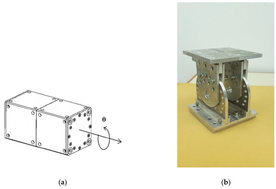
Figure 1.
(a) Active rotational module. (b)Versatile passive joint (pseudo-joint) connector constructed with aluminium and 13 discrete angular positions.
On the other hand, a pseudo-joint constitutes a versatile connector between successive active joints [2], as it is shown in Figure 1b. Pseudo-joints are specially designed to receive discrete values in with a step of 15. Moreover, mechanical interface connectors are developed to align the passive with the active module and couple them together with sufficient strength to transmit the internal forces generated by the load and movement of the arm. The pseudo-joints remain locked in a preselected angular position as the manipulator system is on-line. The angular position of the passive joint is changing offline manually. The transition from an initial robot metamorphic anatomy to a completely different one is feasible with the variation of the pseudo-angles without reassembly of the structure. The pseudo-joint angle alteration changes the D-H parameters of the manipulator structure without changing its kinematic topology.
In this work, three active modules and two pseudo-joints are used to assemble the metamorphic structure and investigate the cuspidality of the derived anatomies, as it is shown in Figure 2a. In Figure 2, is the radius of pseudo-joint, h is the added length of the rotating part of the upper part of the pseudo-joint. The half-width of second and third servo-electric module are and the length of the second actuator is indicated with d. All lengths are measured in meters.
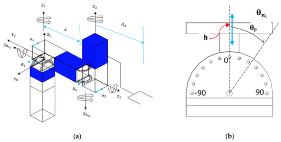
Figure 2.
(a) Orthogonal metamorphic mechanism with local coordinates systems, (b) Side view of passive joint with 13 possible discrete angular positions in .
A specific family of 3R orthogonal metamorphic manipulators with five kinematic parameters and mutually orthogonal active joint axes i.e., is studied. The first passive joint axis is placed perpendicular to the first active joint axis and parallel to the second active module joint axis. In the same way, the second passive joint axis is placed perpendicular to the second actuator axis and parallel with respect to the third active joint axis. Moreover, the actuator limits are ignored, therefore it is considered that . The D-H parameters of the metamorphic manipulator shown in Figure 2 are presented in Table 1 as functions of the metamorphic parameters .

Table 1.
The DH-parameters of the metamorphic manipulator (, , m m m and m).
The kinematic operator projects the joint space to operation space:
where is the cartesian coordinates of the TCP with respect to the global reference frame coinciding with the local coordinate system of the first active joint. Finally, the pseudo-joint angles take 13 discrete values , where .
2.2. The Proposed Method
The metamorphic structure presented in the previous section is used for the introduction of the proposed method. The general, necessary and sufficient conditions for cuspidal 3R serial manipulators are considered to investigate cuspidal anatomies derived from this metamorphic structure. The study focuses on a special family of orthogonal modular manipulators with four distinct kinematic parameters depended on two metamorphic variables while the last joint offset equals to zero . The algebraic parametric polynomial P of fourth-degree in that it solves the inverse kinematics of the depicted mechanism in Figure 2 must have one or more multiple real triple roots [22] or it is equivalent to show that the parametric polynomial system , , has real roots. The above parametric algebraic polynomial system is considered a zero-dimensional system with three equations on three variables where . Thanks to the parametric solution of the polynomial system are obtained the real suitable boundary algebraic polynomials that depend only on D-H parameters shown in Table 1 after removing the imaginary polynomials from the discriminant variety of polynomial system. Thanks to the parametric solution of the polynomial system, the real suitable boundary algebraic polynomials are obtained that depend only on D-H parameters shown in Table 1 after removing the imaginary polynomials from the discriminant variety of the polynomial system. The derived bifurcation equations divide the metamorphic space into subspaces with a constant number of cusp points in workspace.
By the annulment of the determinant of the Jacobian matrix, the singular values could be determined. The investigation of det produces new separating equations [23] that effectively verify the bifurcation equations, which are derived from the solution of the parametric polynomial system. The new separating equations represent intersecting points between singular curves and straight lines in the joint space plane . Moreover, the topological feature of node is taken into account in this investigation. Node is a point in the workspace where the inverse kinematics admits two double solutions [21]. So, the node-based classification is done with pure geometric reasoning by looking at the continuous deformation of workspace [23]. Extra separating equations are produced, which allow us to enumerate both cusp and node points for the depicted kinematic topology in Figure 2. The results are displayed in 3D graphs with strict surfaces which depend only on the metamorphic design parameters . Finally, illustrative metamorphic anatomy is selected from each subspace of metamorphic design parameters 3D space and it is displayed so the singular curves and straight lines in joint space are mapped as the external and internal boundaries of metamorphic workspace.
A considered number of scientific works have been elaborated to plot so the internal as the maximum reach external boundaries in a half cross-section of the total workspace [24,25]. Regional boundaries are singular points in the workspace that the inverse kinematics solutions admit real roots with multiplicity higher than one [26]. However, the most suitable methods investigate the discriminant of the polynomial that provides the inverse kinematics solutions to represent the singular values in half cross-section of the workspace [27]. Furthermore, a variety of important topological features such as cusps, nodes, accessibility and voids are displayed in half cross-section of the metamorphic workspace that assists the engineer to plan discrete or continuous paths in operational space avoiding regional singularities.
Besides, sample metamorphic anatomies are displayed in the same figure in a half cross-section of metamorphic workspace to emphasize the importance of design parameters or the combination of them in the transformation of the workspace (cusp, node, regular, dexterity, manipulability).
Furthermore, non-singular posture changing trajectories with several numerical examples in generic and non-generic models of the metamorphic manipulator are demonstrated. The notion of aspects (singularity free-regions in joint space) helps us to join two inverse kinematic solutions in joint space [28].
3. Classification of Orthogonal Kinematic Non-Isomorphic Configurations of 3R Metamorphic Manipulator according to the Topology of Metamorphic Workspace
Exploiting the homogeneity of mechanism or the geometric analysis of the orthogonal 3R metamorphic manipulator revealed variable DH-kinematic parameters that are dependent on metamorphic design parameters as is shown in Table 1. Assuming continues variation of the pseudo-joints in then the link lengths and the joint offset are continuously varied, while the twist angles remain constant and equal to .
The position of the end effector TCP of the end-effector with respect to the manipulator base is given by:
where, , for . The metamorphic parameters of the manipulator are embodied in the system of Equation (2).
It is known that the inverse kinematics in general 3R manipulators can be solved through a fourth-degree polynomial P in the variable of the last active joint. The Groebner Basis Elimination is used to eliminate the first two active joint variables [22], and to produce a solution that stands for the orthogonal 3R metamorphic manipulator. Following the method presented in [22] the polynomial is derived in the following form:
with , , , , , , , , , , , and , , , . The coefficients of the polynomial P depend on the DH-parameters, including the pseudo-joint variables, and the TCP coordinates .
3.1. Necessary and Sufficient Conditions to Investigate Cuspidality
The necessary and sufficient conditions to recognize a cuspidal 3R manipulator has been introduced in [28]. If and only if there is at least one singular point in its workspace such that the inverse kinematics admits a real triple root, then the manipulator is considered as cuspidal. Therefore, it is equivalent to prove that in Equation (3) admits at least one triple root. Based on the method introduced in [22], a fourth-degree polynomial P has at least one or more triple roots if and only if the polynomial system , admits real radicals. In this way, an algebraic parametric polynomial system S derived to identify and investigate the cuspidal anatomies in orthogonal 3R metamorphic manipulators:
The parametric polynomial system is considered a zero-dimensional system of three equations with three unknowns . Without loss of generality, it is assumed that because a complete rotation around the z-axis of the first active joint lets the system invariant. In addition, and are the constraints for the solution of S. Since is a continuous and differentiable function in , then, and are monotonically increasing function in . The same stands for since A and B are positive quantities. is always positive i.e., in .
The design parameter space must be divided in subspaces such that the sign of the polynomials in Equation (4) is constant. The set of variables should be eliminated to derive polynomials that depend only on DH-parameters.
For this reason, it has been developed general and efficient algorithms to solve parametric algebraic polynomial systems [29,30]. In this way, the parametric polynomial system shown in Equation (4) is solved and the discriminant variety is obtained. After removing the imaginary polynomials, the desired algebraic polynomials are derived that depend only on the following four DH-kinematic parameters . The following system of polynomials indicates the bifurcating equations:
However, only three real polynomials out of five in Equation (5) can be used to the classification according to the number of real roots of Equation (4) i.e., cusp points [31].
Last but not least, it is worth mentioning that Equation (5) has the most general form, as well as the separating equations, are valid for any 3R orthogonal metamorphic manipulator with the selected four kinematic parameters .
In the following sections the investigation of the set of the Equation (5) to classify the metamorphic manipulator according to the number of cusps and the number of nodes.
3.2. Separating Algebraic Equations through Investigation of det
The algebraic set of Equation (5) is used to the classification of open chain 3R orthogonal metamorphic manipulators according to the number of cusp points. The analysis presented in this section is based on the method introduced in [31] without taking into account the assumption that , since in the considered metamorphic structure this parameter depends on the first pseudo-joint angle . The bifurcating surfaces separate the metamorphic design parameters space is subspaces according to the number of cusps as it is shown in Figure 3. The discrete transition of the metamorphic parameters is shown only for the positive angles of the two pseudo-joints . The classification is the same for all possible combinations of pseudo-joints exploiting the symmetry for all the distinct kinematic configurations of the mechanism i.e., (169 kinematic postures). Using Figure 3 the anatomy is derived by selecting the metamorphic parameters based on the number of cusp points.
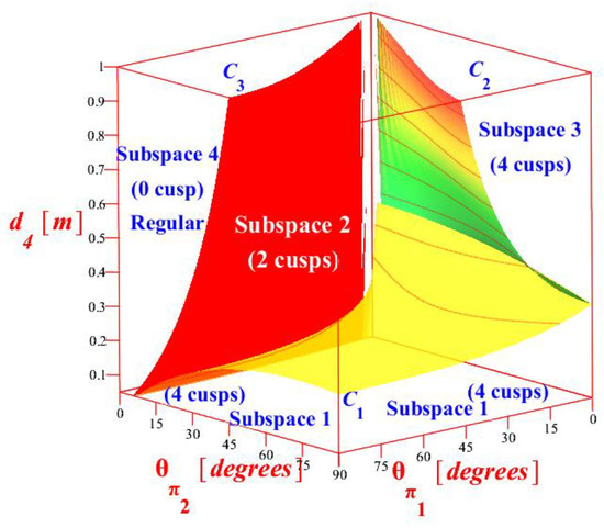
Figure 3.
Surfaces in 3D design metamorphic parameter space and 4 distinct subspaces with the same number of cusp points.
The bifurcating equation in Equation (5) is a biquadratic polynomial in providing the following two roots:
Equations (6) and (7) apply to manipulators with a singular point in the workspace where two cusp points coincide with a node such that Equation (4) has a quadruple root [32]. Equation (6) defines the transition between binary and quaternary manipulators. The surfaces and does not appear in Figure 3 since they are valid for negative values of the metamorphic parameters .
The rest bifurcating equations are derived from the investigation of the determinant of Jacobian det:
Since for the last joint offset, it is assumed that , Equation (8) could be written as two product factors providing the following equations:
Taking into account that , where for and substituting in Equation (9) the following equation is obtained:
Assuming that with then, .
As it shown in Figure 4a the transition from subspace 1 to subspace 2 is characterized by a manipulator for which the singular branch (line) defined by in the joint space is tangent to the singular curve . So, the bifurcating surface separates the metamorphic anatomies with four and two cusps such that,
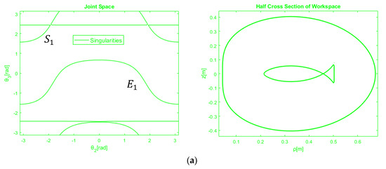
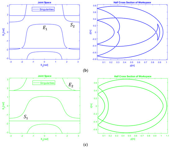
Figure 4.
Selective arm anatomies of the metamorphic structure and singularities are displayed in joint space and half cross section of workspace with the metamorphic parameters: (a) (b) (c)
Since and depend on and respectively then the bifurcating surface , separates the subspace 1 from subspace 2 with four and two cups respectively, as it is shown in Figure 3. Assuming that with , then or .
As it shown in Figure 4b the transition from subspace 2 with two cusps to subspace 3 with four cusps is characterized by a metamorphic anatomy for which the singular branch (line) defined by in joint space is tangent to the singular curve . So, the bifurcating surface separates the manipulators with two and four cusps such that,
The final bifurcating surface is with or .
As it shown in Figure 4c the transition from subspace 2 to subspace 4 is characterized by a manipulator for which the singular branch (line) defined by in joint space is tangent to the singular curve . So, the bifurcating surface separates the manipulators with two and no cusp points (regular workspace topology) given by,
The above surfaces can be verified through Equation (5). The separating equation in Equation (5) is a second-degree polynomial in such that:
Similarly, the bifurcating algebraic equation can be simplified as:
3.3. Classification According to the Number of Nodes
Another important topological feature is the node which is a singular point in the workspace where two singular curves (internal or external) intersect and the polynomial P admits two double roots. In the present section, the distinct kinematic anatomies are classified according to the number of nodes in order to show the deformation of the workspace and hence the non-isomorphism of the kinematic topology.
The method to classify 3R orthogonal fixed manipulators according to the number of nodes is introduced in [23], where analytical algebraic expressions of the surfaces in the parameter space were derived. Analytical algebraic expressions of the surfaces of the parameter space were produced in [23] and are used in this paper to classify the anatomies derived from the considered orthogonal metamorphic structure. The bifurcating surfaces subdivide the metamorphic design space into eight distinct non-isomorphic subspaces with a constant number of cusps and nodes shown in Figure 5. The number of cusp and node points are indicated in parentheses of separating subspaces, respectively. The production of these subspaces is based on the following analysis.
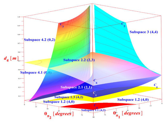
Figure 5.
Separating surfaces in 3D design metamorphic parameter space and 8 distinct subspaces with the same number of cusps and nodes. In every subspace, the first and the second number in the parenthesis indicates the number of cusps and nodes respectively.
Subspace 1 in Figure 3 represents metamorphic anatomies with four cusp points and is divided into three distinct subspaces with different numbers of nodes. The transition between subspace 1.1 to subspace 1.2 is given by the following boundary surface:
Figure 6a shows the singularity curves of a representative metamorphic anatomy from subspace 1.1 that includes generic anatomies with four cusps, two nodes, a void, two subregions with four and one with two inverse kinematic solutions (IKS), respectively shown in Figure 5. Subspace 1.2 in Figure 6b includes metamorphic anatomies with 4 cusps, no nodes, one subregion with four IKS and another one with two IKS, respectively shown in Figure 5. The surface that divides the subspace 1.2 and subspace 1.3 is the following:
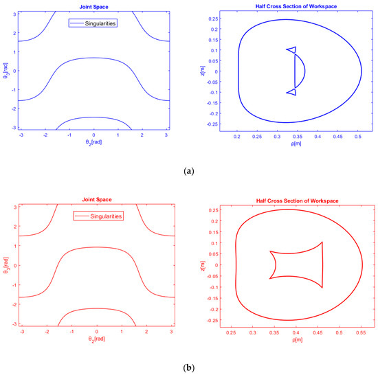
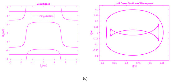
Figure 6.
Selective arm anatomies of the metamorphic structure and singularities are displayed in joint space and half cross-section of workspace with the metamorphic parameters: (a) (b) (c)
Subspace 1.3 in Figure 6c contains metamorphic anatomies with four cusps, two nodes, one region with two and three regions with four IKS respectively and five c-sheets shown in Figure 5. Moreover, subspace 2 in Figure 3 includes metamorphic anatomies with two cusps and it can be subdivided into two neighboring subspaces. The bifurcating surface is formulated as follows,
The transition between subspace 1.3 to subspace 2.1 is expressed by Equation (12) in Figure 4a subspace 2.1 exhibits non-generic metamorphic anatomies with two cusps, one node, two subregions with four and one subregion with 2 IKS respectively and 5 aspects. On the other hand, the transition from subspace 2.1 to subspace 2.2 is defined through the boundary strict surface in Equation (17). In Figure 7a subspace 2.2 includes metamorphic anatomies with two cusps, three nodes, five c-sheets, two subregions with four and two IKS, too as well as the internal intersect with the external boundaries.
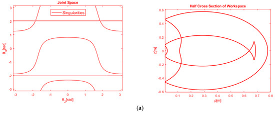
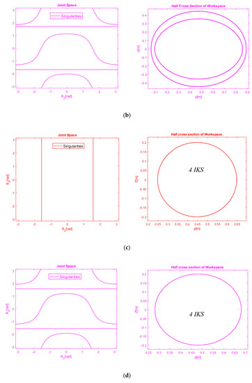
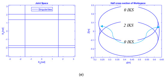
Figure 7.
Selective arm anatomies of the metamorphic structure and singularities are displayed in joint space and half cross-section of workspace with design parameters: (a) (b) (c) (d) (e)
Furthermore, subspace 3 in Figure 4b is a region with four cusps, four nodes, six c-sheets, three subregions with four and two subregions with two IKS, respectively shown in Figure 5.
Finally, the regular subspace 4 in Figure 3 is classified into two spaces through the surface in Equation (17). Subspace 4.1 in Figure 7b includes regular metamorphic anatomies with no nodes, 4 c-sheets, one region with four and two IKS, respectively. Finally, the subspace 4.2 in Figure 4c includes regular non-generic metamorphic anatomies with two nodes, two subregions with 2 and one subregion with four IKS, respectively and four aspects shown in Figure 5.
Moreover, three more arm anatomies are exhibited with at least one zero DH-parameter in Figure 7c,d from subspaces 1.3, 4.1 and 1.3, respectively. The anatomy appeared in Figure 7c is regular with one region of 4 IKS and 2 aspects. Similarly, the manipulator anatomy in Figure 7d has one region of 4 IKS but 4 aspects.
Figure 8a illustrates the transformation of metamorphic workspace with a variation of and m and the corresponding topologies are discerned with different colors. However, the number of cusp points remains constant and equal to four. Moreover, the internal singular segments tend to deform in both axes as well as the location of cusp points is changed too. Moreover, the ratios between the internal subregion i.e., 4 IKS and external one i.e., 2 IKS is changed too.
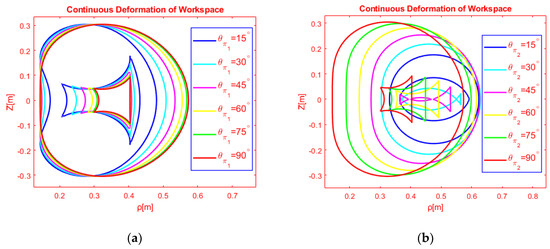
Figure 8.
Continuous direct and inverse projections-mappings of internal and external singularities in a section of metamorphic workspace with the variation only of on left (a) and of on (b) right.
The two DH-parameters depend on the variation of the second passive joint angle as it is shown in Table 1. The variation of in . causes increasing variation for , decreasing and increasing for in , respectively. Consequently, the continuous change of the second pseudo-joint with m changes in a continuous manner the topology of the workspace as it is plotted in Figure 8b. The ratios of internal and external regions are varied, the number of cusp and node points is changing as well as the maximum reach of the end-effector of the mechanism is increasing. Moreover, it is also feasible to switch from generic to non-generic manipulators. Finally, the perpendicular distance from the first joint axes is decreased and as a result, the total workspace is placed closer to the local coordinate system of the base (see Figure 8b in horizontal axis ). Besides, the topological transition from cuspidal to regular anatomy is feasible only with the activation of angular rotation steps of .
In conclusion, it is worth mentioning that the metamorphosis provides various anatomies from a single structure. Kinematic singularities in the workspace of cuspidal manipulators especially the internal boundaries cause serious drawbacks in planning smooth and continuous trajectories and control. However, metamorphic manipulators overcome this fact since it provides a wide spectrum of arm anatomies and hence a variety of regular or cuspidal topological workspaces with varied shape or volume are created. Therefore, engineers can easily select the anatomy required by the given task, based on the classification and analysis introduced in this work. Then, the position of the trajectory or the points for moving objects based on [14,16] can be optimized. In the next section examples of these trajectories are presented.
4. Planning Non-Singular Posture Changing Trajectories
In this section, three distinct metamorphic anatomies that perform non-singular, continuous and smooth trajectories are presented. The active joint angles are illustrated as a function of the distinct steps and the determinant of Jacobian matrix is also plotted to verify the continuity and smoothness of the executed trajectories. In manufacturing and particularly in precision engineering it is important to achieve smooth and very precise trajectories so the manufacturing engineer could select the proper metamorphic anatomy to design the location of such a task avoiding the activation of manipulator breaks close to singularity points. On the other hand, for a different task like point to point motion, the engineer could select a proper metamorphic anatomy using the analysis and the results presented in the previous section.
4.1. Generic Mechanism
The design of a representative anatomy with four cusps and no nodes is based on Figure 3 and Figure 5. So, a metamorphic anatomy is chosen from subspace 2 to perform non-singular mode changing trajectory. The selected anatomy has the metamorphic parameters m. The desired geometric motion is a circle with its center and radius, respectively K and m respectively. The circular path belongs in the vertical plane passing through the Z-axis of the first joint in order to show the singularity free motion. The following function is used to define the path and the trajectory is divided into 100 distinct steps:
where for left-hand or right-hand direction and .
An inner point in 4 IKS region is considered as the starting point of the circle such that and the IKP is solved. Then the respective set of the inverse kinematic solutions are shown in Table 2.
Table 2.
Four inverse kinematic solutions on the starting-ending point of trajectory.
Left-hand rotation is selected i.e., and the TCP of the manipulator performs the circular motion in the half-cross section of the metamorphic workspace (see Figure 9b), as well as the path free of singularity, is traced in the joint space joining the third inverse kinematic solution to the first one in a continuous manner. Besides, the allocation of inverse geometric solutions sets in couples for each aspect is shown in Figure 9a. The joint path is smooth and does not cross any singular curve in aspect .
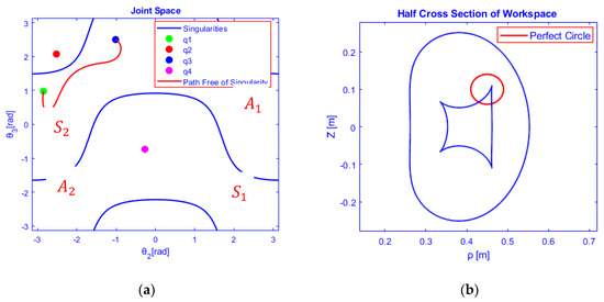
Figure 9.
(a) A free of kinematic singularity path joins two inverse kinematic solutions in aspect , (b) perfect cyclic motion of the TCP encircling a cusp point in the workspace of the selected metamorphic anatomy.
Furthermore, the joints angles are plotted in Figure 10 as a function of discrete steps for the circular path generation. The non-singular posture changing trajectory is feasible without encountering a singularity (outstretched or folded arm) and that can be useful for tasks where collision avoidance is needed.
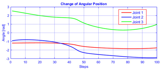
Figure 10.
Joints behavior performing non-singular posture changing trajectory.
Finally, the determinant of the Jacobian matrix is plotted in Figure 11 as a function of the executed steps for a complete circle. The function of determinant is smooth and does not change sign or becomes zero. Moreover, the determinant’s morphology at the beginning of the path is different from the end of the closed path showing the change of posture. Consequently, determinant’s behavior verifies the singularity avoidance during the transition from an inverse kinematic solution to another one.
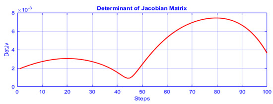
Figure 11.
The determinant of the Jacobian matrix as a function of discrete steps for a perfect circle.
4.2. Non-Generic Anatomy
Non-Generic 3R arm anatomies are considered the open-chain manipulator mechanisms that show two extra critical branches (straight lines) in configuration space . In this section, two different trajectories are planned in two separate non-generic metamorphic anatomies.
4.2.1. Planning Closed Smooth and Continuous Path
A non-generic anatomy is chosen from 3D graphs subspace 2.1 in Figure 5 with two cusps and one node and its singularities are shown in Figure 1. subsequently, the locations of cusp and node points are taken into account to plan a closed path free of singularities. Besides, the appearance of cusp points in half cross-section of the metamorphic anatomy workspace helps the engineer to locate the task to be performed with non-singular posture changing.
The parameters used are: . A circular path is chosen to be performed in metamorphic half cross-section of the workspace . According to the location of cusp and node point in the workspace topology, the center and the radius of the circle are defined to be as follows and m. Then, an inner point in the region with the maximum accessibility is selected as the initial point of the path such that and the inverse kinematics is solved for this point.
The inverse kinematic solutions of Table 3 are distributed in various aspects in configuration space. Only one couple of solutions seems to exist in a single aspect, namely in aspect , while the rest of the IK solutions are placed in different c-sheets and hence a joint path could be executed joining two inverse geometric radical generators.
Table 3.
Four inverse kinematic solutions on the starting-ending point of trajectory.
The motion of the mechanism’s end-effector is described by the desired geometry such that: and , where for left-hand or right-hand direction, .
Right-hand rotation is selected () to perform the trajectory in the chosen aspect . So, taking advantage of the notion of aspects, circles are performed in the characteristic topology of metamorphic anatomy workspace as well as the corresponding joint path is illustrated in the joint space as it is shown in Figure 12. Moreover, it is possible to perform non-singular trajectories even if the end-effector cross internal boundaries in a radial section of the metamorphic anatomy workspace.
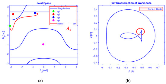
Figure 12.
(a) A continuous and smooth path for two inverse kinematic solutions without change of posture, (b) Circle is performed in half cross-section of metamorphic workspace encircling a cusp point.
The corresponding variation of active joints is plotted as a function of the discrete steps for a complete circular motion. The variation is smooth and the manipulator begins with one posture and ends in a different one, as it is shown in Figure 13.
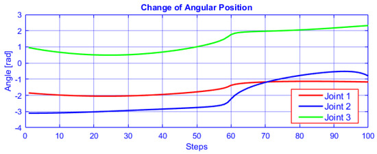
Figure 13.
Change of angular position when the metamorphic anatomy performs a non-singular posture changing trajectory.
It is worth also mentioning that this allocation of solutions in joint space seems not to be actually shown in generic manipulators as we see in Section 4.2.
Finally, the determinant of the geometric Jacobian matrix is displayed in Figure 14. The determinant’s behavior is continuous and smooth. It presents a global minimum in 59th step of trajectory, where the metamorphic anatomy switch inverse kinematic solution in this transition point. The metamorphic manipulator changes inverse solution during the pre-programming trajectory and ends the path with a different posture. This is very important for high precision tasks such as arc welding, cutting or painting in complicated products.
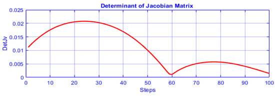
Figure 14.
The behavior of determinant of Jacobian for non-generic metamorphic anatomy.
4.2.2. Rectilinear Trajectory
The 3R orthogonal arm can perform any arbitrary path in a radial section of a metamorphic anatomy workspace. So, a rectilinear trajectory is performed which is important for a wide range of industrial applications such as assembling, grinding, welding, object placement.
Anatomy is selected using the 3D graphs in Figure 15 and the kinematic singularities are displayed in joint space and workspace (see Figure 15), respectively. The anatomy belongs to subspace 3 with the respective design parameters . The topological knowledge of workspace helps the engineer to plan a linear, continuous and smooth path in metamorphic workspace. For this reason, the region with 2 IKS is selected to perform straight lines (two IKS).
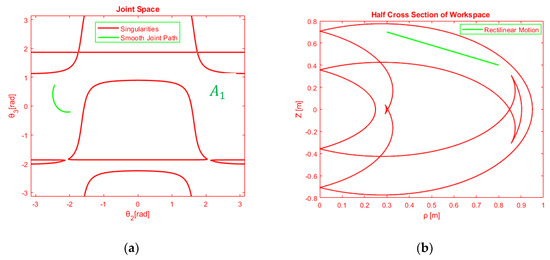
Figure 15.
(a) Smooth curved joint path in aspect and the respective kinematic singularities (b) Rectilinear motion of metamorphic mechanism in half cross-section of the workspace in the region with 2 IKS.
The geometry of the path is defined using linear interpolation and the end-effector is driven with the following geometric motion such that .
The trajectory is divided into 100 steps and takes values in . Continuing the study of rectilinear motion, the joint variation is plotted in Figure 16. The active joints have almost linear behavior during the task execution.
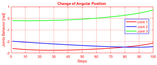
Figure 16.
Active Joints behavior during the rectilinear motion of end-effector.
Finally, the determinant of the geometric Jacobian is plotted in Figure 17 to show the continuous non-singular configuration alteration of the selected anatomy as the end-effector performs the selected rectilinear path in the operational space. In the first 60 steps, the determinant behaves as an increasing function and then decreases until the end of the task.
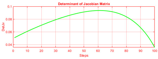
Figure 17.
The continuous function of the determinant of geometric Jacobian for rectilinear trajectory.
5. Conclusions
In this paper, the cuspidality investigation of a metamorphic manipulator is introduced. It embodies the fundamental principles of metamorphosis and the corresponding method allows the engineers to select anatomies from a predefined structure according to topological features such as cusps and nodes.
However, the classification of all non-isomorphic regular or cuspidal metamorphic anatomies revealed novel research results with respect to the metamorphic workspace topological features (cusp, node, shape, volume, accessibility, kinematic dexterity, regular).
This paper revealed also interesting results with respect to kinematic positioning singularities in 3R orthogonal metamorphic manipulators that can be rapidly reconfigured to execute the desired tasks.
The current study shows that the mechanism can be rapidly reconfigured in its arm geometry in order to perform smooth and continuous arbitrary trajectories. The engineers are able to select any non-isomorphic arm geometry from the divided design parameter space thanks to the closed-form solution for the determination of the bifurcating surfaces, that presented in this paper. In this way, regular anatomies are always available for simple tasks as well as cuspidal anatomies could be chosen especially for closed paths i.e., non-singular posture changing trajectory.
The proposed approach enhances the flexibility, extensibility, adaptability and versatility that manufacturing demands can be easily met for a huge variety of reliable and quality products beyond the limitations of well-known, regular fixed-anatomy robots that be able to achieve high task’s performance only for which they were designed.
As for future work, after the selection of the desired subspace based on the topological features, the position of the task can be further optimized based on the methods presented in [14,16] for obstacle avoidance as well as for increasing the kinematic dexterity of the metamorphic manipulator.
Author Contributions
Conceptualization, V.M. and N.A.; methodology, C.K.-P. and V.M.; software, C.K.-P.; validation, C.K.-P., V.M. and N.A.; formal analysis, C.K.-P.; investigation, C.K.-P.; writing—original draft preparation, C.K.-P.; writing—review and editing, V.M. and N.A.; visualization, C.K.-P.; supervision, N.A. All authors have read and agreed to the published version of the manuscript.
Funding
Part of this research conducted by Vassilis Moulianitis has been financially supported by General Secretariat for Research and Technology (GSRT) and the Hellenic Foundation for Research and Innovation (HFRI) (Code: 1184).
Conflicts of Interest
The authors declare no conflict of interest.
References
- Aspragathos, N. Reconfigurable robots towards the manufacturing of the future. In Intelligent Production Machines and Systems-First I* PROMS Virtual Conference: Proceedings and CD-ROM Set; Elsevier: Amsterdam, the Netherlands, 2005; p. 447. [Google Scholar]
- Valsamos, H.; Aspragathos, N. Design of a Versatile Passive Connector for Reconfigurable Robotic Manipulators with Articulated Anatomies and their Kinematic Analysis. In Proceedings of the I* PROMS 2007 Virtual Conference, 2–13 July 2007; Available online: https://app.knovel.com/web/toc.v/cid:kpIPMSTIP1/viewerType:toc/ (accessed on 27 March 2020).
- Valsamos, C.; Moulianitis, V.; Aspragathos, N. Kinematic synthesis of structures for metamorphic serial manipulators. J. Mech. Robot. 2014, 6. [Google Scholar] [CrossRef]
- Valsamos, H.; Aspragathos, N. Determination of anatomy and configuration of a reconfigurable manipulator for the optimal manipulability. In Proceedings of the 2009 ASME/IFToMM International Conference on Reconfigurable Mechanisms and Robots, London, UK, 22–24 June 2009; pp. 505–511. [Google Scholar]
- Valsamos, C.; Moulianitis, V.; Aspragathos, N. Index based optimal anatomy of a metamorphic manipulator for a given task. Robot. Comput. Integr. Manuf. 2012, 28, 517–529. [Google Scholar] [CrossRef]
- Matsumaru, T.; Matsuhira, N. Design and Control of the Modular Manipulator System: TOMMS. J. Robot. Soc. Jpn. 1996, 14, 428–435. [Google Scholar] [CrossRef]
- Paredis, C.J.; Brown, H.B.; Khosla, P.K. A rapidly deployable manipulator system. Robot. Auton. Syst. 1997, 21, 289–304. [Google Scholar] [CrossRef]
- Chen, I.M.; Chen, P.; Yang, G.; Chen, W.; Kang, I.G.; Yeo, S.H.; Chen, G. Architecture for rapidly reconfigurable robot workcell. In Proceedings of the 5th International Conference of Control, Automation, Robotics and Vision, Singapore, 9–11 December 1998; pp. 100–104. [Google Scholar]
- Chen, I.M. Rapid response manufacturing through a rapidly reconfigurable robotic workcell. Robot. Comput. Integr. Manuf. 2001, 17, 199–213. [Google Scholar] [CrossRef]
- Yang, G.; Chen, I.M. Task-based optimization of modular robot configurations: Minimized degree-of-freedom approach. Mech. Mach. Theory 2000, 35, 517–540. [Google Scholar] [CrossRef]
- Chen, I.M.; Gao, Y. Closed-form inverse kinematics solver for reconfigurable robots. In Proceedings of the 2001 ICRA. IEEE International Conference on Robotics and Automation, Seoul, Korea, 21–26 May 2001; Volume 3, pp. 2395–2400. [Google Scholar]
- Tzivaridis, M.; Moulianitis, V.C.; Aspragathos, N.A. Approximation of Inverse Kinematic Solution of a Metamorphic 3R Manipulator with Multilayer Perceptron. In International Conference on Robotics in Alpe-Adria Danube Region; Springer: Berlin, Germany, 2019; pp. 43–50. [Google Scholar]
- Chen, I.M. On optimal configuration of modular reconfigurable robots. In Proceedings of the 4th International Conference on Control, Automation, Robotics, and Vision, Raffles City, Singapore, 4–6 December 1996. [Google Scholar]
- Moulianitis, V.C.; Synodinos, A.I.; Valsamos, C.D.; Aspragathos, N.A. Task-based optimal design of metamorphic service manipulators. J. Mech. Robot. 2016, 8. [Google Scholar] [CrossRef]
- Valsamos, C.; Moulianitis, V.; Synodinos, A.; Aspragathos, N. Introduction of the high performance area measure for the evaluation of metamorphic manipulator anatomies. Mech. Mach. Theory 2015, 86, 88–107. [Google Scholar] [CrossRef]
- Moulianitis, V.; Xidias, E.; Azariadis, P. Optimal Task Placement in a Metamorphic Manipulator Workspace in the Presence of Obstacles. International Conference on Robotics in Alpe-Adria Danube Region; Springer: Berlin, Germany, 2018; pp. 359–367. [Google Scholar]
- Bi, Z.; Gruver, W.A.; Zhang, W.J. Adaptability of reconfigurable robotic systems. In Proceedings of the 2003 IEEE International Conference on Robotics and Automation, Taipei, Taiwai, 14–19 September 2003; Volume 2, pp. 2317–2322. [Google Scholar]
- Li, Z. Development and Control of a Modular and Reconfigurable Robot with Harmonic Drive Transmission System. Master’s Thesis, University of Waterloo, Waterloo, ON, Canada, 2007. [Google Scholar]
- Katrantzis, E.F.; Aspragathos, N.A.; Valsamos, C.D.; Moulianitis, V.C. Anatomy optimization and experimental verification of a metamorphic manipulator. In Proceedings of the 2018 IEE International Conference on Reconfigurable Mechanisms and Robots (ReMAR), Delft, The Netherlands, 20–22 June 2018; pp. 1–7. [Google Scholar]
- Wenger, P. Uniqueness domains and regions of feasible paths for cuspidal manipulators. IEEE Trans. Robot. 2004, 20, 745–750. [Google Scholar] [CrossRef]
- Wenger, P. Cuspidal robots. In Singular Configurations of Mechanisms and Manipulators; Springer: Berlin, Germany, 2019; pp. 67–99. [Google Scholar]
- Corvez, S.; Rouillier, F. Using computer algebra tools to classify serial manipulators. In International Workshop on Automated Deduction in Geometry; Springer: Berlin, Germany, 2002; pp. 31–43. [Google Scholar]
- Baili, M. Analyse et Classification de Manipulateurs 3R à Axes Orthogonaux. Ph.D. Thesis, Ecole Centrale de Nantes (ECN), Université de Nantes, Nantes, France, 2004. [Google Scholar]
- Smith, D.R. Design of Solvable 6R Manipulators. Ph.D. Thesis, Georgia Institute of Technology, Atlanta, GA, USA, 1990. [Google Scholar]
- Tsai, K.Y. Admissible Motions in Manipulator’s Workspace. Ph.D. Thesis, University of Wisconsin-Milwaukee, Milwaukee, WI, USA, 1990. [Google Scholar]
- Kohli, D.; Hsu, M.S. The Jacobian analysis of workspaces of mechanical manipulators. Mech. Mach. Theory 1987, 22, 265–275. [Google Scholar] [CrossRef]
- Ottaviano, E.; Husty, M.; Ceccarelli, M. A Cartesian representation for the boundary workspace of 3R manipulators. In On Advances in Robot Kinematics; Springer: Berlin, Germany, 2004; pp. 247–254. [Google Scholar]
- El Omri, J.; Wenger, P. How to recognize simply a non-singular posture changing 3-DOF manipulator. In Proceedings of the 7th International Conference on Advanced Robotics, Tokyo, Japan, 20–22 September 1995; pp. 215–222. [Google Scholar]
- Lazard, D.; Rouillier, F. Solving parametric polynomial systems. J. Symb. Comput. 2007, 42, 636–667. [Google Scholar] [CrossRef]
- Gerhard, J.; Jeffrey, D.; Moroz, G. A package for solving parametric polynomial systems. ACM Commun. Comput. Algebra 2010, 43, 61–72. [Google Scholar] [CrossRef]
- Baili, M.; Wenger, P.; Chablat, D. A classification of 3R orthogonal manipulators by the topology of their workspace. In Proceedings of the IEEE International Conference on Robotics and Automation, New Orleans, LA, USA, 26 April–1 May 2004; Volume 2, pp. 1933–1938. [Google Scholar]
- Wenger, P.; Chablat, D.; Baili, M. A dh-parameter based condition for 3r orthogonal manipulators to have four distinct inverse kinematic solutions. J. Mech. Des. 2005, 127, 150–155. [Google Scholar] [CrossRef]


© 2020 by the authors. Licensee MDPI, Basel, Switzerland. This article is an open access article distributed under the terms and conditions of the Creative Commons Attribution (CC BY) license (http://creativecommons.org/licenses/by/4.0/).