1. Introduction
With the rapid progress of recent artificial intelligence (AI) and robotic technologies [
1], widely various intelligent robots [
2] have been developed for industrial utilization at factories and warehouses. They have also been developed for collaborative utilization in human societies and facilities in terms of homes [
3], offices [
4], kindergartens [
5], nursing-care facilities [
6], and hospitals [
7]. To perform autonomous locomotion, robots must have capabilities to perform accurate actions and functions of self-localization, path planning and tracking, object recognition, and environmental understanding [
8]. Particularly for mutual dependence and coexistence in human society, robots must have functions to detect people and to recognize human actions and activities effectively [
9].
Simultaneous localization and mapping (SLAM) technologies [
10] have been studied widely as a fundamental approach for autonomous locomotion of mobile robots including drones [
11]. For sequential processing and construction and update of a map for self-location estimation, the computational cost for SLAM increases because probability calculations are necessary for extraction of various map-creation features and for updating real-time positional information. Moreover, the storage capacity for creating environmental maps is expanded exponentially because of the increased observation areas according to enhanced robot locomotion. As an alternative approach, autonomous locomotion using landmarks has been specifically examined as a topic of computer and robot vision (RV) studies [
12]. Advance creation of maps is unnecessary for landmark-based autonomous locomotion and navigation [
13]. Therefore, this approach is effective for considerable reduction of storage capacity and computational costs. However, a difficulty arises: how to set up landmarks. Installing landmarks in advance is another difficulty inherent in this approach.
Landmarks with high discrimination accuracy installed in an environment beforehand according to the purpose and resolution can minimize the ability and performance of a robot in terms of their recognition capability. However, this approach not only involves a pre-installation burden and periodic maintenance, it also involves restrictions for locomotion only in a pre-installed environment. As an approach that requires no landmark pre-installation, visual landmarks (VLs) have been attracting attention in the past two decades [
14]. Herein, VLs are defined as visually prominent objects including text and feature patterns in a scene [
15]. Mohareri et al. [
16] proposed a navigation method using augmented reality (AR) markers as landmarks. Although AR markers have high discriminative performance, their installation involves a great burden and various difficulties. Unlike AR markers, we consider that VLs extracted from general objects have high affinity from the viewpoint of semantic recognition among people because of the huge amounts of environmental information from vision. However, a challenging task of robot-vision studies is to extract accurate and suitable VLs that have both robustness and stability under environmental changes every moment.
As a pioneering study, Hayet et al. [
12] proposed a VL framework for indoor mobile robot navigation. They extracted quadrangular surfaces as VL candidates from scene images based on horizontal and vertically oriented edges. Finally, VLs are extracted from doors and posters using random sample consensus (RANSAC) [
17]. The experimentally obtained results revealed that the recognition accuracy achieved 80% for their original navigation benchmark datasets. Moreover, they obtained 90% and greater accuracy for a wider environment. However, they considered no environmental changes in their benchmark datasets.
Numerous datasets have been proposed for the classification, recognition, and understanding of scenes and objects based on visual information [
18,
19,
20,
21,
22,
23]. These datasets comprise learning, validation, and testing subsets for evaluating generalization capability in various and diverse environmental changes. Recently, three-dimensional (3D) datasets obtained using drone-mounted cameras, especially for multiple object tracking (MOT) tasks [
24], have been expanding [
25]. Therefore, scene recognition has been extended from a two-dimensional (2D) plane to a 3D space [
26]. In outdoor environments, global navigation satellite system (GNSS) signals are used for precision position estimation combined with vision sensors [
27].
The numerous and diverse benchmark datasets developed for various purposes can be classified roughly into two types: indoor scene datasets [
28] and outdoor scene datasets [
29]. Nevertheless, no dataset simultaneously including indoor–outdoor visual features has been proposed. Scene recognition is evaluated separately for indoor datasets and outdoor datasets [
30]. Realistically, outdoor scene features are included in indoor scenes because transparent glass walls are used occasionally for lighting and artistic building design. The occasions of indoor scene features including outdoor areas are few.
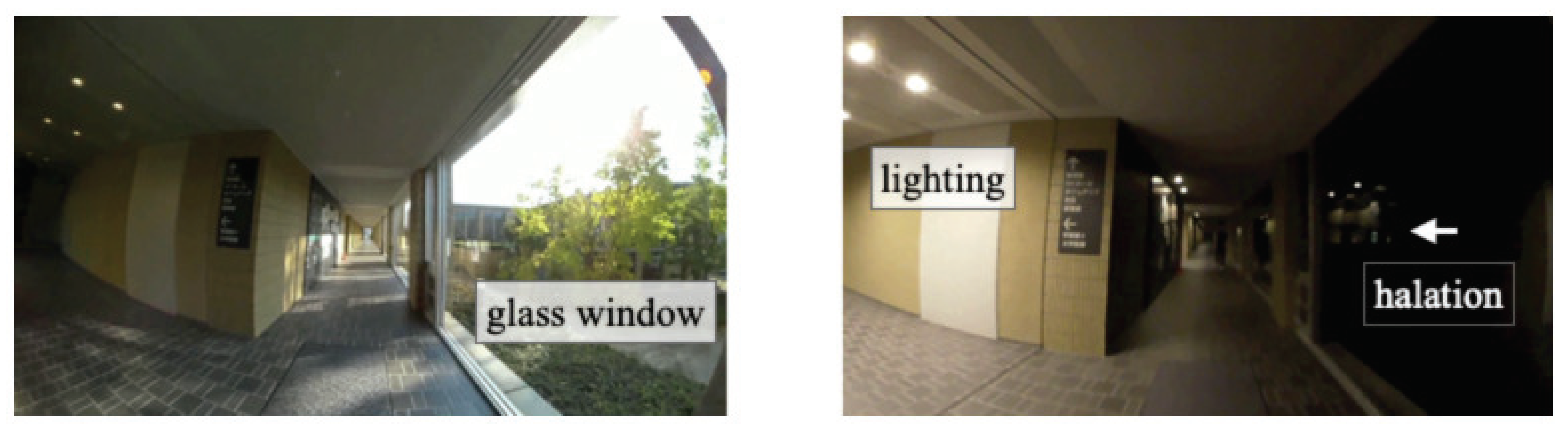
Visual information in indoor images including outdoor features varies considerably in terms of time, weather, and season.
Figure 1 depicts daytime and nighttime scene images in the same position. A great difference arises because of effects from the outside through a transparent glass window. Scene recognition studies using a mobile robot are used in a few cases for accuracy comparison in visual information changes at similar positions. The partial occlusion, corruption, and distortion caused by a limited field of view (FOV) of a camera occur frequently everywhere, depending not only on environmental changes but also on locomotion paths with avoidance of static and dynamic obstacles [
31]. Evaluation criteria and benchmark datasets for these requirements are under development.
For our earlier study [
32], we proposed a unified method for extracting, characterizing, and recognizing VLs that were robust to human occlusion in a real environment in which robots coexist with people. Based on classically established machine-learning (ML) technologies, our earlier method [
32] comprised the following five procedures: VL extraction from generic objects using a saliency map (SM) [
33]; part-based feature description using accelerated KAZE (AKAZE) [
34]; human region extraction using histograms of oriented gradients (HOGs) [
35]; codebook creation using self-organizing maps (SOMs) [
36]; and positional scene recognition using counter propagation networks (CPNs) [
37]. The contributions of this study are the following.
We strove to evaluate the robustness of our improved semantic scene recognition method for extending environmental changes using novel datasets.
We develop our original scene recognition benchmark datasets in which indoor–outdoor visual features coexist.
We evaluate the effects of outdoor features for indoor scene recognition for weather and seasonal changes outdoors.
We evaluate details and quantitative evaluation for visualizing classification results obtained using category maps.
The rest of the paper is structured as follows. In
Section 2, we present our proposed method based on computer vision and machine-learning algorithms of several types.
Section 3 presents our original benchmark datasets of time-series scene images obtained using a wide FOV camera mounted on a mobile robot in an indoor environment surrounded by transparent glass walls and windows for two directions in three seasons. Subsequently,
Section 4 presents evaluation experimentally obtained results of the performance and characteristics of meta-parameter optimization, mapping characteristics to category maps, and recognition accuracy. Finally,
Section 5 concludes and highlights future work. Herein, we had proposed this basic method in the proceeding [
38] ©2018 IEEE. For this paper, we have described detailed results using our novel benchmark datasets.
2. Proposed Method
Our proposed method comprises two modules: a feature-extraction module and a scene recognition module.
Figure 2 and
Figure 3 depict the flow processing and structures of the respective modules. The feature-extraction module performs saliency-based VL extraction and feature description from input images. This module comprises three algorithms: You Only Look Once (YOLO) [
39], SMs [
33], and AKAZE [
34]. First, using YOLO, human regions are extracted from a scene image. Although HOG [
35] was used for our earlier study [
32], the human detection accuracy with HOG, which includes insufficient robustness to rotation and scaling, was increased by only 60%. For this study, we extract bounding boxes (BBs) that include pedestrians using YOLO. We remove feature points inside BBs from VL candidates. Subsequently, salient regions are extracted using SMs [
33]. Finally, features are described using AKAZE from highly salient regions as VLs. Although the feature-extraction module from our earlier study is reused [
32], we introduce YOLO for the novelty of this method.
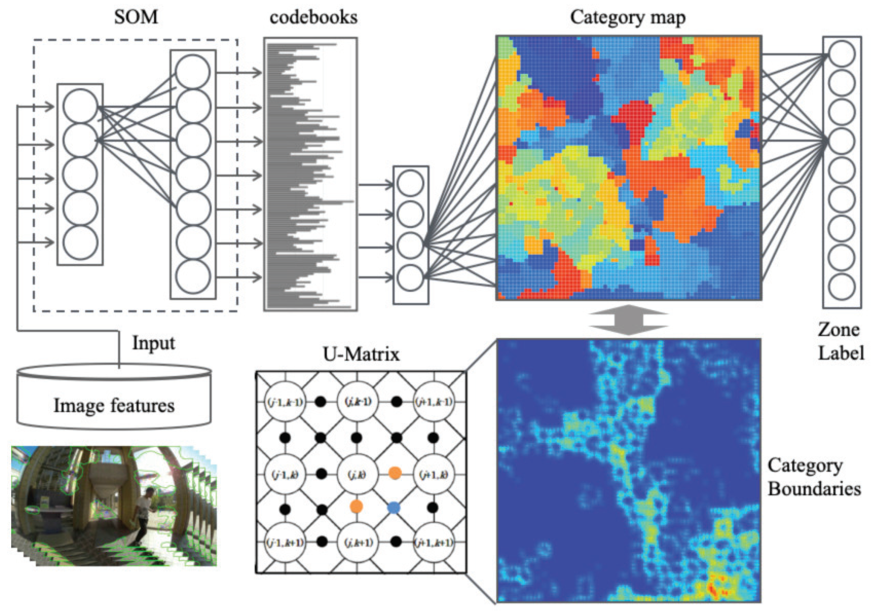
Thereafter, positions are recognized as zones from scene images with the recognition module, as depicted in
Figure 3. The recognition module comprises three algorithms: SOMs [
36], CPNs [
37], and U-Matrix [
40]. Input features are compressed with SOMs for a unified dimension as codebooks. The CPN learning phase performs category map generation and visualization of the similarity of codebooks. The CPN verification phase recognizes scene images as zones using category maps for verification scene images. Moreover, with reference to another earlier method [
41], we use U-Matrix [
40] to extract cluster boundaries from weights on category maps. Cluster boundaries are enhanced for differences between labels and weights. Features and properties of these five algorithms are explained below.
2.1. VL Extraction Using SM
Human stereo vision [
42] provides numerous and diverse real-world information [
43]. Although various decisions are made based on visual information, the speed of processing visual information is rather slow because the amounts of information are large compared to those provided by tactile, auditory, and olfactory senses. Therefore, we have limitations on the use of all visual information for recognition and decision-making. In contrast, we have a mechanism to devote attention solely to some things that should be noticed. Actually, SMs were developed as a mechanism for finding objects that must command attention.
After appending return suppression in similar frames, as a novel application for this study, we extend SMs, which are based on processing for a single image, to time-series images. In addition, recovery was strengthened between consecutive frames for steady VL detection. The brief procedures of saliency maps include the following five steps. First, a pyramid image is created from codebooks for use as input data. Second, a Gaussian filter is applied to the pyramid image. Third, images of the respective components of color phase, brightness, and direction are created. Fourth, feature maps (FMs) are created as visual features of the respective components with center-surround and normalization operations. Finally, saliency maps are obtained from a winner-take-all (WTA) competition for the linear summation of FMs.
2.2. Feature Description Using AKAZE
For conventional generic object recognition, scale-invariant feature transform (SIFT) [
44], SURF [
45], binary robust independent elementary features (BRIEF) [
46], and oriented features from accelerated segment test (FAST) and rotated BRIEF (ORB) [
47] descriptors have been used widely as outstanding descriptors of local features.
Table 1 summerizes feature dimensions in respective descriptors. Actually, SIFT descriptors are robust for rotation, scale, position, and brightness changes, not only from static images but also from dynamic images. Alcantarilla et al. [
48] proposed KAZE using nonlinear scale-space filtering as a feature intended to exceed the SIFT performance. Moreover, they proposed AKAZE [
34], which accelerated the KAZE construction. In contrast to SIFT, AKAZE was demonstrated as being approximately three times faster, although maintaining equivalent performance and accuracy. Therefore, we use AKAZE, which is suitable for indoor environments where environmental changes occurred frequently.
To achieve acceleration of feature detection, AKAZE employs fast explicit diffusion (FED) [
49], which is embedded in a pyramidal framework in nonlinear scale-space filters. Comparison with additive operator splitting [
50] schemes used in their former descriptor KAZE [
48] shows that FED schemes are more accurate. They also provide extremely easy implementation. Moreover, AKAZE introduced a highly efficient Modified-Local Difference Binary descriptor [
51] to preserve low computational demand and storage requirements. The numbers of features points differ in the respective images. Letting
be a set of AKAZE features points, then each feature point includes 64-dimensional feature vectors.
2.3. Human Detection Using YOLO
Based on deep learning (DL) mechanisms [
52], YOLO was proposed by Redmon et al. [
39] as a real-time algorithm for object detection and class recognition. For performing both functions, YOLO is used widely for general object detection of various applications [
53] such as pedestrians [
54], cars [
55], license plates [
56], and accidents [
57]. Moreover, YOLO performs high recognition accuracy and rapid processing speed compared with the single-shot multi-box detector [
58]. Therefore, we used YOLO for human detection instead of HOG [
35], which was used in our earlier study [
32]. However, to keep accuracy in different shapes of human figures in terms of stand up, sitting, lying, and occluded body parts is important. We consider that this is a challenging task for our method combined with YOLO and OpenPose [
59], which is an approach to efficiently detect the 2D pose of multiple people in an image.
The procedures necessary for YOLO are the following. First, the original image is resized into a square. Then the object is detected using a BB. Subsequently, divided grids perform object class and BB extraction in parallel for each region. Finally, the integration result in of both realizes another class of object recognition.
YOLO learns the surrounding context because the entire image is targeted for learning. This mechanism suppresses false detection in background areas. However, divided grids are limited to a fixed size. Moreover, YOLO has a restriction by which the detected objects in each grid can be as many as two because only a single class can be used for identification in each grid. As a shortcoming, the small objects included in each grid degrade the detection accuracy. Generic object detection is beyond the scope of this study. We intend to assess the accuracy of positional scene recognition from scene images with occlusion or deficiency.
2.4. Codebook Description Using SOM
We use SOMs [
36] to create codebooks from AKAZE features. Let
represent the output from the input layer unit
p at time
t. As input features,
are appended to
as VL features.
Let
be a weight from
p to mapping layer unit
q at time
t. Herein,
P and
Q respectively denote the total numbers of input layer units and mapping layer units. Before learning,
are initialized randomly. Using the Euclidean distance between
and
, a winner unit
is sought for the following.
A neighborhood region
is set from the center of
as
where
represents the maximum of learning iterations. Subsequently,
in
is updated as
where
is a learning coefficient that decreases according to the learning progress. Herein, at time
, we initialized
with random numbers. After WTA learning, test data are entered into the input layer. A winner unit is used for voting to create a histogram as a codebook:
.
2.5. Scene Recognition Using CPN
We apply CPNs [
37] to category maps from codebooks. For learning CPNs,
are entered as input features to the input layer of CPNs. Let
be output from the input layer unit
r at time
t. Let
be a weight from
r to Kohonen layer unit
s at time
t. Moreover, let
be a weight from Grossberg layer unit
k to Kohonen layer unit
s at time
t. Herein,
R and
Q respectively denote the total numbers of input layer units and Kohonen layer units. Before learning,
are initialized randomly. Using the Euclidean distance between
and
, a winner unit
is sought for the following.
A neighborhood region
is set as the following from the center of
.
In that equation,
stands for the maximum learning iteration. Subsequently,
and
in
are updated as
where
and
are learning coefficients, which decrease along with learning progress. Herein, at time
, we initialized
and
with random numbers.
As a learning result, is used for the input to CNNs. We define this interface as .
2.6. Boundary Extraction Using U-Matrix
We use U-Matrix [
40] to extract boundaries from category maps. Let
and
be a unit index on a 2D category map. Cluster boundaries are extracted from
using U-Matrix. Based on metric distances between weights, U-Matrix visualizes the spatial distribution of categories from the similarity of neighbor units [
40]. On a 2D category map of square grids, a unit has eight neighbor units except for boundary units. Assuming
U as the similarity calculated using U-Matrix, then for the component of the horizontal and vertical directions,
and
are defined as shown below.
For components of the diagonal directions,
are defined as the following.
3. Scene Recognition Benchmark Datasets
We obtained original benchmark datasets to evaluate the fundamental performance, usefulness, and practicality of our proposed method using a mobile robot equipped with a camera. The primary characteristic of this dataset is that a long corridor inside of our university buildings surrounded by numerous transparent glass walls and windows affects outdoor features. For this study, we obtained scene images in three outdoor conditions: daytime in summer, nighttime in autumn, and daytime in winter.
3.1. Mobile Robot and Camera
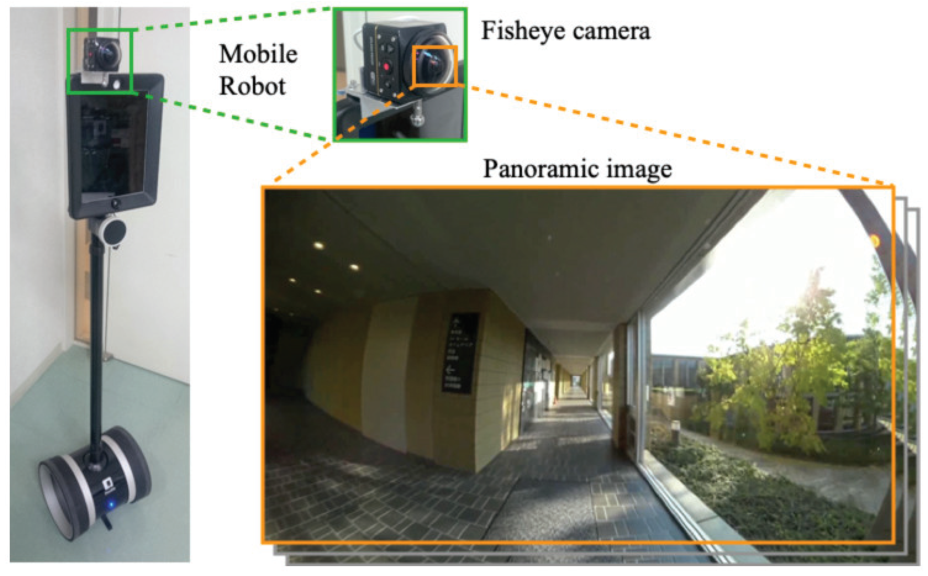
We obtained video sequences using a fisheye lens camera mounted on a mobile robot. We used a two-wheeled inverted-pendulum mobile robot (Double; Double Robotics, Inc. Burlingame, CA, USA). The photograph on the right side of
Figure 4 presents the robot appearance. The robot is 119 cm high with its neck moving up and down to a 31-cm span. For this experiment, we fixed the lowest neck position to maintain constant FOV and locomotion stability.
For our earlier study [
32], we obtained video sequences using a built-in camera of a tablet computer (iPad; Apple Inc. Cupertino, CA, USA).) mounted on the robot head part. The image resolution of
pixels was insufficient to capture objects as VLs. Moreover, the captured video sequences were sent to a laptop using a low-power wireless communication protocol because of a lack of a storage function in the tablet. For this experiment, we used a fisheye lens camera (PIXPRO SP360; Eastman Kodak Co. Rochester, NY, USA).) with high-resolution and wide-range FOV.
Table 2 shows major camera specifications. For this camera, the focal length of the lense is 0.805mm, which is equivalent to a length of 8.25 mm for a 35 mm film. This camera is fundamentally used with a vertical upward arrangement for the lens. We originally developed a camera mount using an L-shaped aluminum plate. Using this mount, we installed the camera at the front of the robot, as depicted in
Figure 4. To ensure good resolution, we used the FOV of the 235-deg mode instead of the 360-deg mode.
3.2. Experimental Environment
Figure 5 presents a photograph and a map of the buildings at Honjo Campus (
N,
E), Akita Prefectural University, Akita, Japan. This campus is located in the countryside. There are three buildings: a lecture building, a common building, and a faculty building. Each building is connected by a crossing corridor. The approximate size of all buildings is 90 m measured longitudinally and 80 m measured laterally.
The total locomotion distance of the robot is 392 m per round. The robot was operated manually using a keyboard on a laptop computer. An operator practiced adequately in advance. The robot moved at a constant speed when obtaining all datasets with no meandering locomotion.
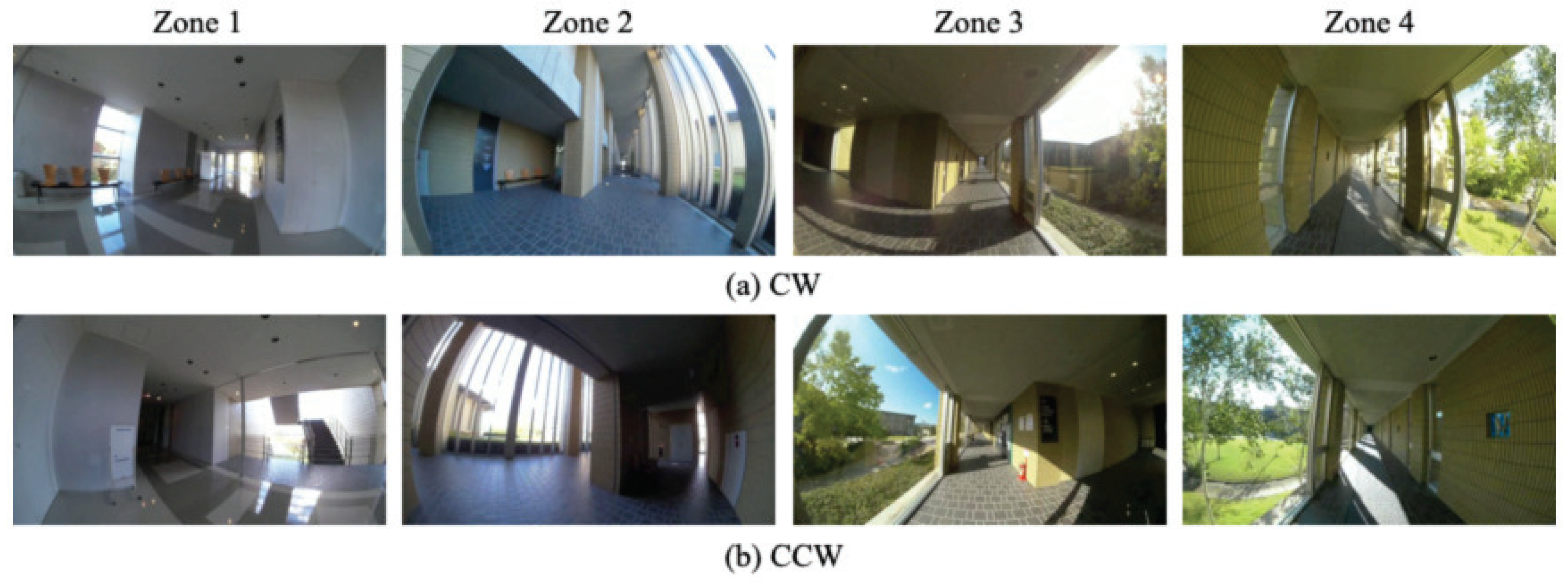
Initially, we divided the route into four zones based on the four right-angle corners, as depicted in
Figure 6a. Subsequently, the respective zones were divided into 2, 4, 8, and 16 refined zones of equal length. As depicted in
Figure 6, 4, 8, 16, 32, and 64 zones were defined for evaluation granularity. We assigned ground truth (GT) labels for five patterns: Zones 1–4, Zones 1–8, Zones 1–16, Zones 1–32, and Zones 1–64.
We obtained video sequences in two directions: clockwise (CW) and counter-clockwise (CCW). The robot moved along the route three rounds in each direction. We obtained six video sequences for one outside condition. Moreover, we conducted experiments to obtain video sequences in three seasons: summer, autumn, and winter. The outside conditions differ among seasons: a summer sunny day in August, a cloudy autumn moonless night in October, and a snowy winter day in December. These weather conditions are typical of this region of northern Japan. For this study, we designated the respective datasets as summer datasets (SD), autumn datasets (AD), and winter datasets (WD).
3.3. Obtained Indoor–Outdoor Mixed Scene Images
For this study, we obtained video sequences using a fish-eye lens camera that was set to the locomotion direction of the robot. The 235-deg FOV provided wide differences in the scene appearances depending on the locomotion direction, even at similar points.
Figure 7 depicts sample images of appearance differences CW and CCW at a similar point. These images indicate that vision-based location recognition is a challenging task of computer vision (CV) studies.
Figure 8 depicts appearance differences of scene images at the same points in the three seasons. High-salience regions and extracted feature points are superimposed on the images with color curves and dots. Feature points on the SD images included various indoor objects in addition to lush trees and lawns outdoors. Moreover, feature points appeared in the buildings through transparent glass walls and windows.
Feature points on AD images included indoor objects in addition to halation from indoor lighting reflected in transparent glass. Images without halation have no feature points. Compared with those of the SD images, the feature points are few. For WD images, the ground surface was covered slightly with snow. Although the sunlight was not intense, the indoor brightness was sufficient to extract object features for VL candidates. Numerous feature points were extracted both indoors and outdoors, similarly to the SD images.
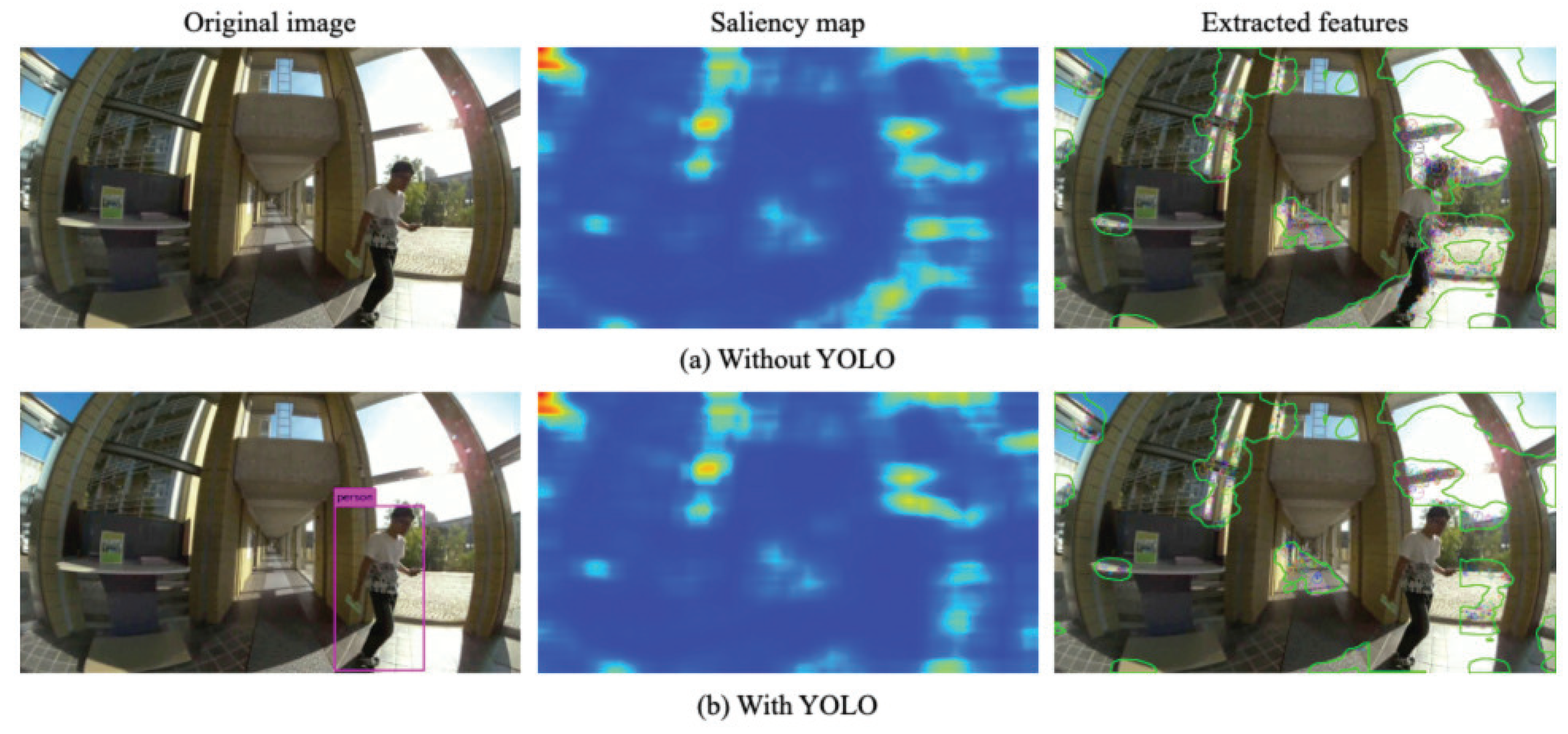
3.4. Extraction of Image Features
Figure 9 depicts comparison results of extracted features. This example image includes a person as a moving object in the left panels. The middle panels depict saliency regions as VL candidates. The right panels depict extracted features from high saliency regions. The feature points are distributed over the person. Using YOLO, the human region is excluded from salient regions. The AKAZE features overlapped on the person disappeared.
4. Evaluation Experiment
4.1. Benchmark and Evaluation Criteria
We conducted an evaluation experiment to develop VL-based positional scene recognition from scene images obtained using a mobile robot.
Table 3 presents details of 18 datasets in each season and the locomotion direction. We used leave-one-out cross-validation [
60] as evaluation criteria. Specifically, a set of datasets in each season and direction was divided into two groups: one dataset was left for validation; the other datasets were used for training. We calculate the respective recognition accuracies for the five patterns of divided zones.
For evaluation criteria, the recognition accuracy
[%] for a validation dataset is defined as
where
and
respectively represent the total numbers of validation images and correct recognition images that matched zone labels as GT.
4.2. Optimization of Parameters
Before the scene recognition evaluation experiment, we conducted a preliminary experiment to optimize meta-parameters for the regulation of our proposed method. The optimization subjects are the following four parameters: S, which is related to expression and granularity and expression of codebooks; Q, which is related to the resolution and expression of category maps; SOM learning iterations; and CPN learning iterations. Herein, the computational cost for the simultaneous optimization of these four parameters is an exponential multiple compared with a single case. Therefore, we optimized them sequentially. For this parameter optimization experiment, we merely used the SD images.
Figure 10 depicts the optimization result of the number of mapping layer units:
S for SOMs and
S for CPNs. We changed
from
to
at
intervals. The optimization experiment results revealed that
improved steadily from
to
. The local maximum of 52.3% was obtained at
, which corresponds to
units. The accuracies were reduced in other unit sizes. Therefore, the optimal size of the SOM mapping layer was ascertained as 128 units.
For CPN, we changed Q from units to units at unit intervals. The optimization experiment results revealed that improved steadily from units to units. The local maximum of 51.1% was obtained at units. Subsequently, dropped to 48.9% at units. Therefore, the optimal size of the CPN mapping layer was ascertained as units.
In addition,
Figure 11 depicts the optimization result of learning iterations for SOMs and CPNs. Herein,
denotes learning iterations. We changed this parameter from
to
at
intervals. The optimization experiment results of SOM learning iterations revealed that
improved steadily according to the greater number of learning iterations. The maximum
% was obtained at 10,000,000 iterations for SOMs.
For CPN learning iterations, improved rapidly up to 1,000,000 iterations. Subsequently, improved gradually according to the greater number of learning iterations. Maximum % was obtained at 100,000,000 iterations. However, the accuracy difference compared with 10,000,000 iterations was only 0.7 percentage points. Moreover, the accuracy difference compared with 1,000,000 iterations was a mere 0.8 percentage points. In addition to those slight differences achieved, the computation time increased exponentially. Therefore, this study showed the optimal CPN learning iterations at 1,000,000 iterations, given reasonable limitations of engineering, with balanced computational costs and accuracy.
4.3. Positional Scene Recognition Results
Figure 12,
Figure 13 and
Figure 14 depict recognition accuracies for the respective datasets as shown in
Table 3. As an overall tendency, the recognition accuracies vary depending on the season and the number of zones. The mean
values of SD, AD, and WD were found, respectively, as 82.4%, 79.1%, and 78.1%. The experimentally obtained results revealed 4.3 percentage point difference in accuracy among the three datasets.
For the locomotion direction for SD, the mean of CW is 1.9 percentage points higher than that of CCW. For AD, the mean of CCW was 2.2 percentage points higher than that of CW. As a similar tendency to that of WD, the mean of CCW was 4.7 percentage points higher than that of CW.
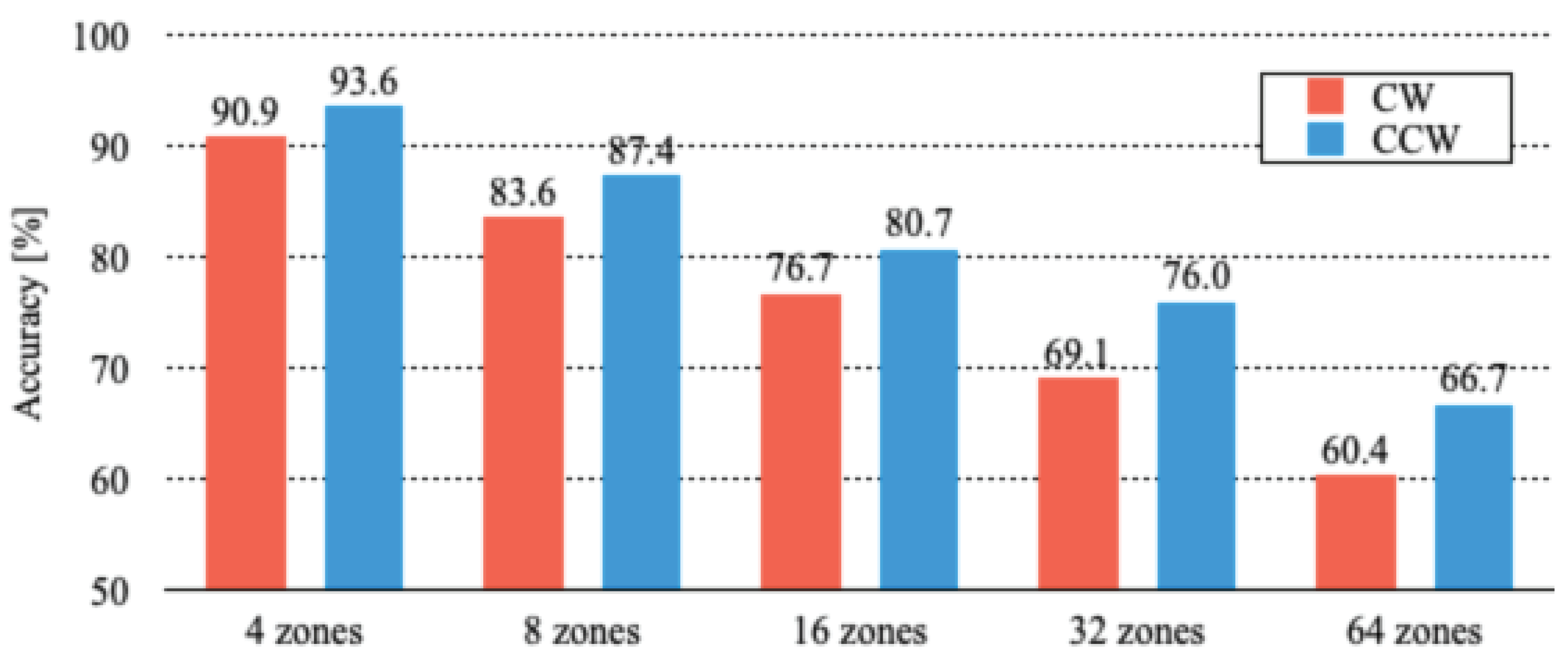
Recognition accuracy decreases according to a greater number of divided zones because of increasingly challenging levels for similar and overlapped images. Although of 64 zones of CW persists to the maximum of 69.3% for SD, is maintained at a minimum of 60.4% for WD. Herein, a single-zone length for the case of 64 divisions with a total path length of 392 m is approximately 6 m. When we subdivide the routes, we extract more information that is normally found in time series. However, our proposed method includes no mechanism to extract time-series features due to no recurrent structure. Therefore, the recognition accuracies were decreased according to the increased number of divided zones. Regarding seasonal changes, we assumed that AD images would have fewer outdoor features and improved recognition accuracy because of the fall of leaves on trees, as opposed to SD images. Similarly, we assumed that the WD images would be further improved by the snowfall. Although the overall recognition accuracy varies with the season, the experimentally obtained results revealed no contribute to the reduction of the decline as the number of zones increases. On the other hand, the results revealed that our proposed method provided of more than 60% with a resolution of 6 m for a monotonous indoor environment such as this corridor, which is greatly affected by the outdoors. That result was achieved solely using visual information obtained using a monocular camera with no GNSS or odometry.
4.4. Analysis and Discussion
We analyzed detailed recognition results in each zone using a confusion matrix. For this experiment, we visualized the whole tendency of recognition results obtained using a heatmap because the maximum division is 64 zones.
Figure 15 depicts confusion matrixes using a heatmap. We designate it as a heatmap confusion matrix (HCM), which can check all zone results at a glance.
In HCMs, correct results are distributed diagonally from the upper left to the lower right. A high color temperature result of this diagonal line represents high recognition accuracy. The distribution of higher color temperature distant from the diagonal line represents false recognition. Therefore, the HCM displays correct recognition as a high color temperature and false recognition as a low color temperature
For all HCMs, as depicted in
Figure 15, we integrated CW and CCW results because we evaluated the difference of the locomotion direction, as depicted in
Figure 12,
Figure 13 and
Figure 14. The experimentally obtained HCMs revealed that a greater number of zone divisions corresponds to decreased diagonal color temperature. Nevertheless, no distribution of false recognition resembling hot spots, diffused false recognition appeared overall. In three datasets associated with different seasons, SD achieved the highest recognition accuracy.
Particularly,
Figure 16 depicts the results of 16 zones in SD. For this result, Zones 1–4 and Zones 13–16 show high accuracy. In contrast, false recognition occurred in Zones 5–12. Particularly, numerous instances of false recognition occurred in Zones 6 and 12. The left panel of
Figure 16 depicts images in Zones 1–4 with high accuracy. The path along which the robot moved in the corridor surrounded by lecture rooms has a small effect from outdoors. The right panel depicts images in Zones 9–12 with low accuracy. The scenes surrounded by transparent glass walls and windows of both sides exhibit a strong effect from outdoors.
As a benefit of our proposed method, the relation between zones can be visualized as a similarity in a low-dimensional space using a category map that is generated through learning based on competition and the neighborhood.
Figure 17 depicts category maps created as learning results for the respective seasonal datasets. Each column of the figure depicts the category maps for which the number of divided routes is changed from 4 zones to 64 zones. The heatmap bars presented on the right side of each category map are divided according to the total number of divided zones. Clusters are created on a category map from similarities among categories. By contrast, complex features with inconsistent relations are distributed in multiple small clusters. The respective category maps demonstrated that clusters are distributed at multiple locations. This distribution property suggests the complexity of image features in each zone in VL-based semantic positional scene recognition.
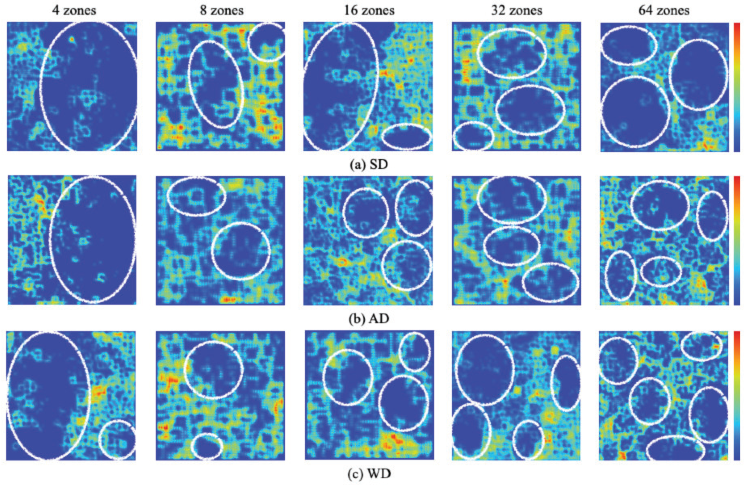
For analysis of mapping properties of category maps, we used U-Matrix to extract cluster boundaries. Based on distances among weights on a category map, U-Matrix extracted similarity of neighbor units. We visualized boundary depths using a heatmap. Low similarity weights, which are also regarded as having low similarity between units, are displayed for lower color temperatures. In contrast, high similarity weights, which are considered to have high similarity among units, are displayed for higher color temperatures.
Figure 18 depicts extraction results of cluster boundaries obtained using U-Matrix for all datasets of the respective divided zones. The white circles depict independent clusters that are surrounded by boundaries as high temperatures. Ideally, a suitable model comprises boundaries with low color temperatures inside clusters and high temperatures outside clusters. In this case, clear boundaries are obtained on a category map. Such a model is derived from highly independent feature distributions in a scene image. Nevertheless, scene appearances include similar and contradictory features for zones that are divided evenly along with the locomotion path, as depicted in
Figure 6. Therefore, U-Matrix provided no distribution clusters according to the number of zones, similar to the results of category maps. The tendency obtained from this experimentally obtained result demonstrated that the clusters changed from a large cluster to a small cluster on U-Matrix for the number of zone increases. Our method handled the difficulty by which sets for dividing a scene are more complicated and difficult.
Rapidly progressed DL networks have been applied to various challenges posed by CV and RV. Our method, which used YOLO [
39] to some degree, showed benefits from advanced DL performance. Dramatic improvement of recognition accuracy is expected to be sufficient using DL networks for the feature-extraction module for preprocessing and for the recognition module for recognition. Based on our earlier study [
32], this study was aimed at developing original indoor benchmark datasets that include numerous transparent glass walls and windows to evaluate robustness for environmental changes outdoors. Our method was developed using classical ML-based algorithms without using DL because we visualized relations and similarities of scene images using category maps and U-Matrix for zone-based positional recognition with several granularity types.
For application to different purposes and benchmarks, we replaced the ML with a DL recognition module in our earlier study [
41]. We then demonstrated the accuracy and computational cost differences between DL and ML. Actually, CV algorithms require both offline batch processing and online real-time processing. By contrast, RV algorithms fundamentally require online real-time processing from limited computational resources, especially for small robots including drones. Technological development and evolution related to cutting-edge AI devices [
61] are expected to improve the shortcomings related to computational costs for DL algorithms. As a present optimal solution, we used ML algorithms with efficiency for current robots with no computational enhancement. The recognition module can be replaced with DL if accuracy is the highest priority for a target system. The input interface for this case can be set to the feature-extraction module but also directly to the recognition module. In consideration of such a replacement, we divided our proposed method into two independent modules.
5. Conclusions
This paper presented a vision-based positional scene recognition method for an autonomous mobile robot using visual landmarks in an actual environment of coexisting humans and robots. We developed original benchmark datasets that include indoor–outdoor visual features in environments surrounded by transparent glass walls and windows. To include various and diverse changes of scene appearances, the datasets include two locomotion directions and three seasons. We conducted evaluation experiments for VL-based location recognition using datasets of time-series scene images obtained from a wide FOV camera mounted on a robot that ran a 392 m route that was divided into 64 zones with fixed intervals. We verified the performance and characteristics of meta-parameter optimization, mapping characteristics to category maps, and GT-based recognition accuracy. Moreover, we visualized similarity between scene images using category maps. We also visualized the relation of weights using U-Matrix.
As a subject of future work, we expect to introduce Elman-type feedback neural networks combined with deep learning mechanisms as a framework for learning time-series feature changes. We expect to extract flexible and variable zones based on visual changes obtained from category maps and U-Matrix. Moreover, we expect to implement our proposed method as online processing instead of the current offline processing for applying human-symbiotic robots of various types and various environments. Furthermore, we would like to open all the images as a novel open benchmark dataset after inserting semantic information including segmentation, recognition, labeling, GT, annotations, and security and privacy treatment.


