Multi-Robot Coverage and Persistent Monitoring in Sensing-Constrained Environments

Abstract

This article examines the problems of multi-robot coverage and persistent monitoring of regions of interest with limited sensing robots. A group of robots, each equipped with only contact sensors and a clock, execute a simple trajectory by repeatedly moving straight and then bouncing at perimeter boundaries by rotating in place. We introduce an approach by finding a joint trajectory for multiple robots to cover a given environment and generating cycles for the robots to persistently monitor the target regions in the environment. From a given initial configuration, our approach iteratively finds the joint trajectory of all the robots that covers the entire environment. Our approach also computes periodic trajectories of all the robots for monitoring of some regions, where trajectories overlap but do not involve robot-robot collisions. We present experimental results from multiple simulations and physical experiments demonstrating the practical utility of our approach.

1. Introduction

A mobile robot equipped with few sensors can be programmed to bounce off walls in a predictable way. Though a simple, predictable bouncing behavior can be easily modeled and trivially implemented, is it useful? We answer in the affirmative from two perspectives: First, from a practical point of view, most robots are designed to solve specific problems (for example, to vacuum floors). Manufacturers of robots for cost-conscious consumers produce fairly parsimonious devices with regard to sensing and actuation. Second, more theoretically, within the robotics research community, there is a long line of research dealing with limited sensing robots that aims to identify the resources necessary to carry out some tasks; these research seek to advance understanding of the tasks themselves, determine minimal resource footprints, and to develop theory to aid understanding the design of robots.

Furthermore, compared to single robots, multiple robot systems have the potential to vastly improve (or speed-up) performance in important applications, such as search and rescue, surveillance, intrusion detection, environmental monitoring, vacuum cleaning, lawn-mowing, mine sweeping, exploration, automated farming, and painting. All of these are instances of the two abstract problems that are the focus of this article: (i) multi-robot area coverage — the problem of visiting all locations within an environment using a team of mobile robots by introducing techniques to achieve greater scalability and ameliorate the curse of dimensionality; (ii) persistent monitoring — The problem of planning and executing trajectories for multiple robots to visit a known set of regions of interest continually in an environment by finding solutions which ensure that the robots’ motions are collision-free (a form of implicit coordination).

In both problems studied in this article, multiple robots move concurrently and execute a simple bouncing behavior: the robots move straight until they discover walls by driving into them, or they collide with each other while covering the environment; they then rotate (with respect to their current motion) counterclockwise by some angle. The motion is, thus, parameterized by a set of rotation angles, which we term bouncing angles. This motion model enables the construction of trajectories for the robots that cover the environment and also monitor a subset of regions in the environment for an extended period of time. Most importantly, the examined bouncing behavior is easy to implement in mobile robots. Our approach not only applies to bouncing robots but also will work for any robots that have a consistent dynamics since it exploits the natural dynamics of the system and uses actions sparingly. We have applied this approach for finding the long-term behavior of a specific type of underwater vehicles called drifters [1]. Interestingly, the bouncing behavior has recently been used in aerial robot swarms [2] and in micro-robots [3], where computation and sensing are limited.

These motions can be executed by limited sensing robots equipped with known sensors, and we are interested in solving a breadth of problems in polygonal environments, possibly with obstacles, for such robots. An example scenario of an indoor environment is illustrated in Figure 1, where multiple limited sensing robots move through the environment. Additionally, although sensors are available with lower costs now, the overuse of sensors requires powerful computation systems and abundant memory inside sophisticated robots. Instead, we use small-brained robots that can feed minimal sensor outputs directly to motors.

This research falls within the broader context of control and sensing with limited (or even minimal) sensing robots. Several researchers have examined minimal sensing robots to solve different tasks such as localization [4,5,6,7], navigation [8,9,10,11], micromanipulation [3] and mapping [12]. More recently, bouncing strategies for a single robot have been carefully analyzed, and closed-form solutions have been found for simple polygonal environments [13] and polygonal environments with obstacles when nondeterministic uncertainty is considered in the bouncing robot’s motion [14]. These work, along with our own, avoid robots with extensive sensory, computational, and memory capabilities, motivated both pragmatically—to reduce costs and energy consumption for the individual robots, and theoretically—to reduce the conditions known to be sufficient for the task performance. In particular, the approach in this article uses robots equipped with only a clock and contact sensors.

Though our results show that the considered problems can be effectively tackled with limited sensing robots for known rectilinear environments, we emphasize that coverage of an area is a challenging problem: finding a path of optimal length for a given region is NP-hard (via reduction to the Traveling Salesman Problem [15]). Therefore, heuristic solutions are presented in Reference [16] to provide the complete area coverage of a known environment with multiple robots. Even the best zig-zag motion-based and boustrophedon motion-based [17] coverage solutions typically require robots to follow paths using feedback from powerful (and hence expensive) sensors.

Further, we consider weighted instances of the problem in which some regions of the environment are more important than others and highly-weighted regions must be visited more frequently than lower-weighted ones in long-term monitoring. In such cases, the generation of trajectories is challenging because it is not straightforward to find collision-free trajectories of the robots when the robot’s paths must necessarily overlap. Our work in monitoring addresses the robot-robot collision avoidance problem in the overlapping trajectories of robots based on their initial configurations rather than their stopping policies [18].

In our previous work, we use simple cell-to-cell mapping (SCM) [19], a deterministic dynamical system method, for solving the localization task [5] and the navigation task [9] utilizing a single bouncing robot. In this article, we extend the same SCM method to tackle the coverage and persistent monitoring tasks in multi-robot settings. This dynamical system perspective is motivated by the general concepts of limit cycles and basins of attraction, used in control theory [20] and control of robots with sophisticated dynamics [21].

This article makes the following contributions:

• We propose an approach using simple cell-to-cell mapping [19] to find a joint trajectory of multiple bouncing robots for covering a known environment.
• We also present an algorithm to generate the collision-free and overlapping trajectories of multiple robots that monitor some regions of interest in an environment persistently.

Parts of this article were included in the corresponding author’s doctoral dissertation [22]. This article solves one more problem in multi-robot settings and presents its method and experimental evaluation, in addition to other refinements and corrections.

The remainder of the article is structured as follows—Section 2 presents the related literature. In Section 3, we account for the motion model of multiple robots and the fundamentals of cell-to-cell mapping, and then formulate the problems we are interested in. In Section 4, we describe our approach for solving the formulated problems in detail. Then, we outline the implementation of our approach with simulation results and physical experiments in Section 5. Finally, we conclude the article in Section 6 with the discussion.

2. Related Work

This section discusses the literature relevant to the problems considered, especially those using limited sensing robots.

2.1. Coverage

The problem of coverage by multiple robots has been investigated in many different studies. One survey on coverage path planning [23] studied approaches that are evaluated based on whether they can be used online or offline, and on the type of environments they can handle. In Reference [24], the authors propose the fast coverage of the environment based on the unpredictable trajectory of a mobile robot with the use of a Logistic map, and provide a chaotic random bit generator for a time-ordered succession of future robot locations. Because of the obstacle avoidance technique used in this work, robots did not cover the free space around obstacles nor the boundary of the environment. In our work, robots cover the boundary of a given area.

Gabriely and Rimon [25] proposed a spanning-tree based coverage algorithm for a single robot. This work was extended for multi-robot coverage as a multi-robot spanning-tree based coverage algorithm in References [26,27], and as a multi-robot forest coverage algorithm in Reference [28]. These multi-robot coverage algorithms are either centralized or require reliable communication between robots and depend on extensive broadcast messages. The computational and memory complexities for handling the sensor information of this kind of system are very high. Our bouncing robots do not communicate with each other for covering an area.

A recent offline spanning-based tree multi-robot coverage method presented by Fazli et al. [29] deals with the case where the robots have a limited visibility range. This approach is also shown to be complete and robust with regard to robot failure. In Reference [30], the authors designed the multi-robot repeated area coverage as the Multiple Traveling Salesman Problem and proposed three distributed cluster-based algorithms. Fazli and Mackworth [31] also proposed the repeated coverage of the boundaries of a target area and the structures inside it by multiple robots with limited visual and communication range. We do not use any visual sensing or communication medium in our robots. Instead, we address the coverage problem using the simple bouncing behavior of multiple robots.

2.2. Persistent Monitoring

The collision avoidance of multiple robots with limited sensing capabilities in the persistent monitoring task is challenging. In the literature, a number of collision avoidance methods have been proposed for solving the considered task. In References [32,33], Smith et al. developed methods for computing closed monitoring trajectories for robots, and for computing the speed with which each robot should follow its trajectory. In the more closely related work in Reference [18], a solution to multi-robot persistent monitoring, where robots have intersecting trajectories, was proposed. They developed a collision avoidance procedure based on stopping policies while the robots follow their trajectories. In these papers, multiple robots have to control their speeds using their prescribed speed profiles to avoid collisions or follow their trajectories, whereas our robots maintain a fixed speed and they move continuously without stopping.

Lan and Schwager proposed an incremental sampling-based algorithm to plan a periodic trajectory for a single robot that is suitable for persistent monitoring [34]. Yu et al. model the planning of informative tours for the persistent monitoring of a spatiotemporal field with time-invariant spatial correlations using autonomous mobile robots [35]. The coordination of the motions of multiple robots’ trajectories for avoiding collisions is presented in Reference [36]. On the other hand, an approach is proposed for smooth and collision-free navigation of multiple mobile robots amongst each other in a shared environment [37]. An optimal control approach for solving the multi-agent persistent monitoring task is developed in Reference [38], where the objective is to control the movement of multiple cooperating agents to minimize an uncertainty metric in a given mission space. In our work, we find all the periodic cycles based overlapping trajectories of multiple robots that monitor a subset of regions in a known environment and also avoid robot–robot collisions in these trajectories without doing any speed control of robots.

3. Preliminaries

This section defines the motion model of multiple robots, explains cell-to-cell mapping with required notations, and formulates the problems we will solve in our work.

3.1. Motion Model

We model multiple differential drive mobile robots as point robots which share a common 2D workspace, $\mathcal{W}={\mathbb{R}}^2$, and a collection of static obstacles composing an obstacle region, $\mathcal{O}\subset \mathcal{W}$, where each element in $\mathcal{O}=\{{\mathcal{O}}_1,{\mathcal{O}}_2,\cdots ,{\mathcal{O}}_k\}$ is modeled as a polygon. Each robot is equipped with only contact sensors and a clock. The speed of all robots is fixed. The free space for each robot is denoted by the environment $E=\mathcal{W}\setminus \mathcal{O}$, where each robot can move in the E avoiding collisions with both the static obstacles and other robots. Let $\partial E\subset E$ be the boundary of E. We consider that each robot knows the map of the environment and its initial configuration. Let the set of bouncing angles for all robots be $\Phi$ by which they can rotate reliably. This is important to note that it is not easy to measure the bouncing angle accurately using inexpensive differential drive robots. However, we are able to measure some bouncing angles reliably and accurately using such robots in our physical experiments (see Section 5).

All robots move straight in the environment at the same time until they bump into the boundary of the environment $\partial E$ or collide with each other (in solving the coverage task only), as illustrated in Figure 2. Once a robot’s contact sensor detects a bump, it rotates counterclockwise with a specified bouncing angle $\varphi \in \Phi$ from its current orientation by commanding a constant angular velocity and using a clock to rotate for some fixed period. Thereafter, if it faces free space, it travels forward again and repeats this simple behavior.

3.2. Cell-to-Cell Mapping

We consider that there are m robots, ${\mathcal{A}}^1,{\mathcal{A}}^2,\cdots ,{\mathcal{A}}^m$. Each robot, ${\mathcal{A}}^i$, has its associated configuration space $X^i=E\times S^1$, where $S^1$ is the set of directions in the unit circle that represents the robot’s orientations. The configuration spaces of all robots have the same dimension. Let $x^i\in X^i$ represent the configuration of each robot, where $x^i=(x_t^i,y_t^i,{\theta }^i$), $(x_t^i,y_t^i)$ is the corresponding robot’s position, and ${\theta }^i$ is its orientation. A physical configuration space is defined as the configurations of all robots simultaneously, $X=X^1\times X^2\times \cdots \times X^m$. A configuration $x\in X$ specifies all robot configurations.

There are two sources of obstacle regions in the configuration space: (1) robot–obstacle collisions and (2) robot–robot collisions [39]. The robot-obstacle collision, $X_{\mathrm{obs}}^i\in X$, for each robot ${\mathcal{A}}^i$, where $1\le i\le m$, that collides with the obstacle region $\mathcal{O}$ is defined as:

$$X_{\mathrm{obs}}^i=\{x\in X|{\mathcal{A}}^i\left(x^i\right)\cap \mathcal{O}\ne \varnothing \}.$$

(1)

The robot–robot collision, $X_{\mathrm{obs}}^{ij}\in X$, between each pair of robots ${\mathcal{A}}^i$ and ${\mathcal{A}}^j$ is defined as:

$$X_{\mathrm{obs}}^{ij}=\{x\in X|{\mathcal{A}}^i\left(x^i\right)\cap {\mathcal{A}}^j\left(x^j\right)\ne \varnothing \}.$$

(2)

Thus, the entire obstacle region in X is:

$$X_{\mathrm{obs}}=\left(\bigcup _{i=1}^m{X}_{\mathrm{obs}}^i\right)\bigcup \left(\bigcup _{ij,i\ne j}{X}_{\mathrm{obs}}^{ij}\right).$$

(3)

The free configuration space $X_{\mathrm{free}}=X\setminus X_{\mathrm{obs}}$. Taking the configurations of all robots into account, each configuration $x\in X_{free}$ is a $3m$-dimensional vector and $x=(x_t^1,y_t^1,{\theta }^1,\cdots ,x_t^m,y_t^m,{\theta }^m)$. Hence, we discretize the free configuration space $X_{\mathrm{free}}$ into $3m$-dimensional cells. This discretized configuration space is called the cell state space. Let N be the total number of cells. Thus, the free configuration space of the system $X_{\mathrm{free}}$ is described by a cell index $z\in \{1,\dots ,N\}$. Let $Z=\{1,\dots ,N\}$ denote the collection of $3m$-dimensional cells.

The system dynamics can be explained as a series of cells by finding the system’s state at discrete times. Let $e\left(k\right)$ be the cell describing the state of the system at $t=k\Delta t$, $k=0,1,\dots$ with $\Delta t$ being the time between two state inspections. In the deterministic case, the system dynamics of the cell-to-cell mapping are described as

$$e(k+1)=\mathcal{C}\left(e\right(k\left)\right).$$

(4)

The above system evolution $\mathcal{C}:\mathbb{N}\to \mathbb{N}$ is called a SCM [20] in the cell state space. In this mapping, the next state of the system is dependent on only its current state instead of the mapping step k.

For a clear understanding of our approach, we present some pertinent definitions of the cell-to-cell mapping method [20,40].

Definition 1.

(Periodic Cell) A cell z satisfying $z={\mathcal{C}}^k\left(z\right)$, for some $k\in \mathbb{N}$, is called a periodic cell with a period of k.

Definition 2.

(Transient Cell) A cell that is not periodic is called a transient cell and it maps into a periodic cell in a finite number of steps.

Definition 3.

(Periodic Group) A sequence of K distinct cells $e\left(j\right)$, where $j=1,2,\dots ,K-1$, which satisfies

$$\begin{array}{cc}\hfill e(j+1)& ={\mathcal{C}}^j\left(e\left(1\right)\right),j=1,2,\dots ,K-1\hfill \\ \hfill e\left(1\right)& ={\mathcal{C}}^K\left(e\left(1\right)\right),\hfill \end{array}$$

(5)

is called a periodic group with a period K and each of the cells $e(·)$ is said to be a periodic cell with the period K. This periodic group is also called an attractor or a limit cycle.

Definition 4.

(Transient Trajectory) A transient trajectory is the set of initial cells that are finally leading to a particular periodic group (attractor). The collection of transient trajectories is called abasin of a ttraction.

3.3. Problem Formulation

We define a finite action space U, which is a set of all possible actions $u\in U$ that a robot can perform. The robot records the angle of rotation $\varphi \in \Phi$ when it bumps and then rotates. The robot also records $\left\{0\right\}$ as its one step forward movement when it moves straight for a specific period. Therefore, the action space is $U=\left\{0\right\}\cup \Phi$.

In our first problem of interest, we take advantage of robot-robot collisions to tackle the coverage problem utilizing multiple bouncing robots. We assume that the robots’ initial configurations are known. Let $x_0\in X_{\mathrm{free}}$ be the initial configuration of m robots, where $m>=2$. The initial configuration of m robots is the initial cell from which we apply the cell-to-cell mapping. Then, the state of the system evolves over time and creates a joint trajectory for these robots. Let $T=[0,\infty )$ be a time interval of the execution of the system. We define a joint trajectory of m robots as $\tilde{x}:[0,T]\to X_{\mathrm{free}}$ with $\tilde{x}\left(0\right)=x_0$ and where $\tilde{x}\left(t\right)$ represents the state of the system at time t. The joint trajectory of all the robots will end up in a cyclic trajectory according to the properties of the system evolution of the SCM [20]. Therefore, we are interested in finding a joint trajectory of m robots that attempts to cover the environment. This motivates us to define the coverage problem for multiple robots as follows:

Problem 1.

Finding a joint trajectory of multiple robots for covering an environment: Given an environment E, a set of bouncing angles Φ for m robots, and an initial configuration of m robots $x_0$, find a joint trajectory $\tilde{x}$ of m robots that attempts to cover the given environment E.

Our second problem of interest is to solve the multi-robot monitoring problem. For instance, we want to monitor some target regions of interest in an environment for a long period of time. We can find trajectories of m robots that cover m regions. Let $F_j\subset E$ be a target region in the environment E and $F={\bigcup }_{j=1}^m{F}_j$ be the set of all target regions. We consider that these trajectories may be overlapping and robots have to avoid collisions among them. In this scenario, we formulate the persistent monitoring problem as follows:

Problem 2.

Generating trajectories of multiple robots for monitoring a set of environment regions: Given an environment E, a set of target regions in the environment $F\subset E$, and a set of bouncing angles Φ for m robots, generate collision-free and distributed trajectories of m robots that persistently monitor F.

4. Approach

In this section, we describe our approach for solving the two problems formulated in Section 3 in detail.

4.1. Finding a Joint Trajectory of Multiple Robots for Coverage

In our approach, we find a joint trajectory $\tilde{x}$ of m robots starting from a random initial configuration (cell) $x_0$ to cover the environment E. These m robots use their respective bouncing angles from the given set of bouncing angles $\Phi$ once they collide with each other or against the boundary of the environment $\partial E$. In this context, we extend the SCM method in the high-dimensional configuration space of multiple robots.

To find the joint trajectory $\tilde{x}$, Algorithm 1 takes as input the environment E, the initial configuration $x_0$, and the set of bouncing angles $\Phi$ for m robots, and generates as output the joint trajectory $\tilde{x}$ that the robots follow to cover the environment.

In Algorithm 1, all cells are initially unprocessed cells. First, a cell b is calculated from the known initial configuration $x_0$ and added to the trajectory $\tilde{x}$ as the initial cell (lines 2–3). Then, we apply the SCM to create a cell sequence that is a part of the trajectory. For l iterations, the cell sequence $z,\mathcal{C}\left(z\right),{\mathcal{C}}^2\left(z\right),\cdots ,{\mathcal{C}}^k\left(z\right)$, where $k\in \mathbb{N}$, is iteratively generated from the initial cell b. In lines 6–12, during the cell sequence generation, all cells are identified as processed cells by assigning the value 1 to these cells. The cell configuration z is calculated from the cell b, which represents the configurations of all m robots $x=(x_z^1,y_z^1,{\theta }_z^1,\cdots ,x_z^m,y_z^m,{\theta }_z^m)$ (line 8). In line 9, the next mapped cell configuration of m robots $z^{\prime }$ after z is calculated as below:

$$\begin{array}{cc}\hfill x_{z^{\prime }}^i& =x_z^i+cos{\theta }_z^i,\hfill \\ \hfill y_{z^{\prime }}^i& =y_z^i+sin{\theta }_z^i,\hfill \\ \hfill {\theta }_{z^{\prime }}^i& =\left\{\begin{array}{cc}{\theta }_z^i,\hfill & \mathrm{if}(x_{z^{\prime }}^i,y_{z^{\prime }}^i)\in X_{\mathrm{free}},\hfill \\ ({\theta }_z^i+{\varphi }_z^i)mod2\pi ,\hfill & \mathrm{otherwise},\hfill \end{array}\right.\hfill \end{array}$$

(6)

where $i\in \{1,\dots ,m\}$. The calculation of the next mapped cell configuration $z^{\prime }$ takes robot-obstacle collisions and robot-robot collisions into account.

This cell-to-cell mapping also finds the next mapped cell of each of the m robots. The cell number of the next mapped cell, $c_b$ is computed from the center locations of all robots and their orientations ($x_{z^{\prime }}^1,y_{z^{\prime }}^1,{\theta }_{z^{\prime }}^1,\cdots ,x_{z^{\prime }}^m,y_{z^{\prime }}^m,{\theta }_{z^{\prime }}^m$) of $z^{\prime }$ (line 10). We add the next cell $c_b$ to the trajectory $\tilde{x}$ as a new cell and the cell transition from b to $c_b$ is made in the trajectory $\tilde{x}$ as a connection or transition (line 11). The next cell b is updated with $c_b$ and the cell configuration z is updated with $z^{\prime }$ (line 12). The cell sequence generation continues as long as the next mapped cell b is an unprocessed cell at each iteration. A generated trajectory $\tilde{x}$ from an initial configuration $x_0$ as an initial cell is illustrated symbolically in Figure 3a, where each square represents a $3m$-dimensional cell of the cell configuration space $X_{\mathrm{free}}$. Some cells of $\tilde{x}$ form a cycle and others lead to this cycle.

Algorithm 1: MultiRobotCoverage ($E,x_0,\Phi$)

Let ${\beta }_l$ be the best unprocessed and nearest neighbor cell of the last cell of the trajectory $\tilde{x}$ at the l-th iteration of the algorithm. After each iteration, we check the coverage of the environment by the joint trajectory $\tilde{x}$ of m robots using the function CompleteCoverage. If the trajectory covers the entire environment then we stop the generation of the joint trajectory $\tilde{x}$. Otherwise, we select the best unprocessed and nearest neighbor cell ${\beta }_l$ of the last cell b of the trajectory $\tilde{x}$ using the function BestUnprocessedNeighborCell. In the function BestUnprocessedNeighborCell, we take the neighbors of cell b by rotating m robots in both directions and keeping the locations of the robots fixed.

Let

$$\Delta x_i=(0,\cdots ,0,\Delta \theta ,0,\cdots ,0),$$

(7)

in which the first $3i-1$ components and the last $3m-3i$ components are 0, and $\Delta \theta$ is the discretization resolution of the $S^1$. The neighborhood of cell b in the configuration space is defined as

$$N_1\left(x_b\right)=\{x_b+\Delta x_1,\cdots ,x_b+\Delta x_{3m},x_b-\Delta x_1,\cdots ,x_b-\Delta x_{3m}\}.$$

(8)

We find at most $2\times 3m=6m$ neighbors in the configuration space at the l-th iteration. We simulate the cell sequences from these neighbors if the neighbors are not processed yet. We select the best nearest neighbor ${\beta }_l$ based on the covered space of the environment and the minimal number of robot-robot collisions. The collection of unprocessed and neighbor cells of the cell b (the blue squares) and the selected best nearest neighbor ${\beta }_l$ (the green square) are shown around the small circle of the cell b in Figure 3b. The newly selected neighbor cell ${\beta }_l$ is added to the trajectory $\tilde{x}$ as a new cell and the cell transition from b to ${\beta }_l$ is made in the trajectory $\tilde{x}$ (line 17). The new initial cell b is updated with ${\beta }_l$ (line 18).

A pictorial representation of the generated joint trajectory of m robots from Algorithm 1 after L iterations is depicted in Figure 4, where each square also represents a $3m$-dimensional cell of the cell state space $X_{\mathrm{free}}$. For the best neighbor cell ${\beta }_l$ as an initial cell, the cell sequence forms the different part of the trajectory. The given initial configuration $x_0$ provides the starting cell of the trajectory $\tilde{x}$ and creates the first part of $\tilde{x}$. After the first part of $\tilde{x}$, each subsequent part of $\tilde{x}$ is connected through the best neighbor cell ${\beta }_l$. This generated joint trajectory $\tilde{x}$ of m robots covers the environment completely or as much as possible.

Algorithm analysis: The runtime of Algorithm 1 is $O\left(LW\right)$, where L is the number of iterations and W ($W\ll N$) is the largest number of cells in the generated joint trajectory at an iteration.

4.2. Generating Periodic Groups for Persistent Monitoring of Target Regions

At this step of our approach, we extend our modified SCM algorithm [5] from a single robot to multiple robots. Therefore, we apply the SCM algorithm in the cell state space $X_{\mathrm{free}}$ of multiple robots and generate the periodic groups along with their transient trajectories that persistently monitor some target regions $F\subset E$ inside the environment.

Let P be a set of periodic groups that monitor the target regions F in the environment E for a long period of time. Let r be the number of periodic groups and Q be a set of transient trajectories of r periodic groups.

To generate the periodic groups P and their transient trajectories Q, Algorithm 2 takes as input the environment E, the set of regions F and the set of bouncing angles $\Phi$ for m robots, and provides as output r periodic groups P and their corresponding transient trajectories Q. These periodic groups P represent the overlapping and collision-free trajectories of m robots.

Algorithm 2: PersistentBehavior($E,F,\Phi$)

In Algorithm 2, all cells are again unprocessed cells in the beginning as their group numbers are empty. For each cell $z\in Z$, we create a joint trajectory of m robots from the generated cell sequence following the same procedure of Algorithm 1. When it generates the cell sequence then all cells of the sequence are distinguished as cells under processing by temporarily assigning their group number $-1$. This sequence generation is terminated when the last cell index b of joint trajectory $\tilde{x}$ has appeared previously in the same sequence under the same trajectory $\tilde{x}$, thus forming a cycle. We check that this joint trajectory monitors the target regions $F\subset E$ using the function $\mathrm{S}\mathrm{AME}\mathrm{R}\mathrm{EGION}(F,\tilde{x})$. This function also checks if the joint trajectory of robots monitors the target regions F and the trajectories of m robots are collision-free (if the regions overlap).

There are two cycle forming scenarios for multiple robots, as illustrated in Figure 5:

• If b is both the initial cell and the ending cell of the sequence (the first scenario of Figure 5a), all cells starting from the initial cell of the sequence till the end of the sequence are classified as periodic cells and they form the periodic group.
• If b is not the initial cell of this sequence (the second scenario of Figure 5b), then after determining the first b-th position in this sequence, which is $\mu$, all cells starting from the $\mu$-th cell until the end of the sequence are classified as periodic cells. However, all cells ranging from the initial cell of the sequence to the $(\mu -1)$-th cell are classified as transient cells, and they form the transient trajectory.

The group number $g_b$ represents the periodic group number to which cell b belongs. All periodic cells in the r-th periodic group are found with the update of their group number r using the function PeriodicGroup (lines 14, 18). All transient cells in transient trajectories of the r-th periodic group are found with the update of their group number r using the function TransTrajectory (line 17). We create a new joint trajectory $\tilde{x}$ starting from another initial configuration $x_0$ represented by a cell $z\in Z$. Then, we follow the same procedure to check whether this trajectory is a new one and it monitors the target regions F with collision-free and overlapping trajectories of m robots. Through this process, we generate all periodic groups P along with their transient trajectories Q that monitor F for a long time period as these periodic groups form infinite cyclic trajectories.

Algorithm analysis: The runtime of Algorithm 2 is $O\left(N\right)$, where N is the total number of cells because it iterates over all the cells, processing each cell exactly once.

5. Simulations and Experiments

We outline extensive results from the implementation of our algorithms and from physical experiments in this section.

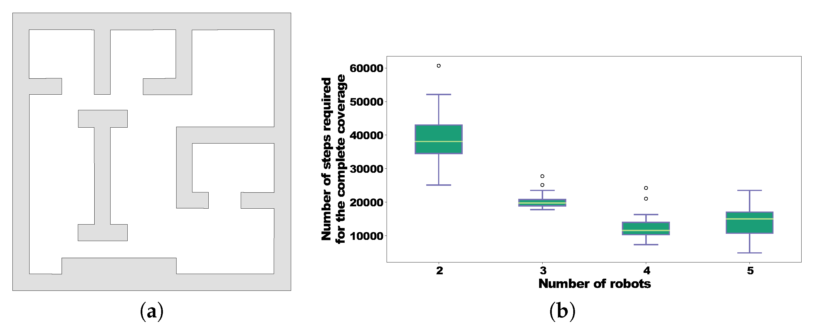
5.1. Results of a Joint Trajectory of Multiple Robots for Coverage

We implemented our multi-robot coverage Algorithm 1 in the simulation. We used a laboratory environment shown in Figure 6a and the associated configuration space $X_{\mathrm{free}}$ in the environment for a disk robot such as iRobot Create 2.0 or Roomba. The iRobot Create 2.0 has various sensors, but we utilized only the contact sensors and the clock. Then, we verified our Algorithm 1 on $X_{\mathrm{free}}$ using a set of bouncing angles $\Phi =\left\{{135}^{\circ }\right\}$ for two robots, where both used the same bouncing angle and speed, and had identical sensing. For all the experiments and simulation runs of this article, we considered 8 different robot orientations of $S^1$ with ${45}^{\circ }$ separation between each orientation. The smaller blue and green circles of Figure 6b represent the initial locations of the two robots in their configuration space, and colored arrowheads starting from the circles (→ for the green robot and ← for the blue robot) represent their orientations. The bigger blue and green circles of Figure 6c also represent the two robots’ initial locations in their workspace. A joint trajectory starting from the initial configuration or locations generated from the simulation that covers the environment is depicted by blue and green arrows in Figure 6b and blue and green lines in Figure 6c as paths of blue and green robots. To validate the simulated joint trajectory using a physical experiment, we used two iRobot Create 2.0 robots and two Arduino Uno microcontrollers to drive them. There is also an identical C++ program running on Arduinos that allows the robots to move forward in the free space at a fixed speed and rotate ${135}^{\circ }$ after bumping at the boundary of the environment or with each other. Figure 6d–f show three different snapshots of the physical experiment. The video of the experiment can be found at https://youtu.be/zcSXAVGFVqE.

In addition, we validated our Algorithm 1 for two simulation environments of Figure 7a and Figure 8a considering multiple robots and the same bouncing angle $\varphi ={135}^{\circ }$ for all of them. The first environment is a $10\times 10$ grid containing obstacles in it and the second environment is a $15\times 15$ grid having obstacles inside of it. We used different numbers of robots (e.g., $m=2,3,4,5$) and random initial configurations for all robots in various simulation runs. We ran 20 simulation tests for both environments and demonstrated the plots in Figure 7b and Figure 8b, comparing the result of the number of steps required for the complete coverage of the environments and the number of robots used. These plots imply that the number of steps required for covering the entire environment decreases with the increase in the number of robots. In an environment with more obstacles, the increase in the number of robots does not guarantee the less number of steps required for the coverage of the entire environment due to the robot-robot collisions and the intricacy of the environment itself. An example of that is illustrated in Figure 8b, where the number of steps required for the complete coverage of the given environment with 5 robots is larger than the number of steps required for the complete coverage of the same environment with 4 robots. Furthermore, we tested our Algorithm 1 for covering a larger simulation environment of Figure 9a utilizing a random initial configuration for $m=10$ robots and their same bouncing angle $\varphi ={135}^{\circ }$. This environment is a $20\times 12$ grid with more obstacles. The heatmap of an almost complete (98%) environment coverage provided by the joint trajectory of 10 robots is shown in Figure 9b. This result demonstrates that our multi-robot coverage approach works significantly well even for larger environments despite the limited use of sensors in robots.

5.2. Results of Persistent Monitoring of Target Regions

We also implemented our Algorithm 2 in the simulation for multi-robot persistent monitoring of target regions in the environment. We validated our algorithm with a simulation environment and a set of bouncing angles $\Phi =\left\{{45}^{\circ }\right\}$. We found $r=47$ periodic groups that represent the overlapping trajectories of two robots for two target regions covered by their paths in the environment, as illustrated in Figure 10. Therefore, these trajectories monitor the target regions persistently avoiding collisions with one another. In Figure 10a, the initial locations of the two robots are delineated with smaller blue and green circles and their orientations are delineated with colored arrowheads (→) starting from the circles. In Figure 10b, their initial locations are also delineated with blue and green circles. The overlapping trajectories of blue and green robots starting from their initial configuration in the configuration space are shown with blue and green arrows respectively in Figure 10a. The same overlapping trajectories starting from their initial locations in the workspace are shown with blue and green lines in Figure 10b.

Again, we computed the free configuration space of the environment $X_{\mathrm{free}}$ of the iRobot Create robot for a second indoor environment (illustrated in Figure 11a). Then, we tested our algorithm on $X_{\mathrm{free}}$ for monitoring a subset of target regions of the environment utilizing a set of bouncing angles $\Phi =\left\{{90}^{\circ }\right\}$ for two robots, where both of them again used the same bouncing angle and speed, and had identical sensing. We found $r=18$ periodic groups that represent the overlapping trajectories of the two robots to monitor the target regions in the environment covered by their paths (as illustrated in Figure 11b in the configuration space and in Figure 11c) in the workspace) persistently avoiding collisions with one another. Similarly, the smaller blue and green circles of Figure 11b represent the initial locations of the two robots in their configuration space, and colored arrowheads starting from the circles (→ for the blue robot and ↓ for the green robot) represent their orientations. The bigger blue and green circles of Figure 11c also represent the two robots’ initial locations in their workspace. The overlapping trajectories of blue and green robots starting from their initial configuration in the configuration space are illustrated with blue and green arrows respectively in Figure 11b. The same overlapping trajectories of blue and green robots starting from their initial locations in the workspace are illustrated with blue and green lines respectively in Figure 11c.

We implemented the overlapping trajectories of the two robots in a distributed manner in a physical experiment using two iRobot Create 2.0 robots and two Arduino Unos. As mentioned before, the iRobot Create utilizes only the contact sensors and the clock. A similar C++ program runs on both Arduinos that makes the robots move forward in the free space at a fixed speed and rotate ${90}^{\circ }$ after bumping at the boundary of the environment. Figure 11d–f also show three different snapshots of the physical experiment for overlapping and collision-free trajectories of the two robots. The experiment video can be found at https://youtu.be/v3bSkt9Wvas.

6. Conclusions and Future Work

We have addressed the problem of coverage of the given environment and persistent monitoring of some target regions in the environment by a number of bouncing robots. In our proposed approach, we constructed a joint trajectory for multiple bouncing robots incrementally until they covered the environment completely. We found some periodic cycle based collision-free and overlapping trajectories of multiple robots to monitor the target regions for a long period of time. Finally, we presented simulation results and physical experiments to validate the performance of our approach.

We chose ${45}^{\circ }$, ${90}^{\circ }$, and ${135}^{\circ }$ as bouncing angles in our experiments due to the ease of implementation in physical robot platforms. We found that ${135}^{\circ }$ and ${45}^{\circ }$ angles provide better coverage since they sample more orientation angles (8) as opposed to ${90}^{\circ }$(4) and ${180}^{\circ }$ (2) angles. We utilized 8 orientation angles as the discretization resolution of $S^1$ in our experiments and simulation runs. On the other hand, the discretization of free space E is related to the size of the workspace and the number of robots. In terms of computational complexity, our cell-to-cell mapping is linear in the number of cells in the discretized configuration space. For Algorithm 1, the computation time depends on the number of cells in the generated joint trajectory. For Algorithm 2, since coordination is required, the computation time depends on the total number of cells in the entire free configuration space $X_{\mathrm{free}}$.

In the future, we plan to extend our approach to solving the offline coverage and exploration problems using multiple bouncing robots. We can also develop a method to apply the modified cell-to-cell mapping in a subspace of the high dimensional configuration space of multiple robots to reduce the computational time. It will be a more practical approach to incorporate a bounded uncertainty for both rotation and translation of the robots which will lead to the development of a probabilistic variant of our method in a future effort of this research. In this context, we can build on our previous work [9], where we considered uncertainty in rotation for a single robot for solving the coverage problem or use results from a recent work [14] that have characterized nondeterministic uncertainty for a single bouncing robot.

Moreover, one immediate extension of our ideas is augmenting the range of applications. First, our simple bouncing strategy can work in aquatic robots such as Unmanned Surface Vehicles (USVs), Autonomous Underwater Vehicles (AUVs), and so on. Generating coverage and persistent monitoring paths for AUVs is particularly useful since these environments are naturally GPS-denied. Second, bouncing events do not necessarily have to be against physical boundaries. Bouncing can be performed on detecting certain events and landmarks, which can be treated as virtual obstacles [8]. We would also like to extend our persistent monitoring approach in a privacy-preserving scenario, where robots are not allowed to use cameras and other security-threatening sensors.

References

1. Alam, T.; Reis, G.M.; Bobadilla, L.; Smith, R.N. A Data-Driven Deployment Approach for Persistent Monitoring in Aquatic Environments. In Proceedings of the IEEE International Conference on Robotic Computing (IRC), Laguna Hills, CA, USA, 31 January–2 February 2018; pp. 147–154. [Google Scholar]
2. Mulgaonkar, Y.; Makineni, A.; Guerrero-Bonilla, L.; Kumar, V. Robust aerial robot swarms without collision avoidance. IEEE Robot. Autom. Lett. 2017, 3, 596–603. [Google Scholar] [CrossRef]
3. Nilles, A.Q.; Pervan, A.; Berrueta, T.A.; Murphey, T.D.; LaValle, S.M. Information Requirements of Collision-Based Micromanipulation. In Proceedings of the Workshop on the Algorithmic Foundations of Robotics (WAFR), Oulu, Finland, 21–23 June 2020. [Google Scholar]
4. O’Kane, J.M.; LaValle, S.M. Localization with limited sensing. IEEE Trans. Robot. 2007, 23, 704–716. [Google Scholar] [CrossRef]
5. Alam, T.; Bobadilla, L.; Shell, D.A. Space-efficient filters for mobile robot localization from discrete limit cycles. IEEE Robot. Autom. Lett. 2018, 3, 257–264. [Google Scholar] [CrossRef]
6. Stavrou, D.; Panayiotou, C. Localization of a simple robot with low computational-power using a single short range sensor. In Proceedings of the IEEE International Conference on Robotics and Biomimetics (ROBIO), Guangzhou, China, 11–14 December 2012; pp. 729–734. [Google Scholar]
7. Erickson, L.H.; Knuth, J.; O’Kane, J.M.; LaValle, S.M. Probabilistic localization with a blind robot. In Proceedings of the IEEE International Conference on Robotics and Automation (ICRA), Pasadena, CA, USA, 19–23 May 2008; pp. 1821–1827. [Google Scholar]
8. Bobadilla, L.; Martinez, F.; Gobst, E.; Gossman, K.; LaValle, S.M. Controlling wild mobile robots using virtual gates and discrete transitions. In Proceedings of the American Control Conference (ACC), Montreal, QC, Canada, 27–29 June 2012; pp. 743–749. [Google Scholar]
9. Alam, T.; Bobadilla, L.; Shell, D.A. Minimalist robot navigation and coverage using a dynamical system approach. In Proceedings of the IEEE International Conference on Robotic Computing (IRC), Taichung, Taiwan, 10–12 April 2017; pp. 249–256. [Google Scholar]
10. Lewis, J.S.; O’Kane, J.M. Guaranteed navigation with an unreliable blind robot. In Proceedings of the IEEE International Conference on Robotics and Automation (ICRA), Anchorage, AK, USA, 3–7 May 2010; pp. 5519–5524. [Google Scholar]
11. Mastrogiovanni, F.; Sgorbissa, A.; Zaccaria, R. Robust navigation in an unknown environment with minimal sensing and representation. IEEE Trans. Syst. Man Cybern. 2009, 39, 212–229. [Google Scholar] [CrossRef] [PubMed]
12. Tovar, B.; Guilamo, L.; LaValle, S.M. Gap navigation trees: Minimal representation for visibility-based tasks. In Proceedings of the Workshop on the Algorithmic Foundations of Robotics (WAFR), Zeist, The Netherlands, 11–13 July 2004; pp. 425–440. [Google Scholar]
13. Nilles, A.Q.; Becerra, I.; LaValle, S.M. Periodic trajectories of mobile robots. In Proceedings of the IEEE/RSJ International Conference on Intelligent Robots and Systems (IROS), Vancouver, BC, Canada, 24–28 September 2017; pp. 3020–3026. [Google Scholar]
14. Nilles, A.Q.; Ren, Y.; Becerra, I.; LaValle, S.M. A visibility-based approach to computing nondeterministic bouncing strategies. In Proceedings of the Workshop on the Algorithmic Foundations of Robotics (WAFR), Merida, Mexico, 9–11 December 2018; pp. 89–104. [Google Scholar]
15. Choset, H. Coverage for robotics–A survey of recent results. Ann. Math. Artif. Intell. 2001, 31, 113–126. [Google Scholar] [CrossRef]
16. Karapetyan, N.; Benson, K.; McKinney, C.; Taslakian, P.; Rekleitis, I. Efficient multi-robot coverage of a known environment. In Proceedings of the IEEE/RSJ International Conference on Intelligent Robots and Systems (IROS), Vancouver, BC, Canada, 24–28 September 2017; pp. 1846–1852. [Google Scholar]
17. Choset, H.; Pignon, P. Coverage path planning: The boustrophedon cellular decomposition. In Field and Service Robotics; Springer: London, UK, 1998; pp. 203–209. [Google Scholar]
18. Soltero, D.E.; Smith, S.L.; Rus, D. Collision avoidance for persistent monitoring in multi-robot systems with intersecting trajectories. In Proceedings of the IEEE/RSJ International Conference on Intelligent Robots and Systems (IROS), San Francisco, CA, USA, 25–30 September 2011; pp. 3645–3652. [Google Scholar]
19. Hsu, C.S. A theory of cell-to-cell mapping dynamical systems. J. Appl. Mech. 1980, 47, 931–939. [Google Scholar] [CrossRef]
20. Hsu, C.S. Cell-To-Cell Mapping: A Method of Global Analysis for Nonlinear Systems; Springer Science & Business Media: Berlin/Heidelberg, Germany, 2013; Volume 64. [Google Scholar]
21. Burridge, R.R.; Rizzi, A.A.; Koditschek, D.E. Sequential composition of dynamically dexterous robot behaviors. Int. J. Robot. Res. 1999, 18, 534–555. [Google Scholar] [CrossRef]
22. Alam, T. A Dynamical System Approach for Resource-Constrained Mobile Robotics. Ph.D. Thesis, Florida International University, Miami, FL, USA, 2018. [Google Scholar]
23. Galceran, E.; Carreras, M. A survey on coverage path planning for robotics. Robot. Auton. Syst. 2013, 61, 1258–1276. [Google Scholar] [CrossRef] [Green Version]
24. Volos, C.K.; Kyprianidis, I.M.; Stouboulos, I.N. Experimental investigation on coverage performance of a chaotic autonomous mobile robot. Robot. Auton. Syst. 2013, 61, 1314–1322. [Google Scholar] [CrossRef]
25. Gabriely, Y.; Rimon, E. Spanning-tree based coverage of continuous areas by a mobile robot. Ann. Math. Artif. Intell. 2001, 31, 77–98. [Google Scholar] [CrossRef]
26. Agmon, N.; Hazon, N.; Kaminka, G.A. The giving tree: Constructing trees for efficient offline and online multi-robot coverage. Ann. Math. Artif. Intell. 2008, 52, 143–168. [Google Scholar] [CrossRef]
27. Hazon, N.; Kaminka, G.A. On redundancy, efficiency, and robustness in coverage for multiple robots. Robot. Auton. Syst. 2008, 56, 1102–1114. [Google Scholar] [CrossRef]
28. Zheng, X.; Jain, S.; Koenig, S.; Kempe, D. Multi-robot forest coverage. In Proceedings of the IEEE/RSJ International Conference on Intelligent Robots and Systems (IROS), Edmonton, AB, Canada, 2–6 August 2005; pp. 3852–3857. [Google Scholar]
29. Fazli, P.; Davoodi, A.; Pasquier, P.; Mackworth, A.K. Complete and robust cooperative robot area coverage with limited range. In Proceedings of the IEEE/RSJ International Conference on Intelligent Robots and Systems (IROS), Taipei, Taiwan, 18–22 October 2010; pp. 5577–5582. [Google Scholar]
30. Fazli, P.; Davoodi, A.; Mackworth, A.K. Multi-robot repeated area coverage. Auton. Robots 2013, 34, 251–276. [Google Scholar] [CrossRef] [Green Version]
31. Fazli, P.; Mackworth, A.K. The effects of communication and visual range on multi-robot repeated boundary coverage. In Proceedings of the IEEE International Symposium on Safety, Security, and Rescue Robotics (SSRR), College Station, TX, USA, 5–8 November 2012; pp. 1–8. [Google Scholar]
32. Smith, S.L.; Rus, D. Multi-robot monitoring in dynamic environments with guaranteed currency of observations. In Proceedings of the IEEE Conference on Decision and Control (CDC), Atlanta, GA, USA, 15–17 December 2010; pp. 514–521. [Google Scholar]
33. Smith, S.L.; Schwager, M.; Rus, D. Persistent robotic tasks: Monitoring and sweeping in changing environments. IEEE Trans. Robot. 2012, 28, 410–426. [Google Scholar] [CrossRef] [Green Version]
34. Lan, X.; Schwager, M. Planning periodic persistent monitoring trajectories for sensing robots in gaussian random fields. In Proceedings of the IEEE International Conference on Robotics and Automation (ICRA), Karlsruhe, Germany, 6–10 May 2013; pp. 2415–2420. [Google Scholar]
35. Yu, J.; Schwager, M.; Rus, D. Correlated orienteering problem and its application to persistent monitoring tasks. IEEE Trans. Robot. 2016, 32, 1106–1118. [Google Scholar] [CrossRef]
36. Akella, S.; Hutchinson, S. Coordinating the motions of multiple robots with specified trajectories. In Proceedings of the IEEE International Conference on Robotics and Automation (ICRA), Washington, DC, USA, 11–15 May 2002; pp. 624–631. [Google Scholar]
37. Snape, J.; Van Den Berg, J.; Guy, S.J.; Manocha, D. Independent navigation of multiple mobile robots with hybrid reciprocal velocity obstacles. In Proceedings of the IEEE/RSJ International Conference on Intelligent Robots and Systems (IROS), St. Louis, MO, USA, 10–15 October 2009; pp. 5917–5922. [Google Scholar]
38. Cassandras, C.G.; Lin, X.; Ding, X. An optimal control approach to the multi-agent persistent monitoring problem. IEEE Trans. Autom. Control 2013, 58, 947–961. [Google Scholar] [CrossRef]
39. LaValle, S.M. Planning Algorithms; Cambridge University Press: Cambridge, UK, 2006; Available online: http://lavalle.pl/planning/ (accessed on 1 June 2020).
40. Van Der Spek, J.A.W. Cell Mapping Methods: Modifications and Extensions. Ph.D. Thesis, Eindhoven University of Technology, Eindhoven, The Netherlands, 1994. [Google Scholar]
Figure 1. An example scenario. An indoor environment, with multiple robots moving through the space.
Robotics 09 00047 g001
Figure 2. Simple bouncing strategy. (a) A robot rotates counterclockwise by the bouncing angle ϕ with respect to its current direction while it bounces off of the boundary of the environment. (b) When two robots collide with each other (only in the multi-robot coverage task), they then turn counterclockwise with their bouncing angles ϕ 1 , ϕ 2 from their current moving orientations.
Robotics 09 00047 g002
Figure 3. Trajectory generation and neighbor selection. (a) A generated trajectory x ˜ from an initial configuration x 0 . (b) The best nearest neighbor β l (green square) among unprocessed neighbors of last cell b of the trajectory x ˜ .
Robotics 09 00047 g003
Figure 4. A joint trajectory of the robots connecting through the new neighboring cell β l .
Robotics 09 00047 g004
Figure 5. Two cycle forming scenarios. (a) The same initial and ending cell b. (b) Different initial and ending cells.
Robotics 09 00047 g005
Figure 6. From the simulation to the physical implementation. (a) An artificial lab environment to cover. (bc) A joint trajectory of the two robots in their configuration space and workspace respectively, generated from our simulation using the set of bouncing angles Φ = { 135 } . The initial configuration of the two robots is depicted in (b) by blue and green circles for their locations and by colored arrowheads starting from these circles for their orientations. Their initial locations are also depicted in (c) by blue and green circles. There is only one robot-robot collision in the middle of the upper part of the environment. (df) Three different snapshots at different times of the physical experiment of the generated joint trajectory of two iRobot Create 2.0 robots controlled with two Arduinos.
Robotics 09 00047 g006
Figure 7. Simulation results of the multi-robot coverage. (a) The first simulation environment. (b) The comparison result of the number of steps required for the complete coverage of the first environment and the number of robots used.
Robotics 09 00047 g007
Figure 8. Simulation results of the multi-robot coverage. (a) The second simulation environment. (b) The comparison result of the number of steps required for the complete coverage of the second environment and the number of robots used.
Robotics 09 00047 g008
Figure 9. Simulation result of the multi-robot coverage for a larger simulation environment. (a) A random initial configuration of 10 robots in the environment representing their locations with the centers of the circles and orientations with colored arrowheads inside circles. (b) An environment coverage heatmap provided by the joint trajectory of 10 robots starting from their initial configuration.
Robotics 09 00047 g009
Figure 10. Simulation result. Overlapping and collision-free trajectories of the two robots in their configuration space in (a) and workspace in (b) respectively that monitor two regions in the given environment persistently starting from the encircled locations and using the set of bouncing angles Φ = { 45 } .
Robotics 09 00047 g010
Figure 11. From the simulation to the physical implementation. (a) Another artificial lab environment. (b,c) Overlapping and collision-free trajectories of the two robots in their configuration space and workspace respectively, found from our simulation that monitor two regions in the given environment persistently starting from the encircled locations and using the set of bouncing angles Φ = { 90 } . (df) Three different snapshots at different times of a distributed physical implementation of overlapping and collision-free trajectories of two iRobot Create 2.0 robots controlled with two Arduinos.
Robotics 09 00047 g011aRobotics 09 00047 g011b