Rapid Evaluation and Validation Method of Above Ground Forest Biomass Estimation Using Optical Remote Sensing in Tundi Reserved Forest Area, India


Abstract
1. Introduction
2. Materials and Methods
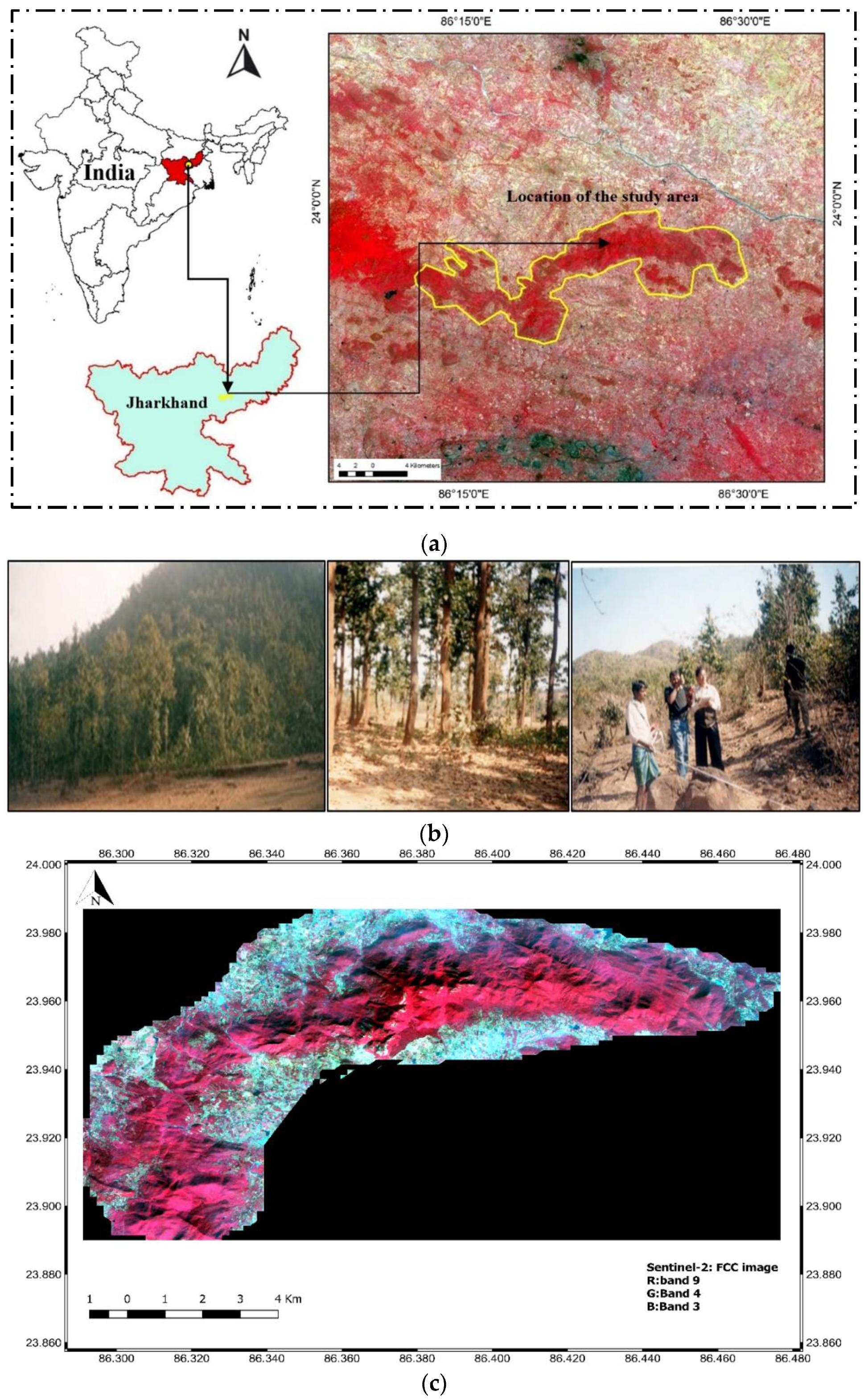
2.1. Study Area
2.2. Datasets
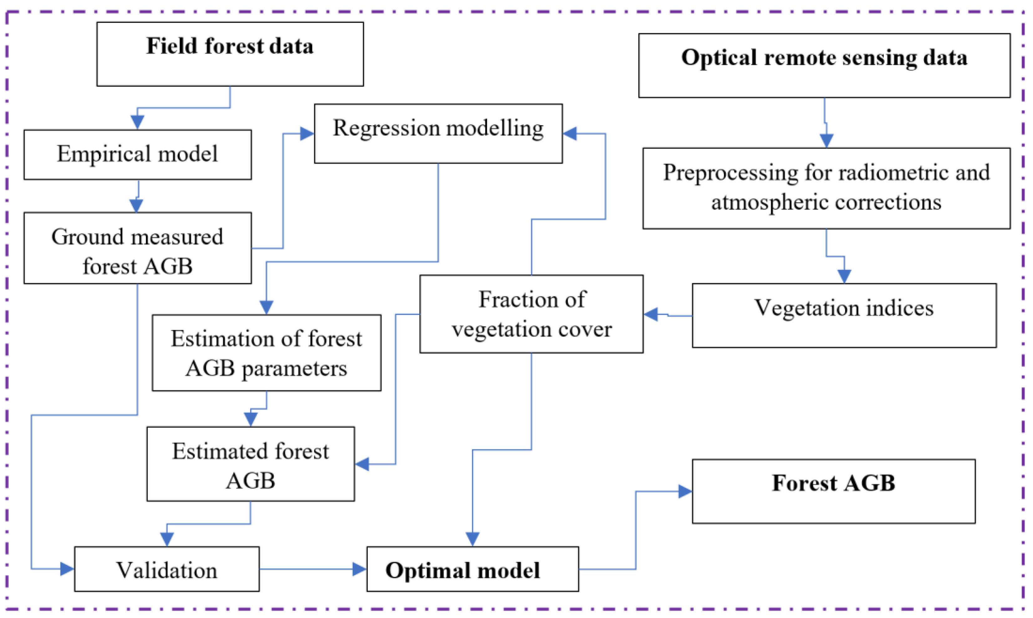
2.3. Methodology
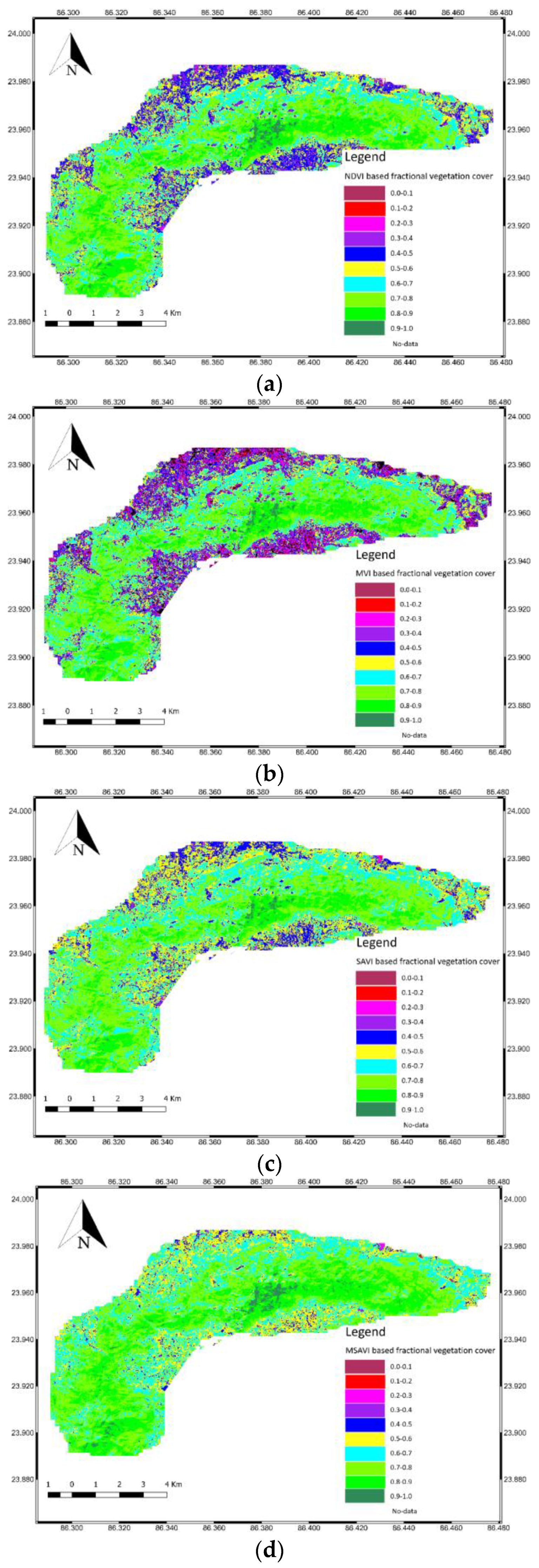
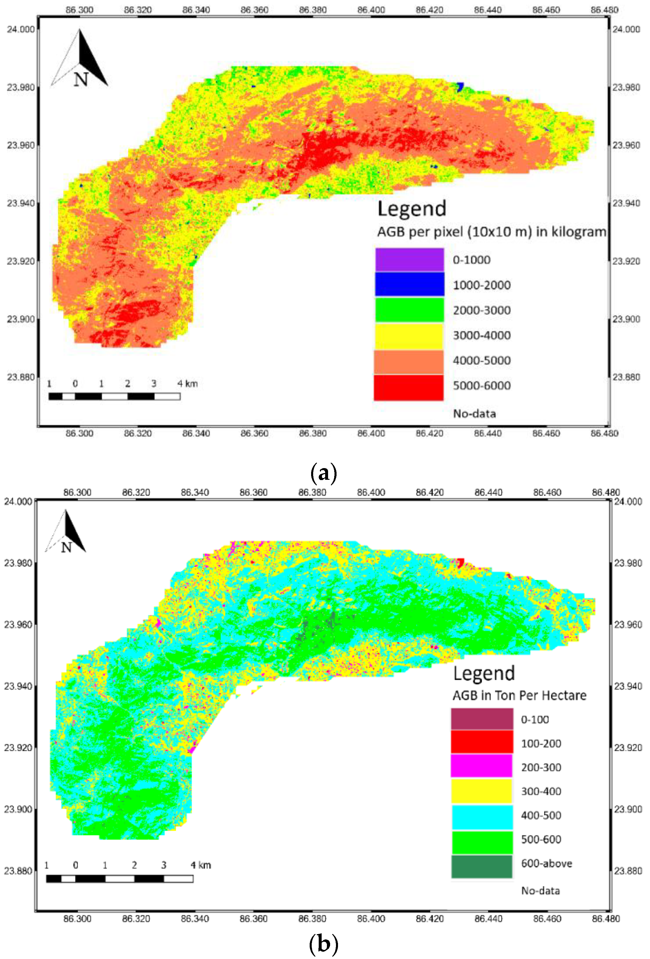
3. Results and Discussion
4. Conclusions
Author Contributions
Funding
Institutional Review Board Statement
Informed Consent Statement
Data Availability Statement
Acknowledgments
Conflicts of Interest
References
- Norovsuren, B.; Tseveen, B.; Batomunkuev, V.; Renchin, T. Estimation for forest biomass and coverage using Satellite data in small scale area, Mongolia. In IOP Conference Series: Earth and Environmental Science; IOP Publishing: Beijing, China, 2019; Volume 320, p. 012019. [Google Scholar]
- Kumar, P.; Krishna, A.P.; Nathawat, M.S.; Singh, C.P.; Mohan, S. Tree height estimation in Tundi Reserved Forest using SAR Interferometry. In Proceedings of the Microwave Remote Sensing of the Atmosphere and Environment V, Goa, India, 7 December 2006; Volume 6410, p. 641004-1. [Google Scholar]
- Köhl, M.; Lasco, R.D.; Cifuentes, M.; Jonsson, Ö.; Korhonen, K.; Mundhenk, P.; Návar, J.; Stinson, G. Changes in forest production, biomass and carbon: Results from the 2015 UN FAO Global Forest Resource Assessment. For. Ecol. Manag. 2015, 352, 21–34. [Google Scholar]
- Tian, X.; Yan, M.; van der Tol, C.; Li, Z.; Su, Z.; Chen, E.; Li, X.; Li, L.; Wang, X.; Pan, X.; et al. Modeling forest above-ground biomass dynamics using multi-source data and incorporated models: A case study over the qilian mountains. Agric. For. Meteorol. 2017, 246, 1–14. [Google Scholar] [CrossRef]
- Asner, G.P.; Mascaro, J.; Muller-Landau, H.C.; Vieilledent, G.; Vaudry, R.; Rasamoelina, M.; Hall, J.S.; Van Breugel, M. A universal airborne LiDAR approach for tropical forest carbon mapping. Oecologia 2011, 168, 1147–1160. [Google Scholar] [CrossRef] [PubMed]
- Johnson, D.J.; Needham, J.; Xu, C.; Massoud, E.C.; Davies, S.J.; Anderson-Teixeira, K.J.; Bunyavejchewin, S.; Chambers, J.Q.; Chang-Yang, C.; Chiang, J.; et al. Climate sensitive size-dependent survival in tropical trees. Nat. Ecol. Evolut. 2018, 2, 1436–1442. [Google Scholar] [CrossRef] [PubMed]
- Kumar, A.; Saikia, P.; Saikia, P.; Deka, J.; Bharali, S.; Singha, L.; Tripathi, O.; Khan, M.L. Tree diversity assessment and above ground forests biomass estimation using SAR remote sensing: A case study of higher altitude vegetation of North-East Himalayas, India. Phys. Chem. Earth Parts A/B/C 2019, 111, 53–64. [Google Scholar] [CrossRef]
- Champion, S.H.; Seth, S.K. A Revised Survey of the Forest Types of India; Amazon.com, Inc.: Delhi, India, 1968. [Google Scholar]
- Pandit, S.; Tsuyuki, S.; Dube, T. Estimating Above-Ground Biomass in Sub-Tropical Buffer Zone Community Forests, Nepal, Using Sentinel 2 Data. Remote. Sens. 2018, 10, 601. [Google Scholar] [CrossRef]
- Komolafe, E.T.; Chukwuka, K.S.; Obiakara, M.C.; Osonubi, O. Carbon stock and sequestration potential of Ibodi monkey forest in Atakumosa, Osun state, Nigeria. Trees For. People 2020, 2, 100031. [Google Scholar] [CrossRef]
- Laurin, G.V.; Balling, J.; Corona, P.; Mattioli, W.; Papale, D.; Puletti, N.; Rizzo, M.; Truckenbrodt, J.; Urban, M. Above-ground biomass prediction by Sentinel-1 multitemporal data in central Italy with integration of ALOS2 and Sentinel-2 data. J. Appl. Remote Sens. 2018, 12, 016008. [Google Scholar] [CrossRef]
- Lefsky, M.A. A global forest canopy height map from the Moderate Resolution Imaging Spectroradiometer and the Geoscience Laser Altimeter System. Geophys. Res. Lett. 2010, 37, L15401. [Google Scholar] [CrossRef]
- Liu, Z.; Liu, P.W.; Massoud, E.; Farr, T.G.; Lundgren, P.; Famiglietti, J.S. Monitoring Groundwater Change in California′s Central Valley Using Sentinel-1 and GRACE Observations. Geosciences 2019, 9, 436. [Google Scholar] [CrossRef]
- Massoud, E.C.; Xu, C.; Fisher, R.A.; Knox, R.G.; Walker, A.P.; Serbin, S.P.; Christoffersen, B.O.; Holm, J.A.; Kueppers, L.M.; Ricciuto, D.M.; et al. Identification of key parameters controlling demographically structured vegetation dynamics in a land surface model: CLM4. 5 (FATES). Geosci. Model Dev. 2019, 12, 4133–4164. [Google Scholar] [CrossRef]
- Running, S.W.; Nemani, R.; Heinsch, F.A.; Zhao, M.; Reeves, M.; Hashimoto, H. A Continuous Satellite-Derived Measure of Global Terrestrial Primary Production. Bioscience 2004, 54, 547–560. [Google Scholar] [CrossRef]
- Arun, D.; Kulkarni, B.L. Random Forest Algorithm for Land Cover Classification. Int. J. Recent Innov. Trends Comput. Commun. 2016, 4, 58–63. [Google Scholar]
- Galidaki, G.; Zianis, D.; Gitas, I.; Radoglou, K.; Karathanassi, V.; Tsakiri–Strati, M.; Woodhouse, G.; Mallinis, G. Vegetation biomass estimation with remote sensing: Focus on forest and other wooded land over the Mediterranean ecosystem. Int. J. Remote Sens. 2017, 38, 1940–1966. [Google Scholar] [CrossRef]
- Çolak, E.; Sunar, A.F. Remote sensing & GIS integration for monitoring the areas affected by forest fires: A case study in Izmir, Turkey. Int. Arch. Photogramm. Remote Sens. Spat. Inf. Sci. 2018, 42, 165–170. [Google Scholar]
- Borrás, J.; Delegido, J.; Pezzola, A.; Pereira, M.; Morassi, G.; Camps-Valls, G. Land use classification from Sentinel-2 imagery. Rev. Teledetección 2017, 48, 55–66. [Google Scholar]
- Immitzer, M.; Vuolo, F.; Einzmann, K.; Ng, W.T.; Böck, S.; Atzberger, C. Suitability of Sentinel-2 Data for Tree Species Classification in Central Europe. WorldView 2013, 2, 16. [Google Scholar]
- Tsolmon, R.; Tateishi, R.; Tetuko, J.S.S. A method to estimate forest biomass and its application to monitor Mongolian Taiga using JERS-1 SAR data. Int. J. Remote Sens. 2002, 23, 4971–4978. [Google Scholar] [CrossRef]
- Chen, L.; Ren, C.; Zhang, B.; Wang, Z.; Xi, Y. Estimation of forest above-ground biomass by geographically weighted regression and machine learning with Sentinel imagery. Forests 2018, 9, 582. [Google Scholar] [CrossRef]
- Kumar, P.; Krishna, A.P. InSAR based Tree Height Estimation of Hilly Forest using Multi-Temporal Radarsat-1 and Sentinel-1 SAR data. IEEE J. Sel. Top. Appl. Earth Obs. Remote Sens. 2019, 12, 5147–5152. [Google Scholar] [CrossRef]
- Puletti, N.; Chianucci, F.; Castaldi, C. Use of Sentinel-2 for forest classification in Mediterranean environments. Ann. Silvic. Res. 2017, 42, 32–38. [Google Scholar]
- Zhang, Y.; Liang, S.; Yang, L. A Review of Regional and Global Gridded Forest Biomass Datasets. Remote Sens. 2019, 11, 2744. [Google Scholar] [CrossRef]
- Li, Y.; Wang, H.; Li, X.B. Fractional vegetation cover estimation based on an improved selective endmember spectral mixture model. PLoS ONE 2015, 10, e0124608. [Google Scholar] [CrossRef]
- Chave, J.; Andalo, C.; Brown, S.; Cairns, M.A.; Chambers, J.Q.; Eamus, D.; Lescure, J.P. Tree allometry and improved estimation of carbon stocks and balance in tropical forests. Oecologia 2005, 145, 87–99. [Google Scholar] [CrossRef] [PubMed]
- Lim, K.; Treitz, P.; Wulder, M.; St-Onge, B.; Flood, M. LiDAR remote sensing of forest structure. Prog. Phys. Geogr. Earth Environ. 2003, 27, 88–106. [Google Scholar] [CrossRef]
- Palace, M.W.; Sullivan, F.B.; Ducey, M.J.; Treuhaft, R.N.; Herrick, C.; Shimbo, J.Z.; Mota-E-Silva, J. Estimating forest structure in a tropical forest using field measurements, a synthetic model and discrete return lidar data. Remote Sens. Environ. 2015, 161, 1–11. [Google Scholar] [CrossRef]
- Saatchi, S.; Harris, N.L.; Brown, S.; Lefsky, A.M.; Mitchard, E.T.A.; Salas, W.; Zutta, B.R.; Buermann, W.; Lewis, S.L.; Hagen, S.; et al. Benchmark map of forest carbon stocks in tropical regions across three continents. Proc. Natl. Acad. Sci. USA 2011, 108, 9899–9904. [Google Scholar] [CrossRef] [PubMed]
- Wu, X.; Wang, X.; Wu, Y.; Xia, X.; Fang, J. Forest biomass is strongly shaped by forest height across boreal to tropical forests in China. J. Plant Ecol. 2015, 8, 559–567. [Google Scholar] [CrossRef]
- Solberg, S.; Naesset, E.; Gobakken, T.; Bollandsås, O.M. Forest biomass change estimated from height change in interferometric SAR height models. Carbon Balance Manag. 2014, 9, 5. [Google Scholar] [CrossRef]
- Yu, Y.; Saatchi, S.; Heath, L.S.; LaPoint, E.; Myneni, R.; Knyazikhin, Y. Regional distribution of forest height and biomass from multisensor data fusion. J. Geophys. Res. Biogeosci. 2010, 115, 16. [Google Scholar] [CrossRef]
- Zhang, G.; Ganguly, S.; Nemani, R.R.; White, M.A.; Milesi, C.; Hashimoto, H.; Wang, W.; Saatchi, S.; Yu, Y.; Myneni, R.B. Estimation of forest aboveground biomass in California using canopy height and leaf area index estimated from satellite data. Remote Sens. Environ. 2014, 151, 44–56. [Google Scholar] [CrossRef]
- Zhang, X.; Kondragunta, S. Estimating forest biomass in the USA using generalized allometric models and MODIS land products. Geophys. Res. Lett. 2006, 33, 09402. [Google Scholar] [CrossRef]
- Berner, L.T.; Law, B.E. Plant traits, productivity, biomass, and soil properties from forest sites in the Pacific Northwest, 1999–2014. Sci. Data 2016, 3, 160002. [Google Scholar] [CrossRef] [PubMed]
- Chen, J.M. Evaluation of Vegetation Indices and a Modified Simple Ratio for Boreal Applications. Can. J. Remote Sens. 1996, 22, 229–242. [Google Scholar] [CrossRef]
- Durante, P.; Martín-Alcón, S.; Gil-Tena, A.; Algeet, N.; Tomé, J.L.; Recuero, L.; Palacios-Orueta, A.; Oyonarte, C. Improving Aboveground Forest Biomass Maps: From High-Resolution to National Scale. Remote Sens. 2019, 11, 795. [Google Scholar] [CrossRef]
- Hansen, M.C.; Potapov, P.V.; Moore, R.; Hancher, M.; Turubanova, S.A.; Tyukavina, A.; Thau, D.; Stehman, S.V.; Goetz, S.J.; Loveland, T.R.; et al. High-Resolution Global Maps of 21st-Century Forest Cover Change. Science 2013, 342, 850–853. [Google Scholar] [CrossRef] [PubMed]
- Asner, G.P.; Hughes, R.F.; Varga, T.A.; Knapp, D.E.; Kennedy-Bowdoin, T. Environmental and Biotic Controls over Aboveground Biomass throughout a Tropical Rain Forest. Ecosystems 2009, 12, 261–278. [Google Scholar] [CrossRef]
- Frolking, S.; Palace, M.W.; Clark, D.B.; Chambers, J.Q.; Shugart, H.H.; Hurtt, G.C. Forest disturbance and recovery: A general review in the context of spaceborne remote sensing of impacts on aboveground biomass and canopy structure. J. Geophys. Res. Biogeosci. 2009, 114, G00E02. [Google Scholar] [CrossRef]
- McEwan, R.W.; Lin, Y.-C.; Sun, I.F.; Hsieh, C.-F.; Su, S.-H.; Chang, L.-W.; Song, G.-Z.M.; Wang, H.-H.; Hwong, J.-L.; Lin, K.-C.; et al. Topographic and biotic regulation of aboveground carbon storage in subtropical broad-leaved forests of Taiwan. For. Ecol. Manag. 2011, 262, 1817–1825. [Google Scholar] [CrossRef]
- Ministry of Environment Forest and Climate Change. State of Forest Report; Forest Survey of India (Ministry of Environment Forest and Climate Change, GoI): Uttarakhand, India, 2019; Volume 1, pp. 66–85.
- Rawat, J.K.; Singh, S.; Mishra, R. Santhal Pargana Forest Report; Government of Jharkhand: Ranchi, India, 2010; pp. 15–87.
- Astola, H.; Häme, T.; Sirro, L.; Molinier, M.; Kilpi, J. Comparison of Sentinel-2 and Landsat 8 imagery for forest variable prediction in boreal region. Remote. Sens. Environ. 2019, 223, 257–273. [Google Scholar] [CrossRef]
- Zhang, S.; Chen, H.; Fu, Y.; Niu, H.; Yang, Y.; Zhang, B. Fractional vegetation cover estimation of different vegetation types in the Qaidam Basin. Sustainability 2019, 11, 864. [Google Scholar] [CrossRef]
- Qazi, W.A.; Baig, S.; Gilani, H.; Waqar, M.M.; Dhakal, A.; Ammar, A. Comparison of forest aboveground biomass estimates from passive and active remote sensing sensors over Kayar Khola watershed, Chitwan district, Nepal. J. Appl. Remote. Sens. 2017, 11, 26038. [Google Scholar] [CrossRef]


| Subsystem | Band Number | Wavelength Range (μm) | Band Central Wavelength (μm) | Bandwidth (nm) | Spatial Resolution (m) |
|---|---|---|---|---|---|
| VNIR | 1 | 0.43–0.45 | 0.443 (Coastal aerosol) | 20 | 60 |
| 2 | 0.46–0.52 | 0.490 (BLUE) | 65 | 10 | |
| 3 | 0.54–0.58 | 0.560 (GREEN) | 35 | ||
| 4 | 0.65–0.68 | 0.665 (RED) | 30 | ||
| 5 | 0.70–0.71 | 0.705 (Vegetation RED edge) | 15 | 20 | |
| 6 | 0.73–0.75 | 0.749 (Vegetation RED edge) | 15 | ||
| 7 | 0.77–0.79 | 0.783 (Vegetation RED edge) | 20 | ||
| 8 | 0.78–0.90 | 0.842 (NIR) | 115 | 10 | |
| 8a | 0.86–0.88 | 0.865 (Vegetation RED edge) | 20 | 20 | |
| 9 | 0.93–0.95 | 0.945 (Water vapor) | 20 | 60 | |
| 10 | 1.37–1.39 | 1.375 (SWIR—Cirrus) | 30 | ||
| SWIR | 11 | 1.57–1.66 | 1.610 (SWIR) | 90 | 20 |
| 12 | 2.10–2.28 | 2.190 (SWIR) | 180 |
| Sample Location Number | Easting | Northing | Number of Trees | Average Tree Height (m) | Average DBH (cm) (at 4.5 ft Above Ground) |
|---|---|---|---|---|---|
| SL1 | 23°57′53.10″ | 86°28′23.80″ | 17 | 10.9 | 71.01 |
| SL2 | 23°58′06.38″ | 86°23′08.47″ | 19 | 23.33 | 142.49 |
| SL3 | 23°54′49.91″ | 86°19′30.53″ | 24 | 15.8 | 80.57 |
| SL4 | 23°57′58.28″ | 86°24′18.87″ | 23 | 19.7 | 91.64 |
| SL5 | 23°57′21.22″ | 86°22′35.17″ | 22 | 17.8 | 104.33 |
| SL6 | 23°57′40.13″ | 86°23′06.37″ | 20 | 19.84 | 95.18 |
| SL7 | 23°57′05.10″ | 86°22′26.32″ | 16 | 15.55 | 104.23 |
| SL8 | 23°53′59.99″ | 86°18′55.75″ | 15 | 17.4 | 97.02 |
| SL9 | 23°56′51.50″ | 86°22′22.10″ | 16 | 12.6 | 92.76 |
| SL10 | 23°54′53.80″ | 86°19′35.49″ | 22 | 12.86 | 87.76 |
| SL11 | 23°58′26.81″ | 86°25′03.14″ | 15 | 9.65 | 82.56 |
| SL12 | 23°58′27.79″ | 86°26′25.76″ | 17 | 10.5 | 77.59 |
| SL13 | 23°54′51.86″ | 86°17′49.35″ | 21 | 9.8 | 73.48 |
| SL14 | 23°58′04.77″ | 86°27′31.11″ | 18 | 13.4 | 75.88 |
| SL15 | 23°58′19.68″ | 86°25′56.25″ | 19 | 12.8 | 75.34 |
| SL16 | 23°57′39.16″ | 86°22′51.61″ | 18 | 13.6 | 78.12 |
| SL17 | 23°57′02.19″ | 86°19′53.71″ | 22 | 14.35 | 77.62 |
| SL18 | 23°58′04.77″ | 86°23′01.88″ | 27 | 8.75 | 67.34 |
| SL19 | 23°57′37.53″ | 86°27′11.29″ | 24 | 10.8 | 68.41 |
| SL20 | 23°56′41.77″ | 86°20′56.10″ | 18 | 13.6 | 77.78 |
| SL21 | 23°57′34.62″ | 86°20′45.56″ | 16 | 11.9 | 71.27 |
| SL22 | 23°58′18.06″ | 86°23′36.30″ | 25 | 11.85 | 66.6 |
| Sample Location Number | FVC (GROUND) | FVC (NDVI) | FVC (MVI) | FVC (SAVI) | FVC (MSAVI) |
|---|---|---|---|---|---|
| SL1 | 0.29 | 0.58 | 0.56 | 0.57 | 0.26 |
| SL2 | 0.99 | 0.98 | 0.97 | 0.97 | 0.77 |
| SL3 | 0.67 | 0.78 | 0.77 | 0.77 | 0.54 |
| SL4 | 0.91 | 0.90 | 0.90 | 0.89 | 0.71 |
| SL5 | 0.90 | 0.93 | 0.92 | 0.92 | 0.71 |
| SL6 | 0.84 | 0.90 | 0.90 | 0.89 | 0.66 |
| SL7 | 0.57 | 0.80 | 0.80 | 0.78 | 0.47 |
| SL8 | 0.56 | 0.78 | 0.77 | 0.77 | 0.46 |
| SL9 | 0.41 | 0.71 | 0.70 | 0.70 | 0.35 |
| SL10 | 0.55 | 0.70 | 0.68 | 0.69 | 0.44 |
| SL11 | 0.26 | 0.59 | 0.56 | 0.57 | 0.24 |
| SL12 | 0.31 | 0.59 | 0.57 | 0.58 | 0.27 |
| SL13 | 0.33 | 0.61 | 0.57 | 0.58 | 0.29 |
| SL14 | 0.40 | 0.62 | 0.60 | 0.61 | 0.34 |
| SL15 | 0.41 | 0.63 | 0.60 | 0.61 | 0.34 |
| SL16 | 0.42 | 0.67 | 0.64 | 0.64 | 0.35 |
| SL17 | 0.54 | 0.70 | 0.67 | 0.68 | 0.44 |
| SL18 | 0.35 | 0.55 | 0.50 | 0.53 | 0.29 |
| SL19 | 0.39 | 0.60 | 0.56 | 0.58 | 0.33 |
| SL20 | 0.42 | 0.64 | 0.62 | 0.63 | 0.35 |
| SL21 | 0.30 | 0.59 | 0.56 | 0.57 | 0.26 |
| SL22 | 0.44 | 0.63 | 0.59 | 0.61 | 0.36 |
| Vegetation Indices | NDVI | MVI | SAVI | MSAVI |
|---|---|---|---|---|
| R | 0.9696 | 0.9599 | 0.9677 | 0.9981 |
| MAE | 0.1941 | 0.1729 | 0.1793 | 0.0947 |
| Sample Location Number | AGB (kg) (Ground) | FVC (MSAVI) |
|---|---|---|
| SL1 | 18659.89 | 0.26 |
| SL2 | 160815.21 | 0.77 |
| SL3 | 34821.50 | 0.54 |
| SL4 | 56166.84 | 0.71 |
| SL5 | 65778.21 | 0.70 |
| SL6 | 61020.63 | 0.66 |
| SL7 | 57353.44 | 0.47 |
| SL8 | 55605.20 | 0.46 |
| SL9 | 36807.44 | 0.35 |
| SL10 | 33626.20 | 0.44 |
| SL11 | 22331.11 | 0.24 |
| SL12 | 21460.73 | 0.27 |
| SL13 | 17964.20 | 0.29 |
| SL14 | 26194.07 | 0.34 |
| SL15 | 24666.35 | 0.34 |
| SL16 | 28177.79 | 0.35 |
| SL17 | 29352.34 | 0.44 |
| SL18 | 13470.94 | 0.29 |
| SL19 | 17159.58 | 0.33 |
| SL20 | 27933.05 | 0.35 |
| SL21 | 20521.26 | 0.26 |
| SL22 | 17844.75 | 0.36 |
| Sample Location Number | Ground AGB (in kg) | Image AGB (Proposed) | Image AGB (Qazi et al. Model) | Image AGB (Pandit et al. Model) |
|---|---|---|---|---|
| SL1 | 18659.89 | 18840.10 | 17989.54 | 18469.38 |
| SL17 | 29352.34 | 30196.83 | 34432.89 | 32746.29 |
| SL18 | 13470.94 | 14310.09 | 13934.32 | 15583.64 |
| SL19 | 17159.58 | 17551.79 | 16930.83 | 17184.53 |
| SL20 | 27933.05 | 28272.18 | 31030.86 | 30734.47 |
| SL21 | 20521.26 | 19412.03 | 24418.61 | 21435.69 |
| SL22 | 17844.75 | 18221.16 | 20692.22 | 18974.25 |
Publisher’s Note: MDPI stays neutral with regard to jurisdictional claims in published maps and institutional affiliations. |
© 2021 by the authors. Licensee MDPI, Basel, Switzerland. This article is an open access article distributed under the terms and conditions of the Creative Commons Attribution (CC BY) license (http://creativecommons.org/licenses/by/4.0/).
Share and Cite
Kumar, P.; Krishna, A.P.; Rasmussen, T.M.; Pal, M.K. Rapid Evaluation and Validation Method of Above Ground Forest Biomass Estimation Using Optical Remote Sensing in Tundi Reserved Forest Area, India. ISPRS Int. J. Geo-Inf. 2021, 10, 29. https://doi.org/10.3390/ijgi10010029
Kumar P, Krishna AP, Rasmussen TM, Pal MK. Rapid Evaluation and Validation Method of Above Ground Forest Biomass Estimation Using Optical Remote Sensing in Tundi Reserved Forest Area, India. ISPRS International Journal of Geo-Information. 2021; 10(1):29. https://doi.org/10.3390/ijgi10010029
Chicago/Turabian StyleKumar, Praveen, Akhouri P. Krishna, Thorkild M. Rasmussen, and Mahendra K. Pal. 2021. "Rapid Evaluation and Validation Method of Above Ground Forest Biomass Estimation Using Optical Remote Sensing in Tundi Reserved Forest Area, India" ISPRS International Journal of Geo-Information 10, no. 1: 29. https://doi.org/10.3390/ijgi10010029
APA StyleKumar, P., Krishna, A. P., Rasmussen, T. M., & Pal, M. K. (2021). Rapid Evaluation and Validation Method of Above Ground Forest Biomass Estimation Using Optical Remote Sensing in Tundi Reserved Forest Area, India. ISPRS International Journal of Geo-Information, 10(1), 29. https://doi.org/10.3390/ijgi10010029