Article

Estimating the Soil Erosion Cover-Management Factor at the European Part of Russia

Institute of Environmental Sciences, Kazan Federal University, 420008 Kazan, Russia
*
Author to whom correspondence should be addressed.
ISPRS Int. J. Geo-Inf. 2021, 10(10), 645; https://doi.org/10.3390/ijgi10100645
Submission received: 23 July 2021 / Revised: 17 September 2021 / Accepted: 22 September 2021 / Published: 25 September 2021
(This article belongs to the Special Issue Earth Observation and GIScience for Agricultural Applications)

Abstract

:
Evaluation of the vegetation and agricultural-management factor (C-factor) is an important task, the solution of which affects the correct assessment of the intensity of soil erosion. For the vast area of the European part of Russia (EPR), this task is particularly relevant since no products allow taking into account the C-factor. An approach based on automated interpretation of the main crop groups based on MODIS satellite imaging data from Terra and Aqua satellites with the LSTM machine-learning method was used to achieve this goal. The accuracy of crop group recognition compared to the open data of the Federal State Statistics Service of Russia was 94%. The resulting crop maps were used to calculate the C-factor for each month of a particular year from 2014 to 2019. After that, summaries were made at the regional and landscape levels. The average C-factor value for the EPR was 0.401, for the forest landscape zone 0.262, for the forest-steppe zone 0.362, and for the steppe zone 0.454. The obtained results are in good correlation with the results of previous field studies and provide up-to-date (based on 2014–2019 data) estimates of C-factor for rainfall erosion (monthly, annual) with high spatial detail (250 m).

1. Introduction

In recent decades, due to the changes in the climate in the study area, the contribution of snowmelt runoff to soil erosion has significantly decreased. Therefore, an important task is the assessment of the soil losses due to rainfall runoff [1]. The vegetation and agricultural-management factor (C-factor) is a key parameter in soil erosion models. The methods of vegetation factor (C-factor) estimation used in the erosion equations have been considered in many Russian and foreign publications concerning soil erosion models. A complete review of existing methods for assessing vegetation cover and management factors for various erosion models was carried out in the works of G.A. Larionov [2], L.F. Litvin [3], F.N. Lisetsky et al. [4], monographs “Catchment erosion-fluvial systems” ed. R.S. Chalov et al. [5] and the article by Q. Feng et al. [6]. In addition to the USLE [7] and RUSLE [8], the C-factor is also applied in other erosion models, such as ANSWERS (Areal Nonpoint SourceWatershed Environment Response Simulation) [9], SWAT (Soil and Water Assessment Tool) [10], and SEMMED (Soil Erosion Model for Mediterranean Regions) [11]. Soil erosion assessments are conducted at various scales. They may cover particular slopes [12], small [13] and large watersheds [14], regions [15], countries, and continents [16,17]. C-factor estimation methods that are appropriate for one scale are usually not appropriate for other scales.
Two standard empirical methods exist to obtain C-factor values in the USLE/RUSLE models. The first one–the C-factor, is defined as the soil loss ratio from the land under specified vegetation cover to the corresponding loss from clean-tilled, continuous fallow. The second one-the C-factor, is calculated as a product of five sub-factors described in the RUSLE handbook [8]. Researchers in different countries have adopted the calculation methods to local conditions, but the method, in general, has not changed. The US Soil Conservation Service uses the values of agricultural management factors, summarized within particular regions of the United States [4]. A quantitative assessment of the soil-protective properties of crops for the USLE equation for the territory of the USSR was carried out at Moscow State University [18]. In the absence of a sufficient number of unified measurements of soil washout, the soil-protective properties of crops were determined using a projective coverage monthly for the forest and steppe zones [18,19]. In the work of Morgun et al. [20], the values and dynamics of C- factor (calculated based on generalized field data of various authors) for the main crops (winter, spring, maize and sunflower, beets and potatoes, perennial herbs) for the forest-steppe zone of Ukraine are presented. The monograph “Catchment erosion-fluvial systems” [5] contains particular erosion indices of crops combined into four groups:
  • Thick cover (winter and spring crops, leguminous crops, annual grasses)
  • Tilled high-stem (corn, sunflower)
  • Tilled low-stem (potatoes, sugar beet)
  • Perennial grasses (second-third years of vegetation)
The data are presented for six periods of the year’s warm season, determined by the main stages of cultivation and phases of crop vegetation.
Annual soil loss by erosion was determined for the European territory of Russia. In these estimations, very generalized regional values of soil-protective properties of vegetation were taken into account. The average soil erosion in the study area amounts to 4.04 t ha−1 year−1, considering the soil-protective coefficients of crops [21].
Estimation of the C-factor using empirical methods based on field experiments is very laborious and expensive to perform. Therefore, alternative methods to assess the C-factor at the regional and national levels are used. Currently, there are three main groups of such methods.
(1) C-factor values from literature or field data are assigned to corresponding vegetation types [13,22,23,24,25,26,27,28,29]. The enhanced method is used on the territory of the European Union, where European land cover databases (for example, CORINE Land Cover), biophysical parameters obtained by remote sensing data, and statistical data on crops and practices are used as source data. The C-factor was estimated using crop statistics (% of land per crop) and data on management practices such as conservation tillage, plant residues, and winter crop cover in arable lands. The C-factor in non-arable lands was estimated using the vegetation cover dataset FCover [16,17]. In some works, the vegetation factor’s lack of a seasonal component is noted as a disadvantage of this approach. Even in Europe in neighbor countries, the seasons with the most intense rainfall belong to different periods of the year, when soil vegetation (especially crops) is completely different [30].
(2) Calculation of linear and non-linear regressions between the values of vegetation indices and the values of C-factor obtained in the field to consider spatial and seasonal variability [31,32,33,34,35,36]. The most commonly used index is NDVI (Normalized Difference Vegetation Index) and EVI (Enhanced Vegetation Index). The main problems associated with NDVI are soil reflectance (especially in the case of sparse vegetation) and the variability of vegetation period. Several soil-adjusted indices, such as TSAVI (Transformed Soil-Adjusted Vegetation Index) [37] and PVI (Perpendicular Vegetation Index) [38], have been developed to consider soil reflectance. The main effects of vegetation phases occur during earlier growth stages when the NDVI often overestimates thin vegetation cover due to intense chlorophyll activity and vegetation senescence when vegetation indices typically decrease even when the cover remains the same [39]. Along with this, many studies using vegetation indices analyze the seasonal effect when estimating C- factor, including both monthly and annual periods [40,41,42].
(3) Calculation of regressions between C-factor and projective coverage. Projective coverage, usually used in such models, cannot reflect contributions from different vegetation layers to soil conservation. The effects of vegetation structures on soil erosion control are ignored. For example, the mixed forest is more effective than pure forest at reducing soil erosion, although both types of forests exhibit the same level of cover. The leaf area index (LAI) has been used as a vegetation structure index to replace projective coverage [6].
In general, none of the methods discussed above is ideal because they do not allow to carry out a comprehensive assessment of the effect of vegetation on reducing erosion. There are two main directions of research in this area: maximum consideration of all the soil-protective properties of vegetation, including biophysical properties, projective coverage, vegetation structure, seasonal vegetation features, etc., and extrapolation of values over large areas, taking into account spatial variability. So, there is no unified methodology for assessing this factor, and this topic is still actual and open to discussion. Also, the relevance is largely determined by the variety of landscape conditions and features of land-use systems in different countries.
For the first time for this vast region of the Earth, the results of estimating the vegetation factor for calculating soil erosion are presented. They are relevant both in time, spatial detail, and used methods, in contrast to previous small-scale assessments provided on the study area. The huge area of Russia and the inaccessibility of many regions for field research makes it necessary to use remote sensing data. In addition, the assessment for such large areas was previously carried out only for the European Union territory [16]. Using the actual climatic data, Copernicus FCover data (vegetation projective cover), and VNP22Q2 data from the VIIRS satellite (data allow determining the beginning and end of the growing season), the phenological phases of vegetation and the seasonality of precipitation were taken into account. This allowed to obtain not fixed values of the C-factor for specific types of vegetation, but also to obtain monthly estimates taking into account the latitudinal landscape zoning. Thus, the proposed study contributes to solving the problem of assessing C-factor for the eastern part of Europe. Also, it should be noted that the study is largely methodological in fact.
The main aim of this study is to assess C-factor for the European Russia territory. To achieve this aim, several tasks were solved:
  • The seasonality of precipitation has been determined, i.e., areas with rainfalls in a particular month are identified;
  • Due to the lack of government statistical and spatial data on the structure of cultivated areas and crop rotation, crop recognition was carried out using data from peer territories (Canada);
  • Using free products of biophysical parameters calculated on the basis of remote sensing data, the phenological phases of vegetation were determined;
  • The annual and monthly mean values of C-factor for the study area were calculated.

2. Materials and Methods

2.1. Study Area

The European part of Russia (EPR) covers approximately 4 million km2 and is situated over several landscape zones, from tundra to temperate zone deserts. According to the Land Cover Map obtained in 2014 from satellite data from TerraNorte RLC v.3 [43], which was designed by the Space Research Institute of the Russian Academy of Science (RAS), the total area of arable lands in the EPR comprises approximately 600,000 km2. Approximately 95 million people live in this region, which is the majority of Russia’s population. The environmental conditions that accompany soil erosion in this vast territory are diverse. We created and published a dedicated online geoportal called ‘The River Basins of the European Territory of Russia’ (http://bassepr.kpfu.ru/ accessed on 15 September 2021) that displays the environmental conditions of the territory (terrain, climate, hydrology, soils, land use, human-induced impact) [44].

2.2. Input Data

The assessment of the C-factor for the territory of European Russia was carried out using data from remote sensing of the Earth from space. The extensive spatial coverage caused the choice of the source data. The spatial and temporal resolution of the data was considered. We used products obtained from satellite data and available on the USGS/NASA (USA) and Copernicus websites (a joint program of the European Commission and the European Space Agency):
  • Products MOD13Q1, MYD13Q1 obtained from the MODIS satellite imagery data from Terra and Aqua satellites-16-day composites of NDVI and EVI vegetation indices with a spatial resolution of 250 m;
  • VNP22Q2 products obtained from VIIRS satellite imagery data from the Suomi NPP satellite-annual indicators of the phenology of the land surface with a spatial resolution of 500 m. The product contains six phenological transition dates: onset of greenness increase, the onset of greenness maximum, the onset of greenness decrease, the onset of greenness minimum, dates of mid-green, and senescence phases;
  • FCover product obtained from PROBA-V satellite imagery data. 10-day composites of the biophysical parameter FCover-the fraction of the surface covered by any green vegetation type, with a spatial resolution of 300 m.
The Russian product was also used-the annual map of terrestrial ecosystems of Russia TerraNorte RLC created by the Space Research Institute of the Russian Academy of Sciences [43,45] based on MODIS satellite data. It represents the spatial distribution of the main types of land cover with a spatial resolution of 230 m.
The total volume of satellite data obtained from open archives is about 370 GB.

2.3. C-Factor Assessment Method

The contemporary assessment of the soil-protective role of vegetation (including agrocenoses) was performed based on the above mentioned RS data for the 2014–2019 observation period. The value of the C-factor in rainfall runoff was assessed. The general scheme of the process of C factor assessment is shown in Figure 1.
The C-factor was estimated monthly for “warm” months. “Warm months” -are months when liquid forms of precipitation fall. For such a large area as the EPR, “warm” months were determined in each pixel. In order to do this the average monthly temperatures at 204 meteorological stations of EPR were calculated based on daily air temperature observations at Roshydromet. Spatial interpolation was done for the entire study region using the Multilevel B-spline Approximation method [46], and “indicator” rasters were built for each month, I(i), i = 1,...,12, where 1 or 0 in pixel indicated i-th month as “warm” or “cold”, respectively (Figure 2).
Assessment of soil-protective properties of vegetation in the i-th month of the j-th year was carried out separately (by different methods) on arable lands and on all other types of lands (non-arable).

2.3.1. C-Factor Assessment on Arable Land

Arable land (pixels) was identified using the TerraNorte RLC annual map. In each pixel, the C-factor changes from month to month depending on the agrotechnical management and growing season phases of crops. It also changes from year to year due to crop rotation and differences in soil-protective properties of crops. The C(i,j) (C-factor in the i-th month of the j-th year) on arable land were calculated.
The developed approach to assess C(i,j) on arable land consisted in the recognition of crops by multi-temporal remote sensing data of the j-th year and the assessment of the C-factor in the i-th month of this year, and taking into account phenological metrics, FCover, and values of soil protection coefficients of crops in 6 periods of the warm part of the year.
For automated crops recognition, MODIS composites (MOD13Q1, MYD13Q1) were used, including time series of NDVI and EVI for the growing season of each year. Data in the peer territories were used as training samples.
As peer territories, several Canadian regions that are located in the temperate climate zone of humid plains and their landscape and climatic conditions are close to the conditions of the ETR were considered. For these territories, data from the Annual Crop Inventory project of the Ministry of Agriculture and Food of Canada for 2011–2018 are publicly available [47]. These are land use/land cover rasters with a spatial resolution of 30 m, including the classification of various crops.
The list of recognizable crops and groups of crops included crops represented both in the territories of analogs and in the studied territory-legumes, corn, spring cereals, winter cereals, sunflower, sugar beet, potatoes, buckwheat, fallow lands, perennial grasses, as well as nurseries and gardens. Pixels of MODIS data, covered more than 80% by one crop according to the Annual Crop Inventory data were chosen for training. The created training samples are subsets of MODIS rasters on the territory of Canada for the vegetative seasons of 2015–2017. They contain the values of NDVI, EVI, and the QA (quality assesment) layer in sample pixels with a temporal step of 8 days. A total of 30 NDVI, EVI, and QA rasters were used for each year. The index value was considered acceptable if the pixel value on the reliability raster equaled 0 (“Good data”) or 1 (“Marginal data”). The preprocessing included filling missing data using Cubic Spline interpolation (in individual pixels for particular dates), plotting, generalizing, analyzing graphs of the seasonal variation of indices for various crops, and studying their variability, etc. The NDVI and EVI series of the current year (30-dimensional vectors in each pixel) were used as input data to the recognition algorithm for training and classification.
On the stage of development of the automated recognition technique, numerous experiments were carried out to test different classification methods: feedforward neural networks with deep learning (Deep Learning MultiLayer Perceptron, MLP) [48], Random Forest (RF) [49], recurrent neural networks (Long short-term memory, LSTM) [50]. The learning and classification algorithms that implement these methods were developed in Python 3.7 using the Keras v.2.3.1 + Tensorflow v.2.2.0 framework, with a GPU (computation on a video card). For data preprocessing, post-processing, and analysis, codes in R v.3.4.4 were developed. During the tests, the accuracy of recognition was assessed by different methods (producers’s accuracy, user accuracy, commission and omission errors), including cross-validation. MLP method showed the worst results; The RF method recognized well the widely represented in the territories classes of crops (the per cent of correctly recognized pixels was about 90%). Still, it poorly recognized the underrepresented crops, despite attempts to balance the sample. The LSTM method showed the best recognition quality (percent of correct recognition 94%). Its advantage can be explained by the fact that it’s aimed at recognizing sequences, which is important in our case. Table 1 shows the recognition accuracy of the classes of crops by the above methods using the data in the analogous territories.
The trained recognition algorithm using the LSTM method was applied for arable land in the European Russia territory for 2014–2019. The input data to the algorithm was a set of NDVI, EVI rasters, and MODIS quality layers for the study area for the vegetative season of each year. The result was six raster layers, where codes of crops (or groups of crops) in a particular year were assigned in the pixels of the arable land.
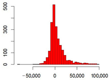
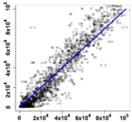
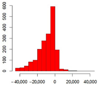
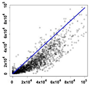
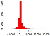
At the next stage, the quality of crop recognition was assessed. For this aim, we used open data from the Federal State Statistics Service (Rosstat), namely the Database of indicators of municipalities (https://rosstat.gov.ru/dbscripts/munst/ accessed on 15 September 2021). Information about the sown areas of crops in the municipal districts of the European part of Russia was obtained by queries to this Database. This data was geocoded using the vector layer of the district’s boundaries. Next, for the 1120 districts where arable land is present, the areas covered by a particular crop were estimated according to the recognition results, after which a comparison with Rosstat data for 2014–2019. The Table 2 shows the generalized results of comparisons by groups of main crops presented in government statistics.
As we can observe, the correlation between the obtained results and the Rosstat data is quite high. Mean values and medians of area differences are about zero. The frequency histograms of the difference values demonstrate the degree of underestimation or overestimation of certain categories of crops in more detail. The recognition quality was assessed as quite acceptable for our purposes.
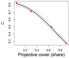
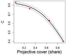
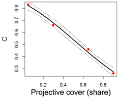
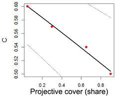
The next stage consisted of converting the raster of crops recognized for the j-th year to the values of the C-factor in the i-th month of this year in pixels of arable land. For this, the following procedure was performed. The basis was the soil protection coefficients (erosion indices) of crops for six periods of the warm part of the year determined using literature [5,16,17] (Table 3). It was decided to realize the “pessimistic” scenario. Because there is no information about the yield and agricultural techniques, the values of the erosion indices of crops were assigned in the suggestion of using moldboard ploughing. Also, using the sigmoid function a/(1 + exp ((b-X)/c)), a mathematical approximation of the dependence of the erosion indices on the projective cover was performed for four periods of the warm part of the year-from the beginning of the growing season to harvesting. The results are shown in the Table 3 (values of the sigmoid parameters) and, in more detail, in the Table 4.
For the j-th year, in each pixel of arable land, according to the phenological metrics of the VNP22Q2 product, the dates of the beginning and end of the vegetation season were determined. They were taken as the beginning of the 2nd and the end of the 5th periods, respectively. For the i-th “warm” month, the fractions (per cent of days) of three-time intervals were calculated in the pixel: (1) before the beginning of the vegetation season, (2) during the vegetation season, and (3) after its end. For example, in a pixel in the territory of the Republic of Tatarstan for January, the first fraction is 100%, the second and third-0%, and for May, the first fraction can be 20%, the second 80%, the third 0%. In the range from the beginning of the vegetation season to harvesting (periods 2–5), the FCover data was used as a parameter of the projective cover (step of 10 days). FCover values on these days of the month were recalculated into C values using a sigmoid, the parameters of which depended on the crop type in the pixel. Then average C values were calculated. It was more difficult to calculate C in the 1st and 6th periods due to the lack of complete information on the timing of the main tillage. In the “pessimistic” scenario, we chose the main tillage option for all crops shortly after harvest. So, the 6th period (stubble) was ignored (the properties of the 1st period were assigned).
Further, the C-factor in the i-th “warm” month in the pixel was estimated as a weighted average of the obtained C values in three ranges of the month: (1) for days before the start of the growing season, (2) for days during the vegetation season and (3) for days after its end. The weights are the fraction of the corresponding ranges in the i-th month. A slightly different approach has been taken for perennial grasses where there is no such problem. Here, the assessment was carried out in the same way as for meadow vegetation of non-arable lands.

2.3.2. C-Factor Assessment on Non-Arable Land

To estimate C(i,j) (C-factor in the i-th month of the j-th year) on non-arable lands, the approach described in work by Panagos et al. [43] was applied. Following the most cited literature data, ranges of C-factor values were assigned for the land cover classes of non-arable lands in the annual map of TerraNorte RLC (Table 5).
Urban areas, wetlands, water bodies, permanent snow and ice, bare lands, and rocks were not included in the assessment. The effect of vegetation density was quantified using the FCover biophysical parameter, normalized in the 0–1 range. In each pixel of non-arable land, the C-factor in the i-th “warm” month of the j-th year was estimated as (1):
C(i,j) = Cmax + (Cmin − Cmax)·FCover(i,j),
where FCover(i,j) is the FCover value averaged over all days of the i-th month of the j-th year; Cmin, Cmax—minimum and maximum values of the C-factor for the land cover class in a pixel (Table 5). C-factor reaches its maximum value when FCover is 0 and minimum value when FCover is 1.
At the final step, the rasters C(i,j) of arable land and C(i,j) of non-arable land were combined into single rasters (mosaics) C(i,j), representing the spatial distribution of the C-factor for the “warm” months of 2014–2019 in the European territory of Russia.

3. Results and Discussion

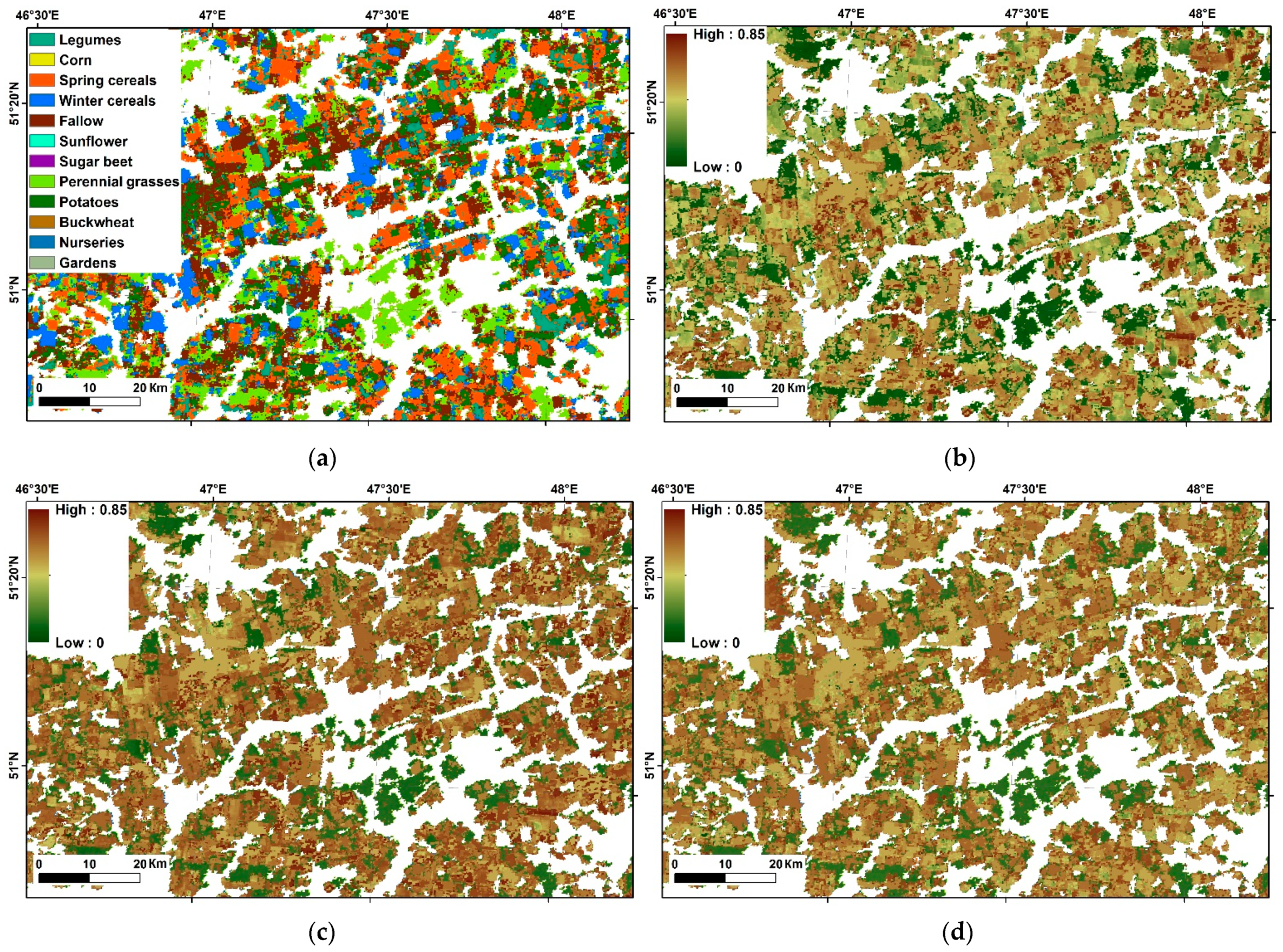
According to the developed approach, the C-factor was calculated for the agrocenoses of European Russia for each “warm” month of 2014–2019. The Figure 3 shows fragments of the results for June, August, and October 2016.
Using the obtained estimates of C(i,j) for arable and non-arable lands, various generalizations were made. Raster layers representing the spatial distribution of generalized estimates were calculated:
(1) C-factor of the j-th year (warm period) - annual estimates of the C-factor for rainfall runoff for 2014–2019. The values were averaged in the “warm” months in a pixel, taking into account the erosion potential of rainfall (fractions of the annual) (2):
C(j) = (R(1,j)·C(1,j)·I(1) + R(2,j)·C(2,j)·I(2) + … + R(12,j) ·C(12,j) ·I(12))/R(j),
where I(i)—indicator function “warm”/“cold” in the i-th month, and R(1,j) ∙ I(i)-erosion potential of precipitation in the i-th month of the j-th year;
(2) C-factor in the i-th month, the long-term average (3):
Ccp(i) = (C(i,2014) ·I(i) + … + C(i,2019) ·I(i))/N,
where N = 6 years;
(3) C-factor average long-term annual (in a warm period, with rainfall) (4):
Cmean = (C2014 + … + C2019)/N,
where N = 6 years.
The Figure 4 shows thematic maps of the average long-term C-factor for each month (on a small scale) and the long-term annual C-factor for the study area. In Figure 5 individual fragments of these maps are shown in more detail.
For the territory of European Russia, the obtained values of the average long-term annual C-factor vary in the range from 0.0006 to 0.808, the mean value is 0.1264, and the standard deviation is 0.1796. For agrocenoses, these values are 0.0199, 0.808, 0.401, 0.1686, respectively. The results obtained earlier for the European Union [16]: mean C-factor 0.1043, standard deviation 0.1046, range 0.0001 to 0.526. At the same time, on arable land, the mean is 0.233, and without considering soil protection management 0.287.
To assess the reliability of the results, their agreement with the results of the 2010 studies [5] was checked. The data on the soil-protective capacity of agrocenoses (erosion indices), weighted over crop areas and generalized for the main natural agricultural zones, are presented here. In addition, the results were compared with the data obtained for the landscape zones of European Russia in the studies of 2012–2014 [51]. These data are obtained from field observations. The Table 6 presented C-factor values on the agrocenoses of European Russia in previous studies and the results of our study.
We can see that for the entire European part of Russia, the average value of the annual C-factor is absolutely the same. For landscape zones, the difference in the values of the C-factor on agrocenoses compared with the 2010 data ranges from −10% to 20%, and with 2012–2014 from −5 to 15%. Such values demonstrate a high degree of agreement, which indicates the adequacy of our approach and the reliability of the obtained results. It makes no sense to discuss the difference or dynamics of the C-factor estimates considering the difference in the used methods and their accuracy.
Thus, for the European part of Russia, as a result of the study, modern (2014–2019) estimates of the C-factor for rain erosion (monthly, annual) with high spatial detail (250 m) were obtained.

4. Conclusions

Approaches to studying the dependence of the C-factor from the vegetation indices obtained from the remote sensing data and modeling such dependencies are widely used now [32,36,52,53,54]. But in most cases, such models are obtained for small regions and, if applied without calibration for other territories, they give wrong results. The developed method uses climatic, biophysical, and phenological parameters. It allowed obtaining adequate results for such a large study area, considering latitudinal zonality.
The developed model needs to consider all the features of crop rotations on arable land, land cultivation methods, etc. However, the methodology provides results for different scenarios by adjusting the values and the timing of the main tillage in pixels of arable land. The most feasible is correcting the C-factor values based on crop rotations according to the data of long-term recognition of crop types. As a rule, for agricultural land specializing in cereals and leguminous crops, 5–6 field crop rotations are used. Therefore, accounting for these crop rotations types is a solvable task. However, the problem is assessing land plowing methods, which is the most significant adjusting to the C-factor value. To consider the plowing techniques, analyzing the historical methods of tillage in a particular area or recommended plowing for a particular crop could be carried out.
The model gives results that are most similar to the data obtained from field observations of previous years. We should note that the results were obtained in one scenario. The most reliable results can be obtained considering data about the structure of sown areas and the methods of soil cultivation, which, unfortunately, are currently unavailable in Russia. As noted earlier, it is possible to take into account these parameters using indirect data. This approach will be tested in further studies.
Nevertheless, we can say that the data obtained as a result of the study already take into account the maximum possible set of open resources currently available for the territory of Russia. The obtained data could significantly improve the assessment and modelling of modern erosion-accumulative processes. The developed methodology makes it possible to assess the C-factor in the European territory of Russia. The results also have practical importance. Now, within the framework of the project, they are used to calculate soil erosion losses in the study area, along with estimates of the factors R, K, etc. In the future, the applicability of the developed methodology to the eastern part of Russia will be assessed, which has regional conditions that differ from the European part and analogous territories.

Author Contributions

Conceptualization, Oleg Yermolaev and Svetlana Mukharamova; methodology, Svetlana Mukharamova, Anatoly Saveliev, Artur Gafurov and Maxim Ivanov; software, Svetlana Mukharamova and Anatoly Saveliev, validation, Svetlana Mukharamova, Artur Gafurov, Anatoly Saveliev and Maxim Ivanov; formal analysis, Svetlana Mukharamova, Maxim Ivanov and Artur Gafurov; investigation, Svetlana Mukharamova, Anatoly Saveliev, Artur Gafurov and Maxim Ivanov; resources, Anatoly Saveliev and Svetlana Mukharamova; data curation, Svetlana Mukharamova and Maxim Ivanov; writ-ing—original draft preparation, Maxim Ivanov and Svetlana Mukharamova; writing—review and editing, Anatoly Saveliev, Artur Gafurov and Oleg Yermolaev; visualization, Maxim Ivanov and Svetlana Mukharamova; supervision, Oleg Yermolaev; project administration, Oleg Yermolaev; funding acquisition, Oleg Yermolaev All authors have read and agreed to the published version of the manuscript.

Funding

The work was supported by the Russian Science Foundation (project №19-17-00064).

Institutional Review Board Statement

Not applicable.

Informed Consent Statement

Not applicable.

Data Availability Statement

The data presented in this study are available on request from the corresponding author and partially available on the http://bassepr.kpfu.ru/ accessed on 15 September 2021.

Conflicts of Interest

The authors declare no conflict of interest.

References

  1. Golosov, V.; Yermolaev, O.; Rysin, I.; Vanmaercke, M.; Medvedeva, R.; Zaytseva, M. Mapping and spatial-temporal assessment of gully density in the Middle Volga region, Russia. Earth Surf. Process. Landforms 2018, 43, 2818–2834. [Google Scholar] [CrossRef]
  2. Larionov, G.A. Soil Erosion and Deflation; Moscow State University Publishing House: Moscow, Russia, 1993; p. 200. (In Russian) [Google Scholar]
  3. Litvin, L.F. Geography of Soil Erosion of Agricultural Lands in Russia; Akademkniga: Moscow, Russia, 2002; p. 256. (In Russian) [Google Scholar]
  4. Lisetskiy, F.N.; Svetlichnyi, A.A.; Chornyy, S.G. Recent Developments in Erosion Science; Konstanta: Belgorod, Russia, 2012; p. 456. (In Russian) [Google Scholar]
  5. Catchment Erosion-Fluvial Systems: Monograph; Chalov, R.S.; Sidorchuk, A.Y.; Golosov, V.N. (Eds.) INFRA-M: Moscow, Russia, 2017; p. 702. (In Russian) [Google Scholar]
  6. Feng, Q.; Zhao, W.; Ding, J.; Fang, X.; Zhang, X. Estimation of the cover and management factor based on stratified coverage and remote sensing indices: A case study in the Loess Plateau of China. J. Soils Sediments 2017, 18, 775–790. [Google Scholar] [CrossRef]
  7. Wischmeier, W.H.; Smith, D.D. Predicting rainfall erosion losses: A guide to conservation planning with Universal Soil Loss Equation (USLE). In Agriculture Handbook; Department of Agriculture: Washington, DC, USA, 1978. [Google Scholar]
  8. Renard, K.G.; Foster, G.R.; Weesies, G.A.; McCool, D.K.; Yoder, D.C. Predicting Soil Erosion by Water: A Guide to Conservation Planning with the Revised Universal Soil Loss Equation (RUSLE). In Agriculture Handbook; USDA-ARS: Washington, DC, USA, 1997. [Google Scholar]
  9. Beasley, D.B.; Huggins, L.F.; Monke, E.J. ANSWERS: A Model for Watershed Planning. Trans. ASAE 1980, 23, 0938–0944. [Google Scholar] [CrossRef]
  10. Palazón, L.; Navas, A. Sediment production of an alpine catchment with SWAT. Z. Für Geomorphol. Suppl. Issues 2013, 57, 69–85. [Google Scholar] [CrossRef] [Green Version]
  11. De Jong, S.; Paracchini, M.; Bertolo, F.; Folving, S.; Megier, J.; de Roo, A. Regional assessment of soil erosion using the distributed model SEMMED and remotely sensed data. Catena 1999, 37, 291–308. [Google Scholar] [CrossRef]
  12. Fernández, C.; Vega, J.A.; Vieira, D. Assessing soil erosion after fire and rehabilitation treatments in NW Spain: Performance of rusle and revised Morgan-Morgan-Finney models. Land Degrad. Dev. 2010, 21, 58–67. [Google Scholar] [CrossRef] [Green Version]
  13. Cohen, M.J.; Shepherd, K.; Walsh, M.G. Empirical reformulation of the universal soil loss equation for erosion risk assessment in a tropical watershed. Geoderma 2005, 124, 235–252. [Google Scholar] [CrossRef]
  14. Fu, B.J.; Zhao, W.; Chen, L.D.; Zhang, Q.J.; Lü, Y.H.; Gulinck, H.; Poesen, J. Assessment of soil erosion at large watershed scale using RUSLE and GIS: A case study in the Loess Plateau of China. Land Degrad. Dev. 2005, 16, 73–85. [Google Scholar] [CrossRef]
  15. Lu, D.; Li, G.; Valladares, G.S.; Batistella, M. Mapping soil erosion risk in Rondônia, Brazilian Amazonia: Using RUSLE, remote sensing and GIS. Land Degrad. Dev. 2004, 15, 499–512. [Google Scholar] [CrossRef]
  16. Panagos, P.; Borrelli, P.; Meusburger, K.; Alewell, C.; Lugato, E.; Montanarella, L. Estimating the soil erosion cover-management factor at the European scale. Land Use Policy 2015, 48, 38–50. [Google Scholar] [CrossRef]
  17. Panagos, P.; Borrelli, P.; Poesen, J.; Meusburger, K.; Ballabio, C.; Lugato, E.; Montanarella, L.; Alewell, C. Reply to the comment on “The new assessment of soil loss by water erosion in Europe” by Fiener & Auerswald. Environ. Sci. Policy 2016, 57, 143–150. [Google Scholar] [CrossRef]
  18. Zharkova, Y.G. Soil-Protective Properties of Agrocenoses. In Proceedings of the Conference “Working of Water Streams”; MSU Publishing House: Moscow, Russia, 1987; pp. 39–51. (In Russian) [Google Scholar]
  19. Zaslavsky, M.N. Erosion Study; Vysshaya shkola: Moscow, Russia, 1983; p. 320. (In Russian) [Google Scholar]
  20. Morgun, F.T.; Shikula, N.K.; Tararico, A.G. Conservation Agriculture; Urozhay: Kiev, Ukraine, 1988; p. 256. (In Russian) [Google Scholar]
  21. Maltsev, K.; Yermolaev, O. Assessment of soil loss by water erosion in small river basins in Russia. Catena 2020, 195, 104726. [Google Scholar] [CrossRef]
  22. Bartsch, K.; Miegroet, H.; Boettinger, J.; Dobrowolski, J. Using Empirical Erosion Models and GIS to Determine Erosion Risk at Camp Williams, Utah. J. Soil Water Conserv. 2002, 57, 29–37. [Google Scholar]
  23. Bhuyan, S.J.; Kalita, P.K.; A. Janssen, K.; Barnes, P.L. Soil loss predictions with three erosion simulation models. Environ. Model. Softw. 2002, 17, 135–144. [Google Scholar] [CrossRef]
  24. Fu, G.; Chen, S.; McCool, D.K. Modeling the impacts of no-till practice on soil erosion and sediment yield with RUSLE, SEDD, and ArcView GIS. Soil Tillage Res. 2006, 85, 38–49. [Google Scholar] [CrossRef]
  25. Beskow, S.; de Mello, C.; Norton, L.; Curi, N.; Viola, M.R.; Avanzi, J. Soil erosion prediction in the Grande River Basin, Brazil using distributed modeling. Catena 2009, 79, 49–59. [Google Scholar] [CrossRef]
  26. Terranova, O.; Antronico, L.; Coscarelli, R.; Iaquinta, P. Soil erosion risk scenarios in the Mediterranean environment using RUSLE and GIS: An application model for Calabria (southern Italy). Geomorphology 2009, 112, 228–245. [Google Scholar] [CrossRef]
  27. Park, S.; Oh, C.; Jeon, S.; Jung, H.; Choi, C. Soil erosion risk in Korean watersheds, assessed using the revised universal soil loss equation. J. Hydrol. 2011, 399, 263–273. [Google Scholar] [CrossRef]
  28. Ranzi, R.; Le, T.H.; Rulli, M.C. A RUSLE approach to model suspended sediment load in the Lo river (Vietnam): Effects of reservoirs and land use changes. J. Hydrol. 2012, 422–423, 17–29. [Google Scholar] [CrossRef]
  29. Zhao, W.; Fu, B.; Qiu, Y. An Upscaling Method for Cover-Management Factor and Its Application in the Loess Plateau of China. Int. J. Environ. Res. Public Health 2013, 10, 4752–4766. [Google Scholar] [CrossRef] [Green Version]
  30. Fiener, P.; Auerswald, K. Comment on The new assessment of soil loss by water erosion in Europe. Panagos P. et al., 2015 Environmental Science & Policy 54, 438–447—A response. Environ. Sci. Policy 2016, 57, 140–142. [Google Scholar] [CrossRef]
  31. De Jong, S.M. Derivation of vegetative variables from a landsat tm image for modelling soil erosion. Earth Surf. Process. Landforms 1994, 19, 165–178. [Google Scholar] [CrossRef]
  32. Knijff, J.; Jones, R.; Montanarella, L. Soil Erosion Risk Assessment in Europe; JRC, European Soil Bureau. 2000, p. 36. Available online: https://esdac.jrc.ec.europa.eu/content/soil-erosion-risk-assessment-europe (accessed on 15 September 2021).
  33. Wang, G.; Wente, S.; Gertner, G.Z.; Anderson, A. Improvement in mapping vegetation cover factor for the universal soil loss equation by geostatistical methods with Landsat Thematic Mapper images. Int. J. Remote Sens. 2002, 23, 3649–3667. [Google Scholar] [CrossRef]
  34. Warren, S.D.; Mitasova, H.; Hohmann, M.G.; Landsberger, S.; Iskander, F.Y.; Ruzycki, T.S.; Senseman, G.M. Validation of a 3-D enhancement of the Universal Soil Loss Equation for prediction of soil erosion and sediment deposition. Catena 2005, 64, 281–296. [Google Scholar] [CrossRef]
  35. De Asis, A.M.; Omasa, K. Estimation of vegetation parameter for modeling soil erosion using linear Spectral Mixture Analysis of Landsat ETM data. ISPRS J. Photogramm. Remote Sens. 2007, 62, 309–324. [Google Scholar] [CrossRef]
  36. Suriyaprasita, M.; Shrestha, D.P. Deriving Land Use and Canopy Cover Factor from Remote Sensing and Field Data in Inaccessible Mountainous Terrain for Use in Soil Erosion Modeling. Int. Arch. Photogramm. Remote Sens. Spat. Inf. Sci. 2008, 37, 1747–1750. [Google Scholar]
  37. Baret, F.; Guyot, G. Potentials and limits of vegetation indices for LAI and APAR assessment. Remote Sens. Environ. 1991, 35, 161–173. [Google Scholar] [CrossRef]
  38. Richardsons, A.J.; Wiegand, A. Distinguishing Vegetation from Soil Background Information. Photogramm. Eng. Remote Sens. 1977, 43, 1541–1552. [Google Scholar]
  39. Cyr, L.; Bonn, F.; Pesant, A. Vegetation indices derived from remote sensing for an estimation of soil protection against water erosion. Ecol. Model. 1995, 79, 277–285. [Google Scholar] [CrossRef]
  40. Cartagena, D.F. Remotely Sensed Land Cover Parameter Extraction for Watershed Erosion Modeling; International Institute for Geo-Information and Earth Observation: Enschede, The Netherlands, 2004; p. 104. [Google Scholar]
  41. Kefi, M.; Yoshino, K.; Setiawan, Y. Assessment and mapping of soil erosion risk by water in Tunisia using time series MODIS data. Paddy Water Environ. 2012, 10, 59–73. [Google Scholar] [CrossRef]
  42. Alexandridis, T.; Sotiropoulou, A.M.; Bilas, G.; Karapetsas, N.; Silleos, N.G. The Effects of Seasonality in Estimating the C-Factor of Soil Erosion Studies. Land Degrad. Dev. 2013, 26, 596–603. [Google Scholar] [CrossRef]
  43. Bartalev, S.A.; Egorov, V.A.; Zharko, V.O.; Loupian, E.A.; Plotnikov, D.E.; Khvostikov, S.A. State and Per-Spectives of the Development of Methods for Satellite Mapping of Vegetation Cover in Russia. Sovremennye Problemy Distantsionnogo Zondirovaniya Zemli Kosmosa 2015, 12, 203–221. (In Russian) [Google Scholar]
  44. Yermolaev, O.; Mukharamova, S.; Vedeneeva, E. River runoff modeling in the European territory of Russia. Catena 2021, 203, 105327. [Google Scholar] [CrossRef]
  45. Bartalev, S.; Egorov, V.; Zharko, V.; Loupian, E.; Plotnikov, D.; Khvostikov, S.; Shabanov, N. Land Cover Mapping over Russia Using Earth Observation Data; Russian Academy of Sciences’ Space Research Institute: Moscow, Russia, 2016. [Google Scholar]
  46. Saveliev, A.; Romanov, A.V.; Mukharamova, S.S. Automated Mapping using Multilevel B-Splines. Appl. GIS 2005, 1. [Google Scholar] [CrossRef]
  47. Fisette, T.; Rollin, P.; Aly, Z.; Campbell, L.; Daneshfar, B.; Filyer, P.; Smith, A.; Davidson, A.; Shang, J.; Jarvis, I. AAFC annual crop inventory. In Proceedings of the 2013 Second International Conference on Agro-Geoinformatics (Agro-Geoinformatics); Institute of Electrical and Electronics Engineers (IEEE), Fairfax, VA, USA, 12–16 August 2013; pp. 270–274. [Google Scholar]
  48. Schmidhuber, J. Deep learning in neural networks: An overview. Neural Netw. 2015, 61, 85–117. [Google Scholar] [CrossRef] [Green Version]
  49. Breiman, L. Random Forests. Mach. Learn. 2001, 45, 5–32. [Google Scholar] [CrossRef] [Green Version]
  50. Hochreiter, S.; Schmidhuber, J. Long short-term memory. Neural Comput. 1997, 9, 1735–1780. [Google Scholar] [CrossRef] [PubMed]
  51. Litvin, L.F.; Kiryukhina, Z.P.; Krasnov, S.F.; Dobrovol’Skaya, N.G. Dynamics of agricultural soil erosion in European Russia. Eurasian Soil Sci. 2017, 50, 1344–1353. [Google Scholar] [CrossRef]
  52. De Jong, S.M.; Brouwer, L.C.; Riezebos, H.T. Erosion Hazard Assessment in the La Peyne Catchment, France; Department of Physical Geography, University of Utrecht: Utrecht, The Netherlands, 1998. [Google Scholar]
  53. Schmidt, S.; Alewell, C.; Meusburger, K. Mapping spatio-temporal dynamics of the cover and management factor (C-factor) for grasslands in Switzerland. Remote Sens. Environ. 2018, 211, 89–104. [Google Scholar] [CrossRef]
  54. Grauso, S.; Verrubbi, V.; Peloso, A.; Sciortino, M.; Zini, A. Estimating the C-Factor of USLE/RUSLE by Means of NDVI Time-Series in Southern Latium. An Improved Correlation Model; Italian National Agency For New Technologies, Energy and Sustainable Economic Development: Roma, Italy, 2018; p. 32. [Google Scholar]
Figure 1. The general scheme of the procedure for assessing the C-factor.
Ijgi 10 00645 g001
Figure 2. Spatial distribution of the “warm” month in European Russia for assessing rainfall erosion.
Ijgi 10 00645 g002
Figure 3. Result of interpretation of crops (a) and examples monthly estimates of the C-factor on arable land ((b)—June, (c)—August, (d)—October 2016) (fragment).
Ijgi 10 00645 g003
Figure 4. Spatial distribution of the C-factor in the European Russia, monthly and annual estimates (average long-term 2014–2019).
Ijgi 10 00645 g004
Figure 5. Spatial distribution of the C-factor (map fragments).
Ijgi 10 00645 g005
Table 1. Accuracy of recognition of crops classes by time-series NDVI, EVI MODIS in peer territories using three methods of automated classification based on the cross-validation results.
MethodsMLPRFLSTM
Crops Correct Recognition Percentage
Legumes49.823.179.5
Corn77.80.094.5
Spring cereals37.197.996.4
Winter wheat94.54.693.1
Fallow42.440.487.0
Sunflower18.00.095.4
Sugar beet90.00.0100.0
Perennial grasses14.694.695.1
Potatoes59.80.098.7
Buckwheat34.80.0100.0
Average percentage of correct recognition (taking into account the representativeness of crop classes)409094
Table 2. Agreement of crop areas estimated based on the recognition results and according to Rosstat data for 1120 municipalities.
CropsPearson Correlation CoefficientStatistics of Area Differences, (ha)Frequency Histograms of the Area Differences, (ha)Agreement of Areas, (ha)
(Vertical Axis-Results of Recognition;
Horizontal Axis–Rosstat Data)
Entire sown area0.96Median98 Ijgi 10 00645 i001 Ijgi 10 00645 i002
Mean4800
1st quartile−5300
3rd quartile10,000
Cereal and Legumes0.90Median−6900 Ijgi 10 00645 i003 Ijgi 10 00645 i004
Mean−9500
1st quartile−15,160
3rd quartile−1600
Winter cereal0.91Median−160 Ijgi 10 00645 i005 Ijgi 10 00645 i006
Mean−230
1st quartile−2700
3rd quartile−1030
Legumes0.50Median230 Ijgi 10 00645 i007 Ijgi 10 00645 i008
Mean900
1st quartile−17
3rd quartile1460
Table 3. Values of erosion indices of crops in periods of the warm part of the year 1.
Crops, Groups of Crops PeriodsSigmoid Parameters
IDC1C2C3C4C5C6abc
Legumes10.550.740.640.350.080.200.740.62−0.15
Corn20.770.830.710.500.270.450.890.70−0.26
Spring cereals and annual grasses30.550.740.640.350.080.200.740.62−0.15
Winter cereals40.640.640.640.350.080.200.740.62−0.15
Fallow 60.620.600.570.540.500.500.691.84−0.94
Sunflower70.770.830.710.500.270.450.890.70−0.26
Sugar beet80.770.830.760.630.400.600.840.88−0.22
Potatoes100.770.830.660.460.260.601.040.53−0.36
Buckwheat110.550.740.640.350.080.200.740.62−0.15
1 C—erosion index value (the number indicates the period: 1—from the tillage to pre-sowing cultivation and sowing; 2—from sowing to reaching by seedlings 10% of the projective cover; 3—reaching 50% of the projective cover; 4—reaching 80% of the projective cover; 5—harvesting; 6—from harvesting to the tillage).
Table 4. Results of mathematical approximation of the dependence of the erosion indices of crops on the projective cover for 4 periods of the warm part of the year (from the beginning of the vegetation season to harvesting, 2–5 periods) using the sigmoid.
CropsModel PlotPrameters ValuesApproximation Quality
Legumes Ijgi 10 00645 i009a = 0.74
b = 0.62
c = −0.15
Adjusted R-squared: 0.99
Corn, Sunflower Ijgi 10 00645 i010a = 0.89
b = 0.70
c = −0.26
Adjusted R-squared: 0.99
Sugar beet Ijgi 10 00645 i011a = 0.84
b = 0.88
c = −0.22
Adjusted R-squared: 0.99
Potatoes Ijgi 10 00645 i012a = 1.04
b = 0.53
c = −0.36
Adjusted R-squared: 0.99
Fallow Ijgi 10 00645 i013a = 0.68
b = 1.83
c = −0.94
Adjusted R-squared: 0.98
Table 5. C-factor for types of non-arable land cover according to literature data.
CodeLand Cover Type TerraNorte RLCDescriptionC-Factor MinimumC-Factor Maximum
1Dark coniferous evergreen forestsForests, in the canopy of which at least 80% of the crown area is shade-tolerant species of coniferous trees, including spruce, fir, and Siberian pine (cedar).0.00010.003
2Light coniferous evergreen forestsForests, in the canopy of which at least 80% of the crown area is Scots pine.0.00010.003
3Deciduous forestsIn the canopy, at least 80% of the area is occupied by crowns of birch and aspen, as well as broad-leaved species, including oak, linden, ash, maple, elm, and some other species.0.00010.003
10Mixed forests with a predominance of conifersCrowns of coniferous trees occupy from 60 to 80%, deciduous trees from 20% to 40% of the canopy area.0.00010.003
11Mixed forestsCrown areas of coniferous and deciduous trees are presented in approximately equal proportions (40–60%) in the canopy.0.00010.003
12Mixed forests with a predominance of deciduousCrowns of deciduous trees occupy from 60–80%, conifers from 20% to 40% of the canopy area.0.00010.003
4Coniferous deciduous (larch) forestsIn the canopy of forests, the crowns of larch trees occupy more than 80% of the area.0.00010.003
23Sparse coniferous deciduous (larch)Areas occupied by detached trees or sparse plantations of larch with a projective crown cover of less than 20%.0.0030.05
8Natural grasslandsGrass vegetation with a growing season of more than 5 months. The species composition is characterized by the predominance of perennial grasses, mainly grasses, and sedges, in conditions of sufficient moisture. The area of the projection of crowns of trees and shrubs is less than 20%.0.010.15
14SteppeThe grass cover is formed mainly by drought-resistant perennial sod grasses (feather grass, fescue, wormwood, wheatgrass, etc.). There is a wide variety of species of steppe shrubs and semi-shrubs, as well as short-flowering ephemeroids and ephemerals.0.010.45
5Coniferous evergreen shrubsShrubs or low-stemmed dwarf cedar forests.0.0030.1
9Deciduous shrubsA community of low-growing or creeping shrubs (shrub or dwarf birches, polar willows, etc.).0.0030.1
16Subshrub tundraDry tundra with rare fragmented vegetation, dominated by species of Alp-Arctic shrub communities less than 15 cm in height. Moss-lichen cover and forbs are also widespread.0.10.45
17Grassy tundraThe tundra is represented mainly by various species of grasses and mosses growing on moist soils and forming a continuous vegetation cover. Shrubs up to 40 cm in height are often found.0.10.45
18Subshrub tundra 2Shrubs (dwarf birch and various species of willow) dominate with a height of more than 40 cm, sometimes with an admixture of juniper, alder, or dwarf pine.0.10.45
24Recent burnt areaForests and tundra vegetation destroyed or damaged by fire.0.10.55
Table 6. C-factor on arable land according to literature data [5,51] and according to the results of the study.
C-Factor, 2010C-Factor, 2012–2014C-Factor According
to the Research Results
% Change from 2010% Change from
2012–2014
European part of Russia0.4-0.4010-
Landscape zones:
Northern and middle taiga0.190.180.171−10−5
South taiga0.220.230.2652015
Forest area0.220.230.2621914
Forest-steppe0.400.380.362−10−5
Steppe0.450.430.45415
Publisher’s Note: MDPI stays neutral with regard to jurisdictional claims in published maps and institutional affiliations.