Article

Exploring the Influences of Point-of-Interest on Traffic Crashes during Weekdays and Weekends via Multi-Scale Geographically Weighted Regression

1
State Key Laboratory of Information Engineering in Surveying, Mapping and Remote Sensing, Wuhan University, Wuhan 430072, China
2
Collaborative Innovation Center for Geospatial Technology, Wuhan 430079, China
3
School of Remote Sensing and Information Engineering, Wuhan University, Wuhan 430079, China
*
Author to whom correspondence should be addressed.
These authors contributed equally to this work.
ISPRS Int. J. Geo-Inf. 2021, 10(11), 791; https://doi.org/10.3390/ijgi10110791
Submission received: 3 September 2021 / Revised: 11 November 2021 / Accepted: 16 November 2021 / Published: 19 November 2021

Abstract

:
Some studies on the impact of traditional land use factors on traffic crashes do not take into account the limitations of spatial heterogeneity and spatial scale. To overcome these limitations this study presents a systematic method based on multi-scale geographically weighted regression (MGWR), which considers spatial heterogeneity and spatial scale differences of different influencing factors, to explore the influence of reclassified points-of-interest (POI) on traffic crashes occurring on weekdays and weekends. Experiments were conducted on 442 communities in Hankou, Wuhan, and the performance of the proposed method was compared against traditional methods based on ordinary least squares (OLS), spatial lag model (SLM), spatial error model (SEM), and geographically weighted regression (GWR). The experiments show that the proposed method yielded the best fitness of models and more accurate model results of local coefficient estimates. The highlights of the results are as follows: There are differences in the scale of the predictor variables. Residential POI, scenic POI, and transportation POI have a global effect on traffic crashes. Commercial service POI and industrial POI affects traffic crashes at the regional scale, while public service POI affects crashes at the local scale. The local coefficient estimates from residential POI and scenic POI have little impact on traffic crashes. During weekdays, more transportation POI in the entire study area leads to more traffic crashes. While on weekends, transportation POI has a significant positive effect on crashes only in some communities. The local coefficient estimates for industrial POI vary at different periods. Commercial service POI and public service POI may increase the risk of crashes in some communities, which can be observed on weekdays and weekends. Exploring the influence of POI on traffic crashes at different periods is helpful for traffic management strategies and in reducing traffic crashes.

Graphical Abstract

1. Introduction

1.1. Background

According to the World Health Organization, each year, road traffic crashes cause about 1.35 million deaths and 50 million injuries worldwide [1]. Road traffic injuries are estimated to be the leading cause of death across all age groups besides diseases, which is why road environment improvements are urgently needed. The development of geographic information technology provides considerable opportunities to better characterize traffic crashes, develop effective proposals, and provide technical assistance. To better understand the influence mechanism of traffic crashes and improve urban traffic safety, regression models are usually constructed to study the impact of different contributing factors on traffic crashes.

1.2. Related Work

This section reviews the related work on the influence of land use on traffic crashes, explains why reclassified points-of-interest (POI) data have been used instead of land-use data, and summarizes the commonly used methods. Arguments explaining the necessity of analyzing the influence of POI on traffic crashes at different periods are also provided in this section.
As an important built environment factor, land use can influence the demographic and socio-economic characteristics of a particular area. It can change traffic patterns and volume intensity, thus affecting the incidence and severity of traffic crashes [2,3]. In the research of using land-use data to explore the impact of land-use systems on traffic crashes, the results from different studies may be different. Levin et al. [4] studied patterns of motor vehicle crashes in Honolulu, Hawaii, and found that most crashes occurred near employment centers rather than residential areas. Ukkusuri et al. [5] published similar findings, showing that areas with large proportions of industrial and commercial zones were crash-prone. Places with larger proportions of residential areas often had lower risks of crashes, particularly for pedestrians. Contrary to the results of Levin and Ukkusuri, Kim et al. [6] concluded that there was a positive correlation between traffic crashes and commercial land use, residential land use, and urban construction areas with mixed commercial and residential land use [2,7], and that higher population density may increase the likelihood of crashes. They found no direct correlation between traffic crashes and population density, but rather the influence of pedestrian activity attracting large amounts of traffic volumes and high residential activity being the main cause. More pedestrian activities near commercial places, bus and subway stations, contributed to increased traffic crashes [8]. Open spaces, such as green spaces and parks, did not generate as many trips as other land use types, resulting in lower traffic exposures and collisions [9,10]. Pedestrian activities affected considerably by land use have been shown to significantly affect traffic incidents.
Research on crash influence mechanisms has mainly focused on global regression [11,12]. The predictor variable and the response variable are assumed to be spatially stationary. However, ignoring the spatial characteristics of the crashes can lead to biased regression results. As a result, several local modeling methods have been proposed to capture spatial heterogeneity. Geographically weighted regression (GWR) [13] is one of the most popular local regression methods. At present, GWR [14,15] and its variant models, such as geographically weighted Poisson regression (GWPR) [16,17,18,19], geographically weighted negative binomial regression (GWNBR) [20,21,22,23], and geographically weighted Poisson quantile regression (GWPQR) [24], have been widely used in the field of traffic safety. But GWR still has limitations. The single bandwidth adopted cannot accurately reveal the spatial scales of each influencing factor. Multi-scale geographically weighted regression (MGWR) [25], an improvement model of GWR, differs mainly from GWR in that the bandwidth possesses specificity and compensates for the deficiency of GWR. Currently, the MGWR has been widely used to explore the influence mechanism of diseases, such as COVID-19 [26,27,28]. The MGWR has also been used in research on the mechanisms of housing prices [29,30] and air quality [31,32,33]. Fotheringham et al. [34] used MGWR to assess the impact of space environments on U.S. presidential elections. In the field of transportation, the use of the MGWR in research is still relatively rare. Zhang et al. [35] explored the traffic flow patterns of expressways and their socio-economic determinants, providing empirical evidence on the interdependence of traffic and economy at the regional scale. Compared with the flow-focused geographically weighted regression (FGWR) model, the multi-scale flow-focused geographically weighted regression (MFGWR) has been shown to significantly reduce the spatial autocorrelation of local residuals. Lyanda and Osayomi [36] examined the relationship of economic variables, commuting modes, and road traffic mortality based on the MGWR. Compared with the results of the GWR, the MGWR approach ensures that the correct process scale is available for modeling spatial data, such as road traffic mortality, to achieve scale-specific interventions.
It is generally believed that traffic crashes occur more frequently during the day than at night. Crash rates during rush hours are higher than during non-rush hours. Crashes on holidays are also more frequent than crashes on weekdays [37]. This common cognition is one of the reasons why the temporal distribution of traffic crashes has not been taken seriously. Some scholars have analyzed the temporal distribution and influencing factors of traffic crashes. To evaluate features of crashes on weekdays and weekends, Yu and Abdel-Aty [38] developed crash frequency models using the Bayesian inference technique. They found that weekday crashes were more likely to occur along congested sections, while most weekend crashes happened in traffic-free areas. Aside from contrasting vehicular accidents on weekdays and weekends, the effect of holidays has also been explored, given that traffic patterns are quite different, and crashes tend to be more severe on holidays. Sabreena Anowar et al. [39] compared the influence mechanism of crashes on normal weekends and found that a higher proportion of fatal and injurious crashes occurred on holidays. Most studies have described the temporal patterns of traffic crashes and have neglected the causes for the differences in time distribution. Li et al. used mixed logit models to identify the contributing factors affecting the severity of pedestrian crashes on weekdays and weekends, and found that most of the factors contributed to more severe injuries on weekends than weekdays. There are few studies exploring the relationship between land use characteristics and traffic crashes at different periods, resulting in insufficient empirical support. Therefore, it is necessary to analyze the contributing factors associated with traffic crashes considering the temporal variance.

1.3. Objectives of the Study

The main issues of past research are as follows. (1) Authoritative and accurate land use data can be difficult to collect in China. The mixed degree of urban land use is high. Most blocks are compatible urban land-use. (2) The global regression model cannot solve the problem of spatial heterogeneity and ignores the different scales of the effects of predictor variables on the response variable. (3) Few studies have focused on the impact of contributing factors on traffic crashes occurring at different periods. In comparison, POI contains rich semantic information and is more accessible. This study explored the relationship between POI variables and traffic crashes on weekdays and weekends in the Hankou area in Wuhan, China. A set of systematic research methods based on the MGWR model was proposed and compared with methods based on ordinary least squares (OLS), spatial lag model (SLM), spatial error model (SEM), and GWR. The regression results of the optimal method were then analyzed and discussed.
The remainder of this paper is structured as follows. The next section describes the study area and data sources. Section 3 outlines the research methods used in this paper, including data pre-processing, regression model construction, and comparison index of model results. Section 4 compares method performance and discusses the regression results. Finally, the conclusions, recommendations, and prospects for future studies are discussed in Section 5.

2. Study Area and Data Source

2.1. Study Area

With an area of 143 km2 and a resident population of about 1.7 million, Hankou is located in central Wuhan City, Hubei Province, China. It consists of three of the seven major urban districts, namely Jiang’an, Jianghan, and Qiaokou. As an important hub with a dense population and affluent streets, Hankou is facing serious traffic problems due to the rapid growth of population and the number of vehicles. The highly developed economy and the traffic demand in short supply make frequent traffic crashes, bring difficulties and challenges to traffic management and cause huge economic losses. Therefore, Hankou is considered a suitable study area. The whole study area is divided into 442 communities, each used as the basic unit of analysis. Figure 1 shows the location of the study area and the spatial distribution of crashes.

2.2. Data Source

Each community of the study area was used as the basic research unit, the number of traffic crashes in each community was the response variable, and the number of various types of POI in the research unit was used as the predictor variable. A total of 38,205 traffic crashes were recorded from January 2018 to December 2018. Each traffic crash data includes the id, time of occurrence, latitude and longitude coordinates, number of casualties, direct property loss. POI data containing the name, type, and coordinates were collected using the application programming interface (API).

3. Methodology

This paper presents a systematic method based on the MGWR model for exploring the impact of POI on weekday and weekend traffic crashes. Most past studies have used land-use data to directly explore the effects of land use on traffic crashes. Given the disadvantages of the slow updating and difficult access of land-use data, POI data with precise geographical coordinates and land-use attributes were selected as the predictor variable to analyze the spatial patterns of urban land use more accurately. POI data was obtained through the Amap application programming interface (http://lbs.amap.com, accessed on 15 April 2021), and then the raw POI data was reclassified. A collinearity test was conducted to help select POI variables. The traffic crash data for Hankou in 2018 was provided by the Wuhan Traffic Management Bureau. The data were pre-processed with noise removal, redundancy removal, and coordinate correction and were divided into weekday and weekend crashes according to the crash occurrence time. To overcome the limitations of past studies that did not consider the spatial scale differences of different influencing factors of traffic crashes, we used a recently proposed MGWR model to implement local spatial regression analysis of crashes. The regression results were compared with those using OLS, SLM, SEM and GWR. Using bandwidth comparison and various evaluation indicators (i.e., RSS, AIC, R2, and log-likelihood), the performance of the proposed method was evaluated. While traffic incidents have been shown to vary by time, few studies have explored whether the influence mechanisms of traffic crashes also change over time. This study evaluated how the POI variables correlate with traffic crashes at different periods. The flowchart of our study is illustrated in Figure 2.

3.1. Data Pre-Processing

Traffic crashes are typical road network constrained geographic events, substantially different from other events. Almost all crashes occur on roadways and usually gather along the road. Therefore, the analysis of crashes needs to consider the road network constraint. When collecting the geographic coordinates of traffic crash events, errors arise, causing crash incidents to deviate from the road, and so the crash points would have to be rectified. The rectification rule maps the point vertically to the road with the nearest straight line, generating the new crash point. Most residents have almost fixed commuting patterns on weekdays, while most traffic activities on weekends consist of random and discretionary travels. In this study, we explored whether there is a discernable difference in the relationship between POI and traffic crashes during weekdays and weekends. Weekday crashes are defined as crashes occurring from Monday to Friday, while crashes occurring on Saturday and Sunday are labeled as weekend crashes. From our dataset, 27,881 traffic crashes occurred on weekdays (73%), and 10,324 crashes occurred on weekends (27%).
The POI data in 2018 was collected through the Amap API. The raw data were divided into nineteen categories. Since the use of too many variables may lead to model overfitting, the raw data needed to be reclassified [40]. In this study, POI closely related to traffic safety were selected and reclassified into six categories based on the “Code for classification of urban land use and planning standards of development land”: commercial service POI, industrial POI, public service POI, residential POI, scenic POI, and transportation POI. Each of the six types of POI contains some narrowed categories of land use. The detailed reclassification results are shown in Table 1 below.
To ensure the accuracy and rationality of the model, multicollinearity test was carried out on the predictor variables before constructing the regression models by calculating the VIF. The variable descriptions are summarized in Table 2. All VIFs are less than 10, indicating no correlation among predictor variables and that no variable needed to be removed.

3.2. Regression Models

Traffic crash and POI data were aggregated into the research units (communities) for further model building. The response variable of the regression model is the number of weekday or weekend crashes in each community. And predictor variable is the number of reclassified POI in each community. In order to explore the effects of POI on traffic crashes during different periods, 10 regression models of the response variable (crashes) and the predictor variables (POI) were constructed. The serial number and description of the 10 models are shown in Table 3.

3.2.1. Global Regression Models

Ordinary Least Squares

Linear regression is an analytical method to explore the causal relationship among dependent and independent variables. The most commonly used linear regression model is the OLS [41]. The basic OLS principle involves establishing a linear function of the dependent and independent variables so that the residual sum of squares is as small as possible. The classic OLS model can be formulated as:
y = β x + ε  
where y is the response variable, x is the matrix of predictor variables, β is the spatial regression coefficient of the predictor variable, representing the effect of the predictor variable on the response variable, and ε is a random error component.

Spatial Lag Model and Spatial Error Model

OLS assumes that all observations are independently and identically distributed. The spatial regression model effectively solves the problems of spatial dependence that linear regression analysis cannot solve. Common spatial regression models include spatial lag model (SLM) and spatial error model (SEM) [42]. SLM considers that there is spatial dependence between response variables, leading to spatial correlation. The formula is as follows:
y = β x + ρ W y + ε  
where ρ is the spatial autoregressive coefficient of the response variables, W is the spatial weight matrix, and W y specifies the spatially lagged term for the response variables.
SEM considers that the spatial dependence of error terms leads to spatial correlation. The formula is as follows:
y = β x + ε ;   ε = λ W ε + μ  
where λ is the spatial autoregressive coefficient of the error term, W ε is the spatial lag variable of the error term, and μ is the random error term, which is independent and identically distributed.

3.2.2. Local Regression Models

Geographically Weighted Regression

The global regression model implicitly assumes that the relationship between independent and dependent variables is spatially smooth. The coefficient estimate obtained by the global regression model is the average value of the whole study area, which means that the relationships among the variables are considered not to vary spatially, thus covering the local characteristics among variables. This means the global regression model cannot reflect the real spatial characteristics of the regression coefficients. Analyzing previous studies on local regression analyses and variable parameters, Brunsdon and Fotheringham [13] extended the OLS model by referring to local smoothing thought and proposed the GWR model. Spatial weighted values are introduced in the GWR to describe spatial relations, allowing the prediction results to be local coefficients rather than global coefficients [43]. The coefficients vary for different spaces. The variable is associated with the geographical location to create local regression equations at each sampling point in the spatial range. The formula of the GWR [13] is:
y i = j = 0 m β j u i , v i x i j + ε i ,   i = 1 ,   2 ,   ,   n  
where m is the number of independent variables, n is the number of observations. β j are unknown parameters to be estimated measuring the association between traffic crashes and covariates ceteris paribus, u i , v i is the geographical position of observation point i , x i j is the jth predictor variable, β j u i , v i is the jth coefficient on observation point i , which is a function of the spatial geographical location and can reflect change patterns with changes in geographical positions, and ε i is the error term.
In the GWR, the choice of bandwidth and kernel function is key. There are two kernel types in the GWR: fixed or adaptive. For the fixed kernel, neighborhood selection is based on a certain distance threshold in creating a kernel surface. For the adaptive kernel, the kernel surface is created based on the number and distribution of element samples. If the elements are closely distributed, the coverage of the kernel surface is small; otherwise, the kernel’s coverage is large [44]. The adaptive kernel was adopted in this study. The choice of bandwidth is also very important, and the optimal bandwidth is selected through experiments. In each experiment, a bandwidth is chosen and used to fit the GWR, and then the goodness of fit is calculated. In this study, the corrected Akaike information criterion (AICc) [45,46] was used as the criterion for bandwidth and is given by the expression:
A I C c = 2 n   l n σ ^ + n   l n 2 π + n n + t r S n 2 t r S  
where n is the number of the sample points, σ ^ is the standard deviation of the error term estimate, and t r S is a trace of the S-matrix of GWR, which is a function of the bandwidth.

Multi-Scale Geographically Weighted Regression

For spatial heterogeneity concerns and multi-scale predictor variables the global regression methods and GWR-based methods cannot solve, we propose a method using the MGWR model. Compared with the global regression models, the GWR can solve both spatial heterogeneity and non-stationarity that traditional linear models cannot fully address with higher accuracy. However, the GWR also has limitations because some geographical phenomena are determined by multiple spatial processes at different scales. A single bandwidth is used for each variable, such that all predictor variables are assumed to be on the same spatial scale. This ignores differences in spatial scales for different variables, resulting in biased estimation results. To address this problem, Fotheringham extended the classic GWR and proposed the MGWR model. MGWR allows the relationships between response and predictor variables to vary at different spatial scales [47]. The bandwidth of each predictor variable is different, reflecting the scale of different variables. MGWR addresses the shortcomings of the GWR and improves the accuracy of the regression results. The MGWR model is calculated as follows:
y i = j = 0 m β b w j u i , v i x i j + ε i ,   i = 1 ,   2 ,   ,   n  
where b w j in β b w j indicates the bandwidth used to calibrate the regression coefficient of the j th variable. Each bandwidth is obtained using local regression, and the difference of bandwidth represents the difference of spatial scale, which is the biggest difference from the GWR. The kernel function and bandwidth selection criteria of the MGWR are the same as those of the GWR. The quadratic kernel function and AICc were used in this paper.
The weighted least squares method used in the GWR does not apply to the MGWR because the spatial weighting matrix of the same place is different. Instead, the MGWR can be considered as a generalized additive model (GAM) [48]. Fotheringham et al. adapted the back-fitting algorithm [48,49] to solve the MGWR. β b w j x j is defined as the j th additive term, resulting in the GAM-style MGWR:
y = j = 0 m f j + ε   f j = β b w j x j  
The basic idea of the back-fitting algorithm is to calibrate each term in the model with a smoother, assuming that all the other terms are known [50]. All the additive terms need to be initialized, which means that initial estimates need to be specified for all local coefficients. The best parameter estimates based on the GWR are often used to initialize the MGWR for faster model calibration. After the initial value is determined, the initialized residual ε ^ is obtained by calculating the difference between the real value and the predicted value obtained from the initialized estimate:
ε ^ = y j = 0 m f j ^  
After the residual ε ^ is added to the first additive f 1 ^ , the GWR is carried out on the first predictor variable X 1 to generate an optimal bandwidth b w 1 and a new set of parameter estimates f 1 ^ . f 1 ^ and ε ^ are used to update the previous estimates, and the same procedure is used for the second variable. The residual and the value of the second additive term f 2 ^ are regressed to the second variable X 2 , and the parameter estimation f 2 ^ and ε ^ of the second variable are updated. These steps are repeated until the local parameter of the last predictor variable X m is estimated, and the first iteration is completed. The iterations continue until the estimation converges to the convergence criterion.
There are two convergence criteria: SOC-f and SOC-RSS. The maximum difference between the square sum of residuals of the SOC-RSS regression before and after two regressions will not exceed the convergence value, which is more relaxed. The maximum difference between the previous regression coefficient and the next regression coefficient of SOC-F does not exceed the convergence value, which is stricter and smoother. Therefore, SOC-F was selected as the convergence criterion in this paper, given by the formula:
S O C f = j = 1 p i = 1 n f ^ i j n e w f ^ i j o l d 2 n i = 1 n j = 1 p f ^ i j n e w 2  

3.3. Method Comparison

The residual sum of squares (RSS), Akaike information criterion (AIC), R-squared (R2) and log-likelihood are common metrics used in the goodness-of-fit measures of models and final model decisions. In statistics, the difference between a data point and its corresponding position on the regression line is called a residual. RSS indicates the effects of random errors. The smaller the value of RSS, the higher the accuracy of the model. AIC [45,46] is based on the concept of entropy, which allows weighing the complexity and goodness-of-fit of the model. The model that is usually preferred should be the one with the lowest AIC value. R-square (R2) represents the ability of the response variable to be explained by the predictor variable in a regression model. The value of R2 is between 0 and 1, and the close it is to 1, the better the goodness of fit is. If the value of R2 is 0.6, it is commonly believed that 60% of the response variables in the study area can be explained by the predictor variables. Log-likelihood is the likelihood value of the regression model, which can be interpreted as the probability of the observed sample appearing after the given model coefficients. The model with the highest value of log-likelihood is selected.
The most significant improvement of the proposed method is that it allows the coefficient estimates to vary with space and generates the individual optimal bandwidth for the conditional relationship between the response variable and each predictor variable. The bandwidth derived from the MGWR model reflects the change in the spatial scale of the relationship between POI and traffic crashes. The bandwidth can be regarded as the number of samples included in the local calculation. The bandwidth size determines whether the relationship between each predictor variable and the response variables is local, regional, or global, and reflects the degree of spatial stationarity and heterogeneity of each relationship.

4. Results and Discussion

This paper compares the performance of our proposed method against OLS-based, SLM-based, SEM-based, and GWR-based methods and analyzes the results of the best-performing method. The analysis tools in this study are based on MGWR 2.2 [51] and GeoDa 1.20 [52] software.

4.1. Model Comparison

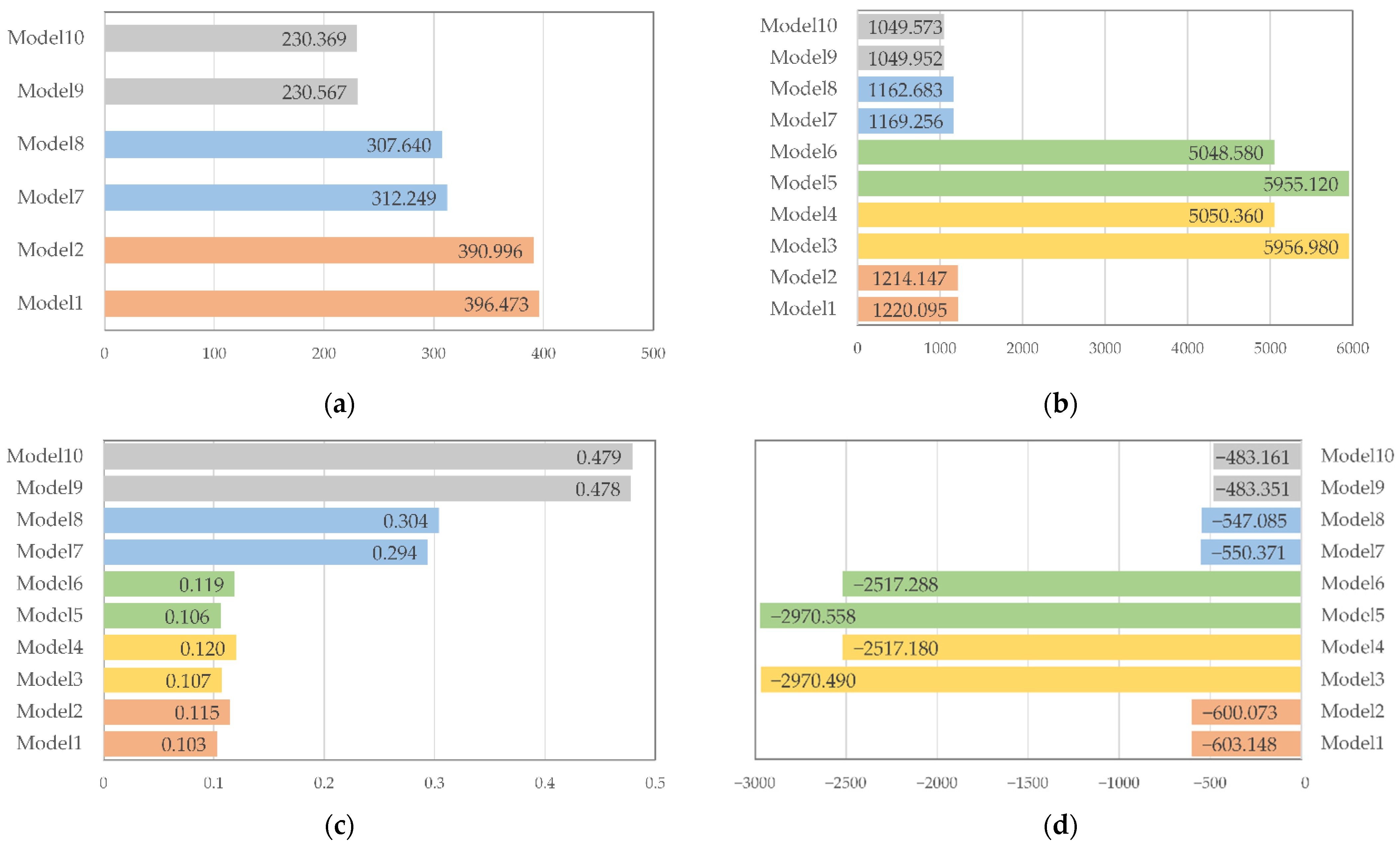
The following indexes were used to evaluate the fitness of the model: RSS, AIC, R2, and log-likelihood. For RSS and AIC, smaller values indicate better fitness. For R2 and log-likelihood, the higher the value, the better the fitness. The values of the evaluation indexes are listed in Table 4, and the comparison results of model fitting are vividly displayed using histograms in Figure 3. Taking the model for weekday crashes as an example, model 1, model 3, model 5, model 7, and model 9 were developed based on OLS, SLM, SEM, GWR, and MGWR. The value of RSS of model 9 is the lowest, indicating that the MGWR model generated the least error. The AIC value is 1049.952 in model 9, which is the lowest and indicates that the MGWR has the best data fitness. R2 describes the degree to which input variables can explain output variables and ranges from 0 to 1. The better the predictor variable in explaining the response variable, the better the fitting effect of the model. The R2 of model 9 is 0.478, which is larger than those of model 1 (0.103), model 3 (0.107), model 5 (106), and model 7 (0.297). In comparison with the fit metrics of the global regression models, the R2 value of model 9 (0.478) is the highest. In comparison with the fit metrics of the global regression models, the log-likelihood value of model 9 (−483.351) is the highest.
Collectively, the proposed method based on MGWR models outperformed the OLS, SLM, SEM, and GWR models in terms of model fitting. The proposed method not only allows the estimation parameters to vary with space but also considers the bandwidth at different scales instead of using a single average bandwidth. This means that the model’s explanatory ability and fitting effect can be further improved by optimizing the choice of bandwidth.
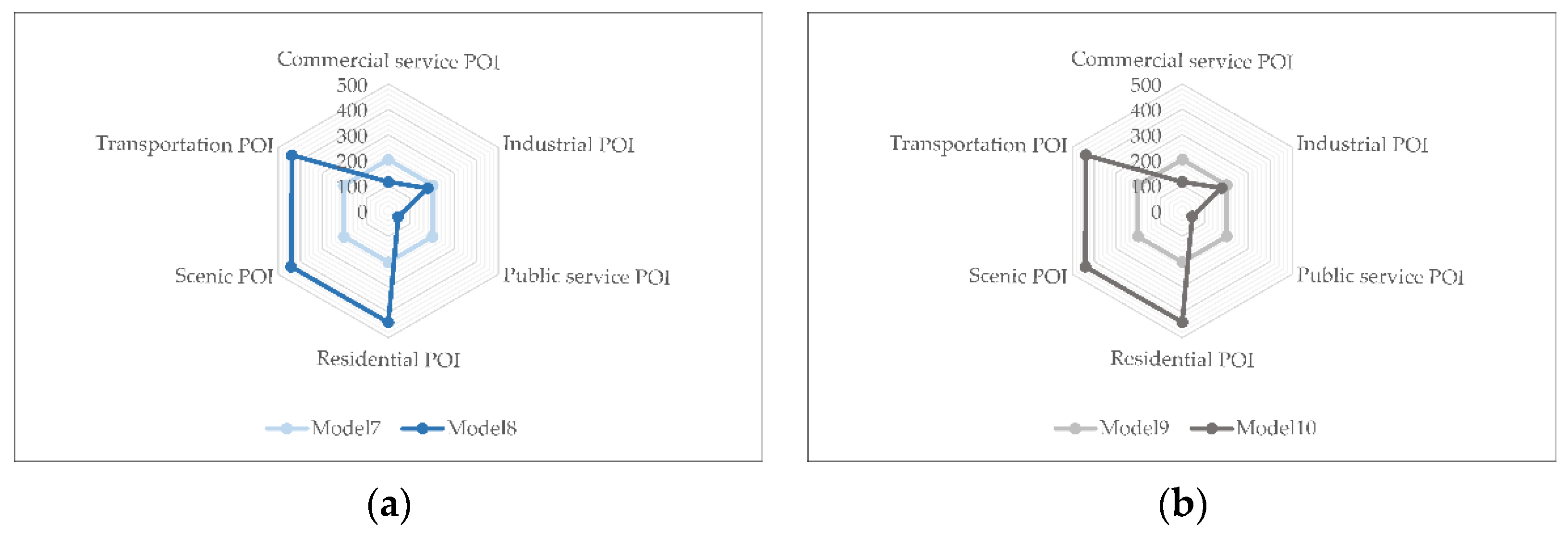
The kernel function has little influence on the regression results, while the bandwidth has significant influence. This means the bandwidth controls the smoothness of the model and is the most important parameter of the MGWR. The bandwidth of the GWR is a fixed value that only reflects the average scale of each variable, while the MGWR can reveal the different effects of various variables. MGWR relaxes the assumption that the spatial variation of different processes being modeled operate at the same spatial scale and derives optimal bandwidths for the relationships between the response variable and the different predictor variables [25]. The navy blue and dark gray lines in the two radar charts in Figure 4 show the optimal bandwidths for different predictor variables obtained by the MGWR model. The baby blue and light gray lines indicate there to be a single bandwidth for predictor variables generated by the GWR model. As shown in Table 5, the optimal bandwidth for the different variables in the MGWR varied considerably. The optimal bandwidth of public service POI was 45, which is relatively small and has strong spatial heterogeneity. It affected the occurrence of traffic crashes at the local scale, and the spatial pattern of coefficient estimates was largely different. The bandwidths of commercial service POI and industrial POI were 114 and 179, respectively, close to the average bandwidth of the GWR. The estimates for these two variables differed at the regional scale and had relative stability in space. Other variables affected traffic crashes at the global scale, and their optimal bandwidths were close to or equal to the maximum possible number of neighbors, which is 441. The influence of these variables on traffic crashes had spatial stability, and there was almost no spatial heterogeneity. The GWR model generated an optimal bandwidth of 202 for all predictor variables. This single bandwidth assumes that all variables affect the occurrence of traffic crashes at the same regional scale, which is limiting.

4.2. Results from the Proposed Method Based on MGWR

The coefficient estimate generated by the global regression model is the mean value of the study area. However, as the local spatial regression model, the local coefficient estimates generated by MGWR can reflect the spatial heterogeneity in the process of influencing traffic crashes. The results from our proposed method based on MGWR show that the relationship between the number of traffic crashes and POI in the study area changes in direction and intensity with the change of space. The influence of the same type of POI on traffic crashes may vary in different geographical locations. The mean, maximum, and minimum values of the regression coefficients for each predictor variable in the MGWR model are listed in the second to the fourth columns of Table 6. The fifth to seventh columns show the statistics of coefficient estimates based on the t-test, including the proportion of the significant estimates (p ≤ 0.05) [53], the proportion of significant positive coefficients to significant coefficients, and the proportion of significant negative coefficients to significant coefficients.
According to the t-test results in Table 6, the local coefficient estimates from residential POI and scenic POI were found to not be significant, indicating that these variables have little influence on traffic crashes. The relationship between transportation POI and traffic crashes for weekdays and weekends differs considerably. The local estimates from transportation POI are significant and positive for every community on weekends, while significant only in 15.16% of communities during weekdays. The model results also indicate some differences in the influence of transportation POI on traffic crashes at different periods and locations. About 81.25% of the local coefficient estimates in the MGWR model for weekdays are positive, while 18.75% are negative. Three-quarters of the local coefficient estimates from industrial POI in the model for weekends are significant and positive. In different communities, an increase in the number of industrial POI may increase or decrease traffic crashes. The other two variables, commercial service POI and public service POI have little and similar effects on weekday and weekend traffic crashes. In a small number of communities, the estimated values of the local coefficients are positive and significant. The more commercial service places there are, the more likely traffic crashes are to occur. The increasing number of public service facilities also increases the risk of crashes. The spatial distribution of the local coefficient estimates from MGWR models is explained below.
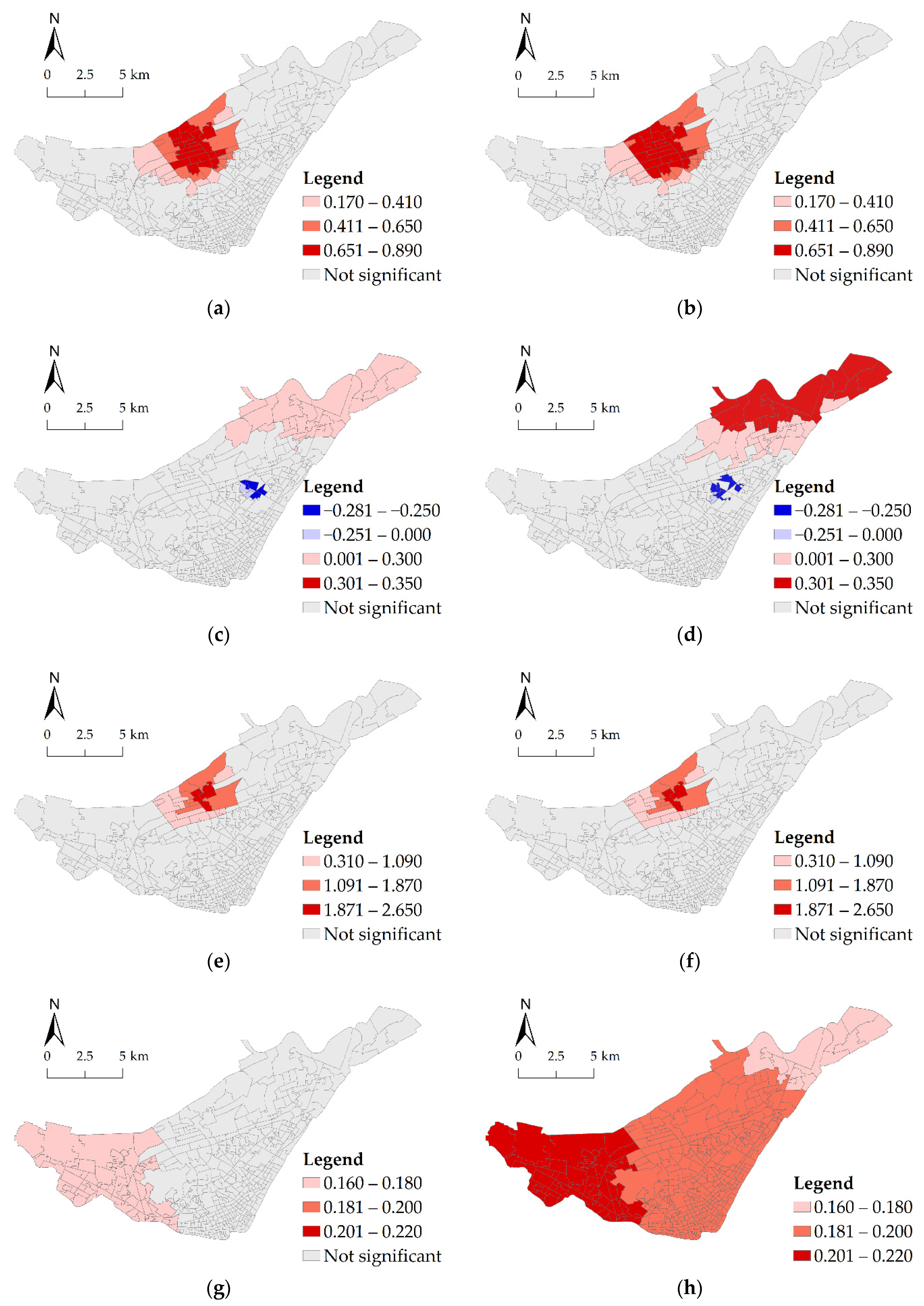
Compared with the global regression models, the main advantage of the GWR and the MGWR is that the local coefficient estimate of the predictor variables for each geographic location can be determined and visualized. ‘0’ was used as the threshold to distinguish significantly positive and negative values. The nonstationary degree of all predictor variables was tested, and the estimates were visualized as a map rendered in cool to warm colors. Figure 5a–h present the spatial distribution of the locally significant coefficient estimates.
Commercial service places are mainly related to dining and shopping activities. Prior studies have noted that commercial land attracted more pedestrians and vehicles, leading to frequent traffic crashes, especially near large commercial centers [54]. Figure 5a,b shows the MGWR coefficient results for traffic crashes, with a range of positive coefficient values located in the center of the study area, specifically in the north of Jianghan district. As shown by the spatial distribution of local coefficient estimates, the influence of commercial service POI for weekday and weekend traffic crashes is uniform. In the communities around Hankou Railway station, the local coefficient estimates were the largest, indicating that commercial service POI had the greatest impact on traffic crashes. The area around the railway station is hot spots for crashes on both weekdays and weekends. A possible explanation for this is that the traffic volume near railway stations is denser than in other areas due to the frequent population mobility.
Industrial POI mainly includes corporate enterprises and industrial parks and brings a concentration of employment. As shown in Figure 5c,d, the local coefficient estimates were positive for some areas and negative for others. Industrial POI at several central communities in Hankou had a negative impact on traffic crashes. In contrast, there was a significant positive correlation between industrial POI and crashes in the northeast area of Jiang’an district, near the Third Ring Road. This positive correlation was even stronger for weekends. With the acceleration of industrial structure adjustments in Wuhan, industrial lands in the central city have gradually transferred from the core area into the edges of the Third Ring Road. But at the same time, problems such as inadequate residential areas, deficient public service facilities, and inconvenient transportation conditions exacerbate the problem of occupational and residential separation. Long-distance travel and heavy reliance on motor vehicles increase road traffic. The industrial lands are vital in goods distribution, generating traffic volumes in non-commuting hours [55]. This may be why there was no significant difference in the influence of industrial POI on traffic crashes between weekdays and weekends.
Public service POI is generally located in areas with high population density, dense enterprises, and high accessibility to public transport. As shown in the regression results in Figure 5e,f, the coefficient estimates were all significantly positive. The spatial distribution of coefficient estimates was highly similar, indicating that the influence of public service POI on traffic crashes during weekdays and weekends is analogous. There was a higher likelihood when crashes happened on public service land both during weekdays and weekends. The optimal bandwidth of 45 reflects a local scale dimension. A significant and positive influence was present only in the northeastern Jianghan district and the northwestern Jiang’an district. The absolute value of the coefficient estimates indicates that the influence of public service on crashes is the largest among all variables. Public service places such as schools and hospitals are densely populated with people and vehicles. The possibility of traffic crashes can also be affected by temporary parking.
Transportation POI provides travel convenience for residents and is a key factor determining the travel activities of residents. In Figure 5g,h, relatively large differences in the impact of transportation POI on traffic crashes can be found at different periods. The impact of transportation POI on weekend crashes was higher than that on weekdays. The model of the impact of traffic facilities on weekend crashes suggests that the local coefficient estimates were significant and positive, ranging from 0.177 to 0.212. The optimal bandwidth of 439 indicates that the impact was at a global scale. For the entire Hankou district, the risk of traffic crashes intensified as the number of traffic facilities increases, and this positive effect was found to gradually increase from east to west of the Hankou district. On weekdays, only the traffic facilities in the Qiaokou district had a significant impact on crashes.

4.3. Discussion

This study explored the relationship between POI and traffic crashes in Hankou. Compared with the methods based on OLS, SLM, SEM, and GWR, the proposed method based on MGWR provided the most accurate coefficient estimates because it considered both spatial heterogeneity and different spatial scales of influencing factors. Some past studies [4,5] have shown that traffic crashes are more likely to occur in areas with a higher density of industrial land use. However, the research results in this study indicate that industrial land use has a positive impact on traffic crashes in some communities of the study area, while the impact of industrial land use on other communities is negative. Our proposed method can determine the local coefficient estimates of predictor variables in each unit of the study area and is better than the method based on the global regression model in explaining the spatial heterogeneity of predictor variables. From the absolute values of the local coefficient estimates, the effect of public service POI on crashes was found to be the strongest. An increase in the number of commercial service POI and public service POI increased the probability of crashes in some communities. The local coefficient estimates for residential POI and scenic POI were both not significant and had little effect on traffic crashes. The spatial scales for different predictor variables varied. Transportation POI is the most important factor in road traffic, affecting traffic safety on a global scale. Local coefficient estimates associated with transportation POI are similar across space, while the effect of public service POI on traffic crashes varies locally. Industrial lands with inadequate public service facilities and inconvenient transportation have a higher possibility of traffic crashes, and the different contributing factors affecting traffic crashes varied temporally. This finding is consistent with previous research [56,57]. During weekdays, a higher number of transportation POI caused traffic crashes for the entire study area. On the weekends, there were significant and positive effects in some communities. There was a higher likelihood when crashes happening on industrial land on weekdays than weekends. Therefore, to reduce traffic crashes, the local traffic management bureau should recognize the differences between influencing factors that cause crashes and understand the reasons for such differences.

5. Conclusions

In this paper, we developed an MGWR-based method to explore the relationship between POI and traffic crashes occurring on weekdays and weekends and compared its performance against the method based on the global regression models (OLS, SLM, and SEM), the OLS-based model, and the method based on GWR. By considering spatial heterogeneity and spatial scale differences, the proposed method significantly improves the accuracy of the regression results and is more suitable in analyzing POI influence on traffic crashes. The research results indicate that there were clear differences in the scale of the influencing factors of traffic crashes. Public service affects crashes at the local scale. From the local coefficient estimates, commercial service POI and industrial POI affect road traffic crashes at the regional scale. And other POI affect traffic crashes at a global scale. Residential POI and scenic POI had little effect on traffic crashes. This finding contradicts other research [2,6,7] that identified residential land as a major contributing factor for crashes. During weekdays, a higher number of transportation POI caused traffic crashes for the entire study area. On the weekends, there were significant and positive effects in some communities. Industrial POI was found to have positive and negative impacts on crashes in particular areas. An increase in the number of commercial service POI and public service POI increased the probability of crashes in some communities.
Compared with past studies, the innovation of this study is as follows: (1) the relationship between land use and traffic crashes can be explained from a microscopic scale by using POI data to represent the distribution characteristics of land use; (2) the proposed method based on MGWR model can effectively solve the problem of spatial heterogeneity and spatial scale difference of predictor variables; and (3) the study of POI on the impact of weekday and weekend traffic crashes provides a reliable reference for further exploring the temporal variance of the influence mechanism of traffic crashes.
At present, traffic safety is an important issue affecting public health and safety. The findings of this investigation complement those of earlier studies. However, there are still some shortcomings in this research, primarily due to limited available data. Only six categories of POI data were used as predictor variables, and other types of influencing factors were not considered. Further research is needed to include more variables in subsequent studies to help improve the accuracy of results. Future studies can also improve the calculation method and modify the model to increase its performance.

Author Contributions

Xinyu Qu proposed the idea, designed the experiments, analyzed the data, and wrote the manuscript; Xiongwu Xiao, Deren Li, Huayi Wu, Bingxuan Guo, and Xinyan Zhu revised the manuscript and offered substantial improvement for this paper. All authors have read and agreed to the published version of the manuscript.

Funding

This research was funded by the National Natural Science Foundation of China (Grant Nos. 42101449, 91638203, 91738302), the Chutian Scholar Program of Hubei Province, the Yellow Crane Talent Scheme, the Natural Science Foundation of Hubei Province of China (Grant No. 2020CFA001), the Science and Technology Program of Southwest China Research Institute of Electronic Equipment (Grant No. JS20200500114), Fundamental Research Funds for the Central Universities of China (Grant No. 2042019kf0002), the Science and Technology Program of Guangzhou, China (Grant No. 2017010160173) and LIESMARS Special Research Funding.

Institutional Review Board Statement

Not applicable.

Informed Consent Statement

Not applicable.

Data Availability Statement

The traffic crash data used in this work are party data that are owned by the Wuhan Traffic Management Bureau in China (http://www.whjg.gov.cn). The Wuhan Traffic Management Bureau in China cannot make these collision data publicly available due to legal restrictions.

Acknowledgments

We would like to thank the reviewers for their comments and nice suggestions, which greatly improved the manuscript.

Conflicts of Interest

The authors declare no conflict of interest.

Abbreviations

MGWRMultiscale geographically weighted regression [25]
POIPoint-of-interest
OLSOrdinary least squares [41]
SLMSpatial lag model [42]
SEMSpatial error model [42]
GWRGeographically weighted regression [13]
VIFVariance inflation factor
AICAkaike information criterion [45]
AICcCorrected Akaike information criterion [45,46]
GAMGeneralized additive model [48]
RSSResidual sum of squares

References

  1. World Health Organization. World Health Statistics 2020: Monitoring Health for the SDGs, Sustainable Development Goals; World Health Organization: Geneva, Switzerland, 2020; ISBN 978-92-4-000510-5. [Google Scholar]
  2. Pulugurtha, S.S.; Duddu, V.R.; Kotagiri, Y. Traffic Analysis Zone Level Crash Estimation Models Based on Land Use Characteristics. Accid. Anal. Prev. 2013, 50, 678–687. [Google Scholar] [CrossRef] [PubMed]
  3. Xu, C.; Wang, Y.; Ding, W.; Liu, P. Modeling the Spatial Effects of Land-Use Patterns on Traffic Safety Using Geographically Weighted Poisson Regression. Netw. Spat. Econ. 2020, 20, 1015–1028. [Google Scholar] [CrossRef]
  4. Levine, N.; Kim, K.E.; Nitz, L.H. Spatial Analysis of Honolulu Motor Vehicle Crashes: I. Spatial Patterns. Accid. Anal. Prev. 1995, 27, 663–674. [Google Scholar] [CrossRef]
  5. Ukkusuri, S.; Miranda-Moreno, L.F.; Ramadurai, G.; Isa-Tavarez, J. The Role of Built Environment on Pedestrian Crash Frequency. Saf. Sci. 2012, 50, 1141–1151. [Google Scholar] [CrossRef]
  6. Kim, K.; Pant, P.; Yamashita, E. Accidents and Accessibility: Measuring Influences of Demographic and Land Use Variables in Honolulu, Hawaii. Transp. Res. Rec. 2010, 2147, 9–17. [Google Scholar] [CrossRef]
  7. Xie, B.; An, Z.; Zheng, Y.; Li, Z. Incorporating Transportation Safety into Land Use Planning: Pre-Assessment of Land Use Conversion Effects on Severe Crashes in Urban China. Appl. Geogr. 2019, 103, 1–11. [Google Scholar] [CrossRef]
  8. Miranda-Moreno, L.F.; Morency, P.; El-Geneidy, A.M. The Link between Built Environment, Pedestrian Activity and Pedestrian–Vehicle Collision Occurrence at Signalized Intersections. Accid. Anal. Prev. 2011, 43, 1624–1634. [Google Scholar] [CrossRef] [PubMed]
  9. Hadayeghi, A.; Shalaby, A.; Persaud, B. Development of Planning-Level Transportation Safety Models Using Full Bayesian Semiparametric Additive Techniques. J. Transp. Saf. Secur. 2010, 2, 45–68. [Google Scholar] [CrossRef]
  10. Narayanamoorthy, S.; Paleti, R.; Bhat, C.R. On Accommodating Spatial Dependence in Bicycle and Pedestrian Injury Counts by Severity Level. Transp. Res. Part B Methodol. 2013, 55, 245–264. [Google Scholar] [CrossRef] [Green Version]
  11. Kim, K.; Yamashita, E. Motor Vehicle Crashes and Land Use: Empirical Analysis from Hawaii. Transp. Res. Rec. 2002, 1784, 73–79. [Google Scholar] [CrossRef]
  12. Jia, R.; Khadka, A.; Kim, I. Traffic Crash Analysis with Point-of-Interest Spatial Clustering. Accid. Anal. Prev. 2018, 121, 223–230. [Google Scholar] [CrossRef]
  13. Stewart Fotheringham, A.; Charlton, M.; Brunsdon, C. The Geography of Parameter Space: An Investigation of Spatial Non-Stationarity. Int. J. Geogr. Inf. Syst. 1996, 10, 605–627. [Google Scholar] [CrossRef]
  14. Erdogan, S. Explorative Spatial Analysis of Traffic Accident Statistics and Road Mortality among the Provinces of Turkey. J. Saf. Res. 2009, 40, 341–351. [Google Scholar] [CrossRef]
  15. Rhee, K.-A.; Kim, J.-K.; Lee, Y.; Ulfarsson, G.F. Spatial Regression Analysis of Traffic Crashes in Seoul. Accid. Anal. Prev. 2016, 91, 190–199. [Google Scholar] [CrossRef]
  16. Li, Z.; Wang, W.; Liu, P.; Bigham, J.M.; Ragland, D.R. Using Geographically Weighted Poisson Regression for County-Level Crash Modeling in California. Saf. Sci. 2013, 58, 89–97. [Google Scholar] [CrossRef]
  17. Pirdavani, A.; Bellemans, T.; Brijs, T.; Wets, G. Application of Geographically Weighted Regression Technique in Spatial Analysis of Fatal and Injury Crashes. J. Transp. Eng. 2014, 140, 04014032. [Google Scholar] [CrossRef]
  18. Shariat-Mohaymany, A.; Shahri, M.; Mirbagheri, B.; Matkan, A.A. Exploring Spatial Non-Stationarity and Varying Relationships between Crash Data and Related Factors Using Geographically Weighted Poisson Regression: Non-Stationarity and Varying Relationships between Crash Data and Related Factors. Trans. GIS 2015, 19, 321–337. [Google Scholar] [CrossRef]
  19. Hezaveh, A.M.; Arvin, R.; Cherry, C.R. A Geographically Weighted Regression to Estimate the Comprehensive Cost of Traffic Crashes at a Zonal Level. Accid. Anal. Prev. 2019, 131, 15–24. [Google Scholar] [CrossRef]
  20. Gomes, M.J.T.L.; Cunto, F.; da Silva, A.R. Geographically Weighted Negative Binomial Regression Applied to Zonal Level Safety Performance Models. Accid. Anal. Prev. 2017, 106, 254–261. [Google Scholar] [CrossRef]
  21. Liu, J.; Khattak, A.J.; Wali, B. Do Safety Performance Functions Used for Predicting Crash Frequency Vary across Space? Applying Geographically Weighted Regressions to Account for Spatial Heterogeneity. Accid. Anal. Prev. 2017, 109, 132–142. [Google Scholar] [CrossRef]
  22. Obelheiro, M.R.; da Silva, A.R.; Nodari, C.T.; Cybis, H.B.B.; Lindau, L.A. A New Zone System to Analyze the Spatial Relationships between the Built Environment and Traffic Safety. J. Transp. Geogr. 2020, 84, 102699. [Google Scholar] [CrossRef]
  23. Wang, C.; Li, S.; Shan, J. Non-Stationary Modeling of Microlevel Road-Curve Crash Frequency with Geographically Weighted Regression. ISPRS Int. J. Geo-Inf. 2021, 10, 286. [Google Scholar] [CrossRef]
  24. Tang, J.; Gao, F.; Liu, F.; Han, C.; Lee, J. Spatial Heterogeneity Analysis of Macro-Level Crashes Using Geographically Weighted Poisson Quantile Regression. Accid. Anal. Prev. 2020, 148, 105833. [Google Scholar] [CrossRef]
  25. Fotheringham, A.S.; Yang, W.; Kang, W. Multiscale Geographically Weighted Regression (MGWR). Ann. Am. Assoc. Geogr. 2017, 107, 1247–1265. [Google Scholar] [CrossRef]
  26. Mollalo, A.; Vahedi, B.; Rivera, K.M. GIS-Based Spatial Modeling of COVID-19 Incidence Rate in the Continental United States. Sci. Total Environ. 2020, 728, 138884. [Google Scholar] [CrossRef]
  27. Maiti, A.; Zhang, Q.; Sannigrahi, S.; Pramanik, S.; Chakraborti, S.; Cerda, A.; Pilla, F. Exploring Spatiotemporal Effects of the Driving Factors on COVID-19 Incidences in the Contiguous United States. Sustain. Cities Soc. 2021, 68, 102784. [Google Scholar] [CrossRef] [PubMed]
  28. Mansour, S.; Al Kindi, A.; Al-Said, A.; Al-Said, A.; Atkinson, P. Sociodemographic Determinants of COVID-19 Incidence Rates in Oman: Geospatial Modelling Using Multiscale Geographically Weighted Regression (MGWR). Sustain. Cities Soc. 2021, 65, 102627. [Google Scholar] [CrossRef]
  29. Wu, C.; Ren, F.; Hu, W.; Du, Q. Multiscale Geographically and Temporally Weighted Regression: Exploring the Spatiotemporal Determinants of Housing Prices. Int. J. Geogr. Inf. Sci. 2019, 33, 489–511. [Google Scholar] [CrossRef]
  30. Tomal, M. Exploring the Meso-Determinants of Apartment Prices in Polish Counties Using Spatial Autoregressive Multiscale Geographically Weighted Regression. Appl. Econ. Lett. 2021, 1–9. [Google Scholar] [CrossRef]
  31. Fotheringham, A.S.; Yue, H.; Li, Z. Examining the Influences of Air Quality in China’s Cities Using Multi-scale Geographically Weighted Regression. Trans. GIS 2019, 23, 1444–1464. [Google Scholar] [CrossRef]
  32. Fan, Z.; Zhan, Q.; Yang, C.; Liu, H.; Zhan, M. How Did Distribution Patterns of Particulate Matter Air Pollution (PM 2.5 and PM 10) Change in China during the COVID-19 Outbreak: A Spatiotemporal Investigation at Chinese City-Level. Int. J. Environ. Res. Public Health 2020, 17, 6274. [Google Scholar] [CrossRef]
  33. Yan, J.-W.; Tao, F.; Zhang, S.-Q.; Lin, S.; Zhou, T. Spatiotemporal Distribution Characteristics and Driving Forces of PM2.5 in Three Urban Agglomerations of the Yangtze River Economic Belt. Int. J. Environ. Res. Public Health 2021, 18, 2222. [Google Scholar] [CrossRef]
  34. Stewart Fotheringham, A.; Li, Z.; Wolf, L.J. Scale, Context, and Heterogeneity: A Spatial Analytical Perspective on the 2016 U.S. Presidential Election. Ann. Am. Assoc. Geogr. 2021, 1–20. [Google Scholar] [CrossRef]
  35. Zhang, L.; Cheng, J.; Jin, C.; Zhou, H. A Multiscale Flow-Focused Geographically Weighted Regression Modelling Approach and Its Application for Transport Flows on Expressways. Appl. Sci. 2019, 9, 4673. [Google Scholar] [CrossRef] [Green Version]
  36. Iyanda, A.E.; Osayomi, T. Is There a Relationship between Economic Indicators and Road Fatalities in Texas? A Multiscale Geographically Weighted Regression Analysis. GeoJournal 2021, 86, 2787–2807. [Google Scholar] [CrossRef]
  37. Erdogan, S.; Yilmaz, I.; Baybura, T.; Gullu, M. Geographical Information Systems Aided Traffic Accident Analysis System Case Study: City of Afyonkarahisar. Accid. Anal. Prev. 2008, 40, 174–181. [Google Scholar] [CrossRef] [PubMed]
  38. Yu, R.; Abdel-Aty, M. Investigating the Different Characteristics of Weekday and Weekend Crashes. J. Saf. Res. 2013, 46, 91–97. [Google Scholar] [CrossRef] [PubMed]
  39. Anowar, S.; Yasmin, S.; Tay, R. Comparison of Crashes during Public Holidays and Regular Weekends. Accid. Anal. Prev. 2013, 51, 93–97. [Google Scholar] [CrossRef]
  40. Yue, H.; Zhu, X.; Ye, X.; Guo, W. The Local Colocation Patterns of Crime and Land-Use Features in Wuhan, China. ISPRS Int. J. Geo-Inf. 2017, 6, 307. [Google Scholar] [CrossRef] [Green Version]
  41. Anselin, L.; Bera, A.K.; Florax, R.; Yoon, M.J. Simple Diagnostic Tests for Spatial Dependence. Reg. Sci. Urban Econ. 1996, 26, 77–104. [Google Scholar] [CrossRef]
  42. Anselin, L.; Rey, S. Properties of Tests for Spatial Dependence in Linear Regression Models. Geogr. Anal. 2010, 23, 112–131. [Google Scholar] [CrossRef]
  43. Pellegrini, P.A.; Fotheringham, A.S. Modelling Spatial Choice: A Review and Synthesis in a Migration Context. Prog. Hum. Geogr. 2002, 26, 487–510. [Google Scholar] [CrossRef]
  44. Murakami, D.; Lu, B.; Harris, P.; Brunsdon, C.; Charlton, M.; Nakaya, T.; Griffith, D.A. The Importance of Scale in Spatially Varying Coefficient Modeling. Ann. Am. Assoc. Geogr. 2019, 109, 50–70. [Google Scholar] [CrossRef]
  45. Akaike, H. Factor Analysis and AIC. In Selected Papers of Hirotugu Akaike; Springer: New York, NY, USA, 1987. [Google Scholar]
  46. Sugiura, N. Further Analysts of the Data by Akaike’s Information Criterion and the Finite Corrections: Further Analysts of the Data by Akaike’ s. Commun. Stat.-Theory Methods 1978, 7, 13–26. [Google Scholar] [CrossRef]
  47. Yang, W. An Extension of Geographically Weighted Regression with Flexible Bandwidths. Ph.D. Thesis, University of St Andrews, St Andrews, Scotland, UK, 2014. [Google Scholar]
  48. Hastie, T.; Tibshirani, R. Generalized Additive Models: Some Applications. J. Am. Stat. Assoc. 1987, 82, 371–386. [Google Scholar] [CrossRef]
  49. Buja, A.; Hastie, T.; Tibshirani, R. Linear Smoothers and Additive Models. Ann. Statist. 1989, 17, 453–510. [Google Scholar] [CrossRef]
  50. Wolf, L.J.; Oshan, T.M.; Fotheringham, A.S. Single and Multiscale Models of Process Spatial Heterogeneity: Single and Multiscale Models. Geogr. Anal. 2018, 50, 223–246. [Google Scholar] [CrossRef] [Green Version]
  51. Oshan, T.; Li, Z.; Kang, W.; Wolf, L.; Fotheringham, A. Mgwr: A Python Implementation of Multiscale Geographically Weighted Regression for Investigating Process Spatial Heterogeneity and Scale. ISPRS Int. J. Geo-Inf. 2019, 8, 269. [Google Scholar] [CrossRef] [Green Version]
  52. Anselin, L.; Syabri, I.; Kho, Y.A. GeoDa: An Introduction to Spatial Data Analysis. In Handbook of Applied Spatial Analysis; Springer: Berlin/Heidelberg, Germany, 2010. [Google Scholar]
  53. Wang, P.; Ren, H.; Zhu, X.; Fu, X.; Liu, H.; Hu, T. Spatiotemporal Characteristics and Factor Analysis of SARS-CoV-2 Infections among Healthcare Workers in Wuhan, China. J. Hosp. Infect. 2021, 110, 172–177. [Google Scholar] [CrossRef]
  54. Huang, Y.; Wang, X.; Patton, D. Examining Spatial Relationships between Crashes and the Built Environment: A Geographically Weighted Regression Approach. J. Transp. Geogr. 2018, 69, 221–233. [Google Scholar] [CrossRef]
  55. Priyantha Wedagama, D.M.; Bird, R.N.; Metcalfe, A.V. The Influence of Urban Land-Use on Non-Motorised Transport Casualties. Accid. Anal. Prev. 2006, 38, 1049–1057. [Google Scholar] [CrossRef] [PubMed]
  56. Adanu, E.K.; Hainen, A.; Jones, S. Latent Class Analysis of Factors That Influence Weekday and Weekend Single-Vehicle Crash Severities. Accid. Anal. Prev. 2018, 113, 187–192. [Google Scholar] [CrossRef] [PubMed]
  57. Song, L.; Li, Y.; Fan, W.; Liu, P. Mixed Logit Approach to Analyzing Pedestrian Injury Severity in Pedestrian-Vehicle Crashes in North Carolina: Considering Time-of-Day and Day-of-Week. Traffic Inj. Prev. 2021, 22, 524–529. [Google Scholar] [CrossRef] [PubMed]
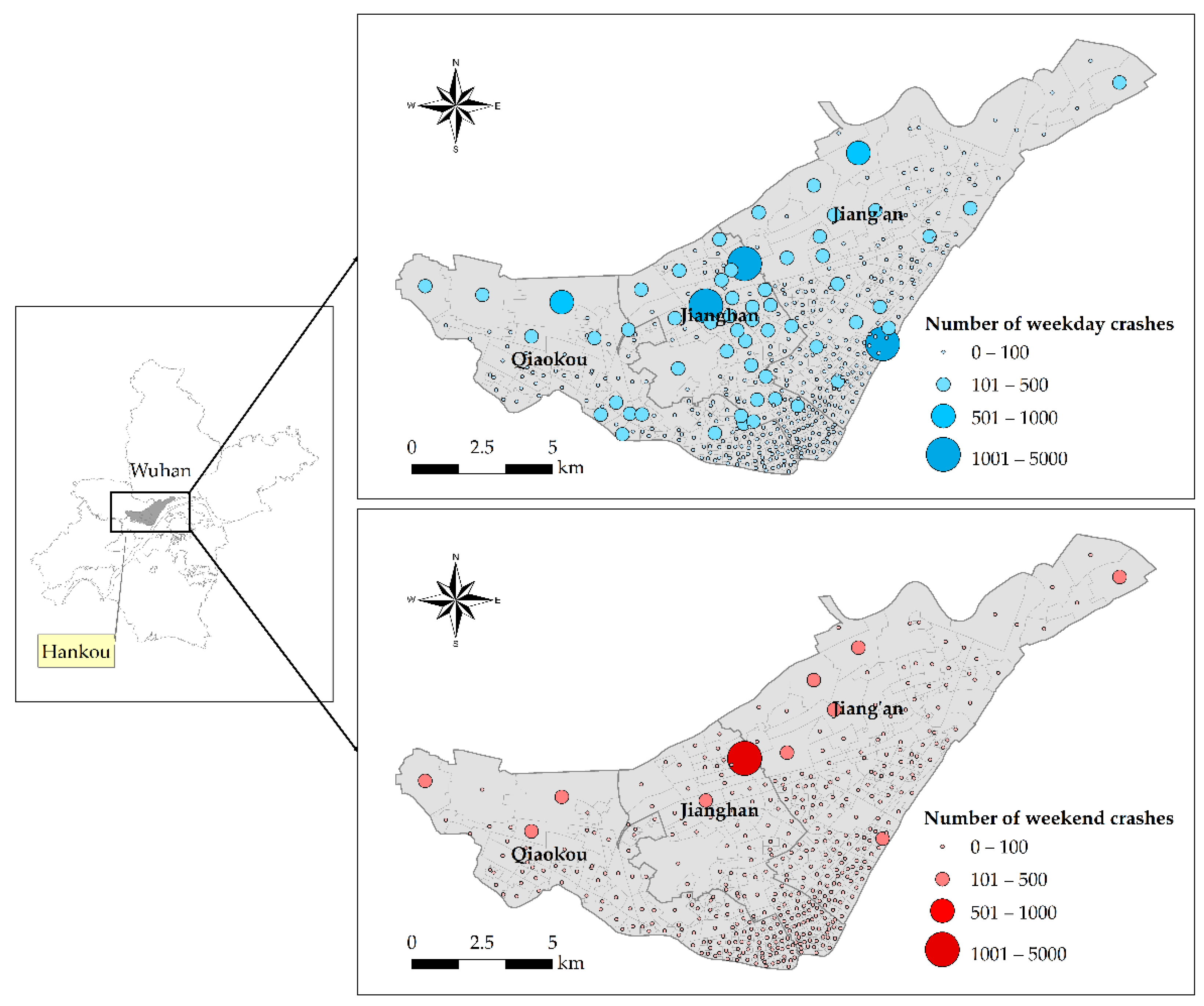
Figure 1. Location of the study area and spatial distribution of the number of traffic crashes per community.
Ijgi 10 00791 g001
Figure 2. Flowchart of our study.
Ijgi 10 00791 g002
Figure 3. Comparison of the evaluation indexes of the 10 models. (a) Residual sum of squares (RSS); (b) Akaike information criterion (AIC); (c) R-squared (R2); (d) Log-likelihood.
Ijgi 10 00791 g003
Figure 4. Comparison of the bandwidths of the geographically weighted regression (GWR) and multi-scale geographically weighted regression (MGWR) models. (a) The bandwidths of model7 and model8; (b) The bandwidths of model9 and model10.
Ijgi 10 00791 g004
Figure 5. The spatial distribution of local coefficient estimates from MGWR models. (a) Model9 results for commercial service POI; (b) Model10 results for commercial service POI; (c) Model9 results for industrial POI; (d) Model10 results for industrial POI; (e) Model9 results for public service POI; (f) Model10 results for public service POI; (g) Model9 results for transportation POI; (h) Model10 results for transportation POI.
Ijgi 10 00791 g005
Table 1. Reclassification results of points-of-interest (POI) data.
CategoryNarrowed Category
Residential POICommercial house, residential area
Commercial service POITea house; bakery, coffee house, fast food restaurant, ice cream shop, dessert house, foreign food restaurant, leisure food restaurant, Chinese food restaurant, convenience store, supermarket, clothing store, personal care items shop, plants and pet market, home electronics hypermarket, home building materials market, shopping plaza, commercial street, sports store, stationery store, franchise store, comprehensive market, hotel, hostel, insurance company, finance company, finance and insurance service institution, bank, securities company, ATM, sports and recreation places, recreation place, theatre, cinema, recreation center
Industrial POIFactory, company, enterprises, farming, forestry, animal husbandry and fishery base, industrial park
Transportation POISubway station, port, marina, bus station, railway station, ferry station, parking lot, coach station
Scenic POIScenery spot, park, square
Public service POITraining institution, museum, archives hall, driving school, science and technology museum, science and education cultural place, research institution, art gallery, library, cultural palace, school, exhibition hall, hospital, special hospital, emergency center, disease prevention institution, industrial and commercial taxation institution, public security organization, traffic vehicle management, social group, governmental organization, social groups, holiday and nursing resort, sports stadium
Table 2. Descriptive statistics of response and predictor variables based on communities.
VariablesMeanStd. Dev.Min.Max.VIF
Response variablesNumber of crashes on weekdays63.08212.4603877-
Number of crashes on weekends23.3676.7401365-
Predictor
variables
Number of commercial service POI191.89247.91024091.56
Number of industrial POI30.7255.4704502.47
Number of public service POI26.3925.2201583.11
Number of residential POI9.128.790642.02
Number of scenic POI1.318.5801671.19
Number of transportation POI15.5918.8601364.03
Table 3. Description of the ten regression models.
ModelsDescription of the Models
Model 1The global regression model of POI and weekday crashes based on the OLS method.
Model 2The global regression model of POI and weekend crashes based on the OLS method.
Model 3The global regression model of POI and weekday crashes based on the SLM model.
Model 4The global regression model of POI and weekend crashes based on the SLM model.
Model 5The global regression model of POI and weekday crashes based on the SEM model.
Model 6The global regression model of POI and weekend crashes based on the SEM model.
Model 7The local regression model of POI and weekday crashes based on the GWR method.
Model 8The local regression model of POI and weekend crashes based on the GWR method.
Model 9The local regression model of POI and weekday crashes based on the MGWR method.
Model 10The local regression model of POI and weekend crashes based on the MGWR method.
Table 4. The goodness of fit statistics for the 10 models.
ModelsEvaluate Indexes
RSSAICR2Log-Likelihood
OLSModel 1396.4731220.0950.103−603.148
Model 2390.9961214.1470.115−600.073
SLMModel 3-5956.9800.107−2970.490
Model 4-5050.3600.120−2517.180
SEMModel 5-5955.1200.106−2970.558
Model 6-5048.5800.119−2517.288
GWRModel 7312.2491169.2560.294−550.371
Model 8307.6401162.6830.304−547.085
MGWRModel 9230.5671049.9520.478−483.351
Model 10230.3691049.5730.479−483.161
Table 5. Multi-scale bandwidth comparison of the GWR and MGWR models.
Predictor VariablesBandwidths
Model 7Model 8Model 9Model 10
Intercept--442.000442.000
Commercial service POI202.000202.000114.000114.000
Industrial POI202.000202.000179.000179.000
Public service POI202.000202.00045.00045.000
Residential POI202.000202.000439.000439.000
Scenic POI202.000202.000441.000441.000
Transportation POI202.000202.000439.000439.000
Table 6. Summary statistics for the MGWR coefficient estimates.
Predictor VariablesModel 9Model 10
MGWR CoefficientsPercentage of Communities by Significance (95% Level) of t-TestMGWR CoefficientsPercentage of Communities by Significance (95% Level) of t-Test
MeanMinMaxp ≤ 0.05 (%)+ (%)− (%)MeanMinMaxp ≤ 0.05 (%)+ (%)− (%)
Intercept−0.044−0.0670.022000−0046−0.0720.027000
Commercial service POI0.094−0.0440.86310.8610000.116−0.0320.88111.091000
Industrial POI−0.013−0.2690.2937.2481.2518.75−0.025−0.2810.3479.957525
Public service POI0.093−0.2532.6445.6610000.079−0.2682.5335.431000
Residential POI−0.046−0.062−0.041000−0.047−0.062−0.042000
Scenic POI0.0810.0750.0870000.0720.0670.079000
Transportation POI0.1620.1440.17915.1610000.1920.1770.2121001000
Publisher’s Note: MDPI stays neutral with regard to jurisdictional claims in published maps and institutional affiliations.