Abstract
The importance of combining spatial and temporal aspects has been increasingly recognized over recent years, yet pertinent pattern analysis methods in place-based crime research still need further development to explicitly indicate spatial-temporal localities of pertinent factors’ influence ranges. This paper proposes an approach, Spatial-Temporal Indication of Crime Association (STICA), to facilitate identifying the main contributing factors of crime, which are operated at diverse spatial-temporal scales. The method’s rationale is to progressively discern the spatial zones with diverse temporal crime patterns. A specific implementation of the STICA approach, by combining kernel density estimation, k-median-centers clustering, and thematic mapping, is applied to understand the burglary in an urban peninsula, China. The empirical findings include: (1) both the main time-stable and time-varying factors of crime can be indicated with the disparities of temporal crime patterns for different spatial zones based on the STICA results. (2) The spatial range of these factors can enlighten the understanding of interactions for generating crime patterns, especially with regards to how temporally transient and spatially global factors can produce a locally crime-ridden zone through the mediation of stable factors. (3) The STICA results can reveal the spatially contextual effects of stable factors, which are of great value to improve modeling crime patterns. As demonstrated, the STICA approach is effective in exploring contributing factors of crime and has shown great potential for providing a new vision in place-based crime research.
1. Introduction
Crime is one of the most striking problems in human society, and attracts considerable attention from many scholars and practitioners, who focus on distinct aspects (e.g., social, economic, psychological) [1]. Among these, the geographical perspective has played an increasingly critical role in understanding crime occurrence mechanisms and elaborating crime prevention strategies since the 1830s [2,3,4,5,6,7,8,9]. One of the most notable findings in the geographic studies of crime is that crime events are not evenly distributed in space [10,11], and usually cluster in a small discrete area with hotspots existed [12,13,14]. As extensive empirical evidence has revealed the importance of place in policing, place-based research on crime has gained worldwide recognition, especially in Western countries (e.g., America, England, Canada) [15]. However, although space and time are both fundamental attributes of objects, the combination of spatial and temporal dimensions has not been given proportionate attention in place-based crime research, when compared with the spatial aspect [16].
There are many critical reasons for combining the spatial and temporal dimensions in place-based crime research. On the one hand, from a practitioner’s perspective, the prerequisite of a place-based strategy is that the spatial crime pattern identified in the previous period will last into the next period. In other words, the spatial crime patterns are supposed to be stable over time [17,18]. However, some studies found that both stable and fluid hotspots exist simultaneously within a specific area [19,20]. When the spatial-temporal scale of measurement decreases, the crime hotspots become more dynamic and less stable [21]. If crime prevention resources are devoted to the fluid hotspots, this would cause great wastes of resources, while producing little or even no crime deterrence effect. For a specific crime prevention strategy to be effective and efficient, the temporal evolvement of spatial crime patterns needs to be addressed beforehand. On the other hand, from a researcher’s perspective, crime is the result of complex interactions among offenders, victims, and guardians [22,23], which are all under the influence of various underlying factors, such as the physical environment, movement rhythm, and special events [24,25]. Most factors are unevenly distributed in space and have a limited influence range. Some factors are stable, producing an unevenly spatial crime pattern without any temporal fluctuations, while some factors are time-varying, producing an uneven crime distribution in both space and time. How to identify and discriminate these types of factors is important for unraveling underlying mechanisms of crime patterns. As demonstrated in this article, when the spatial and temporal aspects of crime are taken into account simultaneously, insightful knowledge can be gained to cope with this issue.
Whether the focus is developing place-based interventions or understanding crime occurrence, the fundamental issue that has to be addressed is to identify and distinguish meaningful crime patterns, which can indicate the influence factors of crime events with diverse influence ranges in space and varying moments and durations in time. However, as suggested in the following literature review, previous spatial-temporal analysis methods in crime research have many limitations in answering this question. As a result, this paper will focus on this basic question and propose a novel approach of Spatial-Temporal Indication of Crime Association (STICA), which can enlighten the determination of possible principal influence factors of crime and their influence ranges both in space and time. This is done by differentiating crime spaces with diverse temporal patterns. The feasibility and effectiveness of this approach for shedding light on understanding crime mechanisms are demonstrated with an empirical case study of the burglary in an urban peninsula, China.
Overall, this study contributes to the literature in at least three aspects. First, as the factors affecting crime are tremendous, the STICA approach can facilitate the identification of both time-stable and time-varying factors by providing a graphical indication of the temporal disparities of crime levels for different spatial zones. Second, the STICA approach can advance our understanding of the crime occurrence mechanism by revealing how a spatially global and temporally transient factor produces a locally crime-ridden zone. Third, this paper provides an innovative way of statistically modeling crime patterns by incorporating the spatially contextual information reflected in the STICA result, which may reveal the behavioral settings of offenders.
Considering that this work belongs to the broad category of spatial-temporal pattern recognitions, we begin with a systematic review of the spatial-temporal analysis methods commonly used in place-based crime research. Thereafter, the theoretical basis and conceptual framework of this novel approach are proposed, followed by a specific implementation of the STICA approach. Subsequently, a brief introduction of the available data in the study area is provided, and the spatial-temporal patterns of crime are detected, explained, and discussed. Finally, this article concludes with a discussion of the results and their implications for future research.
2. Spatial-Temporal Analysis Methods in Place-Based Crime Research
The spatial analysis in crime research has had great breakthroughs since the 1990s, with the improvement of computing power and the enhancement of understanding crime mechanisms [12,26]. A comprehensive overview of pertinent research can be found in the work of Anselin et al. (2000) [27]. While the identification of spatial patterns keeps playing its vital role in crime research [28], the spatial-temporal crime patterns have received increasing attention over recent years [29,30,31]. Several reviews about the spatial-temporal methods for crime analysis have been conducted [32,33].
Based on the way of combining spatial and temporal dimensions in the calculating process rather than the result-presenting process, previous spatial-temporal techniques for analyzing crime patterns can be categorized into two types: one is space-time-separated and the other is space-time-integrated.
Space-time-separated approaches commonly begin with depicting spatial crime patterns and then explore their temporal variations, which means that the spatial and temporal dimensions are not integrated. The main methods of this type include map animation, comap, hotspot matrix, hotspot plot, coefficient of variation (COV), correlation analysis, etc. [16,19,20,30,34,35,36]. Map animation utilizes a consecutive series of snapshots to display temporal variations of the spatial patterns of crime [34], while comap constructs temporal bar charts and spatial maps in a matrix style, such that each map represents the distribution of crime at a specific temporal situation or a particular combination of two temporal conditions [35]. Both map animation and comap are relatively simple to create and easy to understand, but they are not effective to explore the spatial crime patterns in multiple temporal periods, and whether the spatial-temporal patterns of crime can be visually detected depends to some extent on the professionalism of users [30]. Hotspot matrix comprises two elements respectively displaying the spatial types (e.g., dispersed, clustered, and hotpoint) and the temporal types (e.g., diffused, focused, and acute) of hotspots [12], while a hotspot plot consists of three components correspondingly representing the weekly fluctuations of crime during the research period, the temporal variations of crime during the day, and the spatial patterns of crime in hotspots [16]. Both the hotspot matrix and hotspot plot are useful to discover the spatial-temporal variations within hotspots, as well as to compare the differences between hotspots; yet, both methods are not designed to deal with the whole crime patterns in the study area. COV analysis is used to determine whether or not crime hotspots are stable via measuring the fluctuation of crime intensity through time in spatial units [20]; however, a high COV value may be misleading as it does not necessarily mean a more fluctuated temporal distribution of crime levels. Instead, it can be a mostly stable temporal crime trend with a few extreme values. The correlation analysis measures the similarity of spatial patterns between any two periods [19]; yet, as a global index, it cannot capture the temporal trend of specific areas.
Space-time-integrated approaches integrate the spatial and temporal dimensions in modeling spatial-temporal patterns of crime. This approach generally includes the isosurface, space-time cube, Knox testing, spatial-temporal data mining, mathematical simulation, etc. [30,37,38,39,40]. Isosurface calculates the spatial-temporal kernel density based on crime incidents with space-time coordinates (x, y, t) [30]. This technique is very helpful to understand how the spatial patterns of crime evolve over a period of time; however, due to the difficulty of the three-dimensional display, only one specific value of isosurface can be shown at a time [30]. A space-time cube further utilizes the space-time kernel density estimation with scan statistics to generate a three-dimensional view to differentiate stable and instant crime hotspots as well as demonstrate the internal temporal variations in crime hotspots [39]. Results can be intuitively visualized, but it is not widely implemented, as the process for yielding meaningful results is difficult to handle. Knox testing identifies crime clusters by comparing the observed and expected numbers of crime in a specific space-time interval [40]. It is widely used in the identification of near-repeat crimes, but the selection of spatial and temporal scales is relatively arbitrary without clear criteria. Recently, the spatial association rules mining has been innovatively applied to analyze the spatial interactions of near-repeat crimes [41]. It can delineate the anisotropic features of the spatial interaction, while it focuses more on the spatial than the temporal dimension. The mathematical simulation reproduces the spatial-temporal process of criminal activities and crime risk based on specific models via (partial) differential equations [37,38]; it provides in-depth examinations for the mechanism of criminal activities, but is highly sophisticated and cannot be easily manipulated by most crime researchers.
In summary, noteworthy methodological achievements have been made to identify the spatial-temporal patterns of crime, but the complicated processing and the complex visualization of many techniques have, to some extent, hindered their wide application in crime prevention practice and policing management. Most geographic phenomena are dynamic and complex, and have hierarchical relationships [42]. However, the results of previous methods fail to indicate the hierarchical relationships among pertinent factors that have diverse influence ranges in space and time. Therefore, this research presents a new exploratory approach with practical potentials in the support of visualizing crime patterns and indicating the associating factors of crime.
3. Materials and Methods
3.1. Theoretical Basis of the STICA Approach
To understand crime patterns in space and time, several criminological theories are often referred to: rational choice perspective [43], routine activity approach [22], crime pattern theory [44], (temporal) constraint theory [45], and opportunity theory [46]. From an ecological perspective, crime is the result of convergences of motivated offenders, suitable targets, and incapable guardians in a specific place [22]. The routine activities of most citizens (offenders, targets, and guardians) are carried out around only a few key activity nodes, such as a home, worksite, shopping center, etc. [44]. As many constraints (e.g., capability constraint, coupling constraint, or authority constraint) can limit an individual’s mobility [45,47], most citizens’ activity spaces consist of “activity nodes,” “activity paths,” which connect those activity nodes, and “adjacent areas,” which are not far away from the “nodes” and “paths.” When there is an opportunity in the activity space, potential offenders rationally assess the benefit, cost, risk, and effort for committing a crime event [43,46]. Therefore, the occurrence of crime events is mainly influenced by the interactions between rationality, mobility, and opportunity, which are further influenced by many factors. These classical theories in environmental criminology provide an integrated and general explanation of crime patterns, yet the temporal dimension has not been given explicit and proportionate attention in unraveling crime patterns.
As for the temporal aspect, factors of crime are common with diverse temporal moments and durations. Some factors are stable in time, while the other factors are time-varying. For the factors that are stable in time, the uneven spatial distribution of these factors would produce similar spatial crime patterns. When crime events break out at a specific moment and last for a short time, there must be some unusual thing that happened during that period. Thus, the outbreak of crime events provides a strong signal of the pertinent time-varying factors. Substantial causal relationships can be reflected in these temporal fluctuations of crime events.
Moreover, as they may be distributed only in a small area, the time-varying factors can affect both the spatial and temporal distribution of crime opportunities in the study area. For example, a football game may increase auto theft in the immediate area of the football stadium on a game day [48]. Even for the time-varying factors that are distributed evenly across the study area (e.g., the weather condition in a small area), their impacts on crime occurrence may be heterogeneous, because people with different social-economic statuses would respond to the time-varying factors in different ways and these people are unevenly distributed in space. Overall, the presence of time-varying factors, which have causal relationships with crime events, would not necessarily produce crime spaces with similar temporal patterns.
In summary, the factors influencing crime commonly cluster in space and fluctuate in time. In conjunction with stable factors, the configurations of various time-varying factors lead to the temporal evolvement of spatial crime patterns. As a result, the spaces with distinct temporal patterns of crime would indicate the different configurations of time-stable and time-varying factors of crime events. Combining the spatial and temporal dimensions, we may facilitate the speculation of the underlying mechanisms of crime with the identification of certain limited spatial areas that have similar temporal variations.
As different time-varying factors may act at diverse spatial scales, an observed crime pattern is usually produced from the nested interactions of different factors, which have diverse spatial-temporal scales. Consider a situation, for a spatial zone, where the crimes in most areas are caused by one time-varying factor, while the crimes in the other small areas are trigged by another time-varying factor that has a different temporal pattern. As a result, the temporal crime pattern for the whole area would resemble the temporal pattern of the first time-varying factor, while the temporal crime pattern for the small area would follow the temporal pattern of the second time-varying factor. As such, by differentiating spatial zones based on the temporal crime pattern at multiple spatial levels, the main contributing factors of crime in different levels of space can be identified.
Under these theoretical supports, the Spatial-Temporal Indication of Crime Association (STICA) approach is proposed. The key rationale is rather simple. It aims to progressively differentiate spaces with different temporal fluctuations of crime levels.
3.2. General Framework of the STICA Approach
It should be noted that the STICA approach is just a general framework for analyzing crime patterns and can be implemented with a lot of specific algorithms. To implement this approach, however, three main steps would be commonly involved (Figure 1).
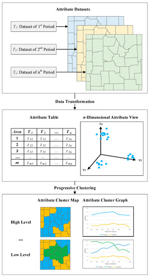
Figure 1.
The general framework of the Spatial-Temporal Indication of Crime’s Association (STICA).
Firstly, datasets for a specific attribute of a particular geographic phenomenon in different periods are created. Such datasets are typically area-based vectors or raster data. For consistency, all datasets should have an identical scale of measurement based on the same spatial units in equally temporal intervals, such as yearly neighborhood-based population, daily county-based temperature, and monthly state-based precipitation.
Secondly, via data transformation, values of the specific attribute are extracted from spatial units for all periodical datasets and integrated into a summarized attribute table. In this table, a row represents the record of a spatial unit, while a column denotes the attributive value in a temporal interval. If each column is defined as a dimension and each row is abstracted as a point, this tabular data can be considered as a set of points with n-dimensional coordinates, which are projected in an n-dimensional space. In this space, it is presumable that points are distributed under certain patterns, which can be potentially clustered into different classes. In summary, spatial units are categorized into different classes based on temporal likeness such that each class represents a group of spatial units with similar temporal patterns of the specific attribute. In terms of clustering methods, many clustering algorithms can be utilized, such as ISODATA and K-Means. In this step, more than one kind of clustering should be conducted.
Finally, based on the results from the progressive clustering, thematic mapping techniques can be utilized to distinguish each class of spatial units on the map. Simultaneously, a cluster graph is generated for each clustering result, which comprises straight lines connecting the specific value of each temporal dimension. For a cluster, these dimensional values not only represent the overall pattern to distinguish the cluster itself from the others, but also characterize the similar patterns of all spatial units in the cluster. To this end, these specific values are typically statistical measurements, such as the n-dimensional center of a cluster. Furthermore, via referencing the map and the graph side by side, researchers are able to comprehend not only how spatial units with similar temporal patterns are distributed in space but also how a category of spatial units varies in time. Based on these graphical indications of pertinent factors’ influence ranges in both space and time, further examination of the geographic phenomenon can be performed.
3.3. An Implementation of the STICA Approach
As noted in the above section, the STICA approach can be implemented with many specific algorithms. Here, this section presents one implementation. The methods and parameters for the three steps of the STICA framework are described in detail.
3.3.1. Dataset Representation
Kernel density estimation (KDE), a typical method for continuous surface smoothing, is selected to represent the crime data. It generates a smooth surface of crime risk over grids with uniform size based on the distribution of point-based crime incidents [10]. Of particular importance, the KDE result can to some extent reveal the spatial autocorrelation of crime events, which may be attributed to the movement patterns and the randomness of target-selection in a small area.
With respect to parameters, cell size and search radius have substantial impacts on the results and thus need specific consideration. On the one hand, since the geocoded accuracy of most burglary incidents in this study is about 20 m, the cell size was set to be 20 m for providing appropriate smoothness of burglary patterns. As such, there are 10,486 grid cells in the study area. On the other hand, previous research concluded that the spatial pattern of crime changes rapidly block by block [49], and near-repeat victimization presents similar spatial variations [50]; hence, given the environment of the study area, the search radius was set to 200 m to exhibit detailed variations of burglary patterns.
Furthermore, a series of KDE raster datasets with the same parameters were created on a monthly basis from January through December in 2010 using the ArcGIS 10.0. Then, the burglary densities for the 12 months in the 10486 grid cells were integrated into a matrix of 10,486 × 12, which is the input for the cluster analysis.
3.3.2. Progressive Clustering Analysis
Derived from the typical clustering algorithm, K-Means [51], this research presents a K-Median-Centers algorithm (Figure 2), and several key steps are articulated in subsections. Interested readers can contact the first author to obtain this program.
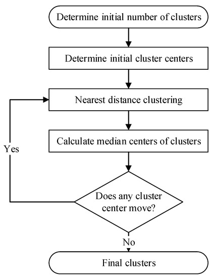
Figure 2.
A K-Median-Centers algorithm for the implementation of the STICA method in this study.
● Initial Cluster Centers
Over the entire study area, there are m cells with crime density z for n different periods. Derived from the expressions defined by Haining (2003) [52], datasets are described as:
where denotes the cell, n = 12, and m = 10,486. For k different clusters, their centers are denoted as:
where represents the center of the cluster, is the crime density at the dimension for the cluster. Specifically, the initial k cluster centers are determined according to the single pass algorithm utilized in IBM’s SPSS [51]. In this study, k is set as 4, 5, and 6 successively.
● Nearest Distance Clustering
The distance between a cell and a cluster in the n-dimensional space is defined by:
where represents the distance from cell to the cluster center and t denotes the dimension. For cell , its distance to each cluster is calculated, and it is categorized into the cluster with the shortest distance. Hence, the algorithm makes certain that a cell is classified into one and only one cluster, namely “divisibility.” In other words, for each cluster, suppose a spherical surface tightly envelops all its cell centers in the n-dimensional space, these surfaces will not overlap with each other.
● Median Centers of Clusters
In the K-Means clustering algorithm, the mean value is chosen to represent the cluster center; yet, it is easily influenced by outliers [53]. Therefore, it is replaced with a median center to denote the cluster center. It should be pointed out that the median center is different from the median value. Traditionally, among observations, the median value refers to either the middle value (the number of observations is odd) or the average of two middle values (the number of observations is even) in order. However, in this study, the concept of median-center is derived from that in a Euclidian plane; thus, for a cluster in the n-dimensional space, the summation of distances from its center to all its cells is minimized, so as to reflect the overall closeness of cells in the cluster and the tendency of cells towards the cluster center.
Recall that to calculate the median center on a Euclidean plane, an iterative approach is used with the mean center as the initial median center for efficiency [53]. Through iterations, the current median center becomes closer to both the previous median center and the true median center. If the distance between the current and previous median center is shorter than a threshold, the iterative process will be terminated and the current median center will be considered as the accurate median center; although theoretically, the true median center cannot be determined. Derived from the equations stated by Wong and Lee (2005), an iterative equation can be formulated for the cluster to calculate the dimension of its median center at iteration u:
where p is the number of cells in the cluster, r denotes the dimension, and the weight in the equations of Wong and Lee (2005) is set to 1 for simplicity [53]. With respect to termination, the threshold of the distance is 0.00001.
● Movement of Cluster Centers
For each cluster, its current center at the clustering process is differentiated from the previous center at the clustering process based on:
where denotes the center movement of the cluster at the clustering process compared to the clustering process. If the movements of all cluster centers are 0, all current cluster centers have not changed from the previous cluster centers and the cells in each cluster center remain the same. In this situation, all clusters are stable, and the clustering procedure is completed.
3.3.3. Thematic Mapping and Analysis
When the clustering procedure is completed, cells on the map are rendered variously based on the cluster they belong to, while the final median center of each cluster is plotted on the line graph. In this graph, the x-axis represents periods (i.e., dimensions), while the y-axis represents the value at each period. Using the median center instead of the mean value to construct the temporal graph is consistent with the algorithm, which characterizes the agglomerative intensity of cells in clusters.
3.4. Study Area and Data
The study area is the DP Peninsula located at the center of H City in southern China. The real names of both the peninsula and the city are abbreviated due to the confidentiality agreement with the police department of H city. The DP peninsula has been one of the major residential areas since 580 AD. In 2011, it covered about 4.2 km2 with a total population of almost 95,000, out of which permanent residents were nearly 63,000. Several shopping malls are located in the center of the DP peninsula, with a green park in the vicinity (Figure 3). Four types of residential communities, including traditional neighborhoods, Danwei communities, commercial communities, and urban villages, can be identified, while several industrial factories are scattered within the DP peninsula. Given the existence of diverse types of land use and residential community, it is a suitable city in miniature to conduct research on burglary [54].
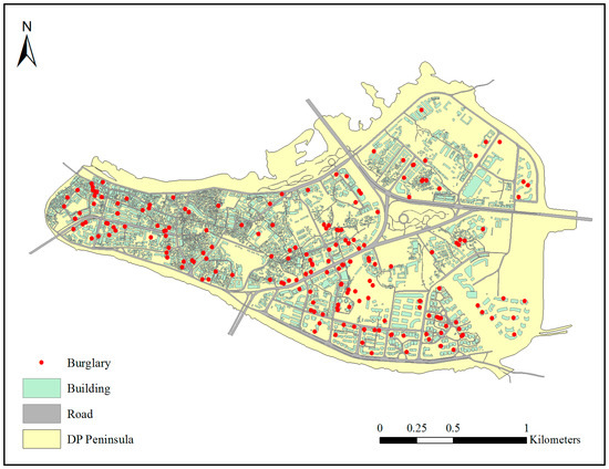
Figure 3.
The spatial distribution of burglary events in the study area in 2010.
The geographic data and burglary records were provided by the police department of the H city (Figure 3). Burglary incidents were recorded in a tabular format from January 1 to December 31 in 2010. They were generated from the 110 Emergency Response System, and the false alarms were removed based on the immediate investigation of the scene by a police officer. Due to the complicated address system in H city and the lack of precise address for some records, automatic geocoding is not applicable. Therefore, burglary incidents were geocoded manually, among which 200 incidents were successfully pinpointed on the DP Peninsula with a hit rate of 99%. In detail, 59% of burglary incidents were geocoded with a 20-m accuracy, while 88% of burglary incidents were located within 50 m from their presumably exact locations. In terms of the basic geographic data, it comprises a peninsula boundary, buildings, roads, and points of interest (POIs). Last but not least, on-the-spot investigations were conducted several times for understanding the environmental backcloth in 2011.
4. Results and Discussion
4.1. Estimating Monthly Kernel Density of Burglary
Following the conceptual framework, 12 KDE raster datasets on a monthly basis in 2010 were created, which illustrate that the spatial distribution of burglary has temporal variations (Figure 4). For instance, burglary hotspots displace monthly, while February has the fewest burglary hotspots in the year. Furthermore, the intensity of hotspots varies monthly, with 23.87 incidents/km2 as the lowest in January and 97.47 incidents/km2 as the highest in October. From these spatial burglary patterns, it is difficult to understand the temporal evolvement of the spatial crime pattern and to find meaningful influence factors of crime events. These raster datasets were applied to the conceptual framework to perform data transformation and cluster analysis, such that the areas with similar temporal characteristics of burglary can be identified and distinguished from one another.
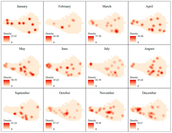
Figure 4.
Monthly kernel density estimation for the burglary in the DP peninsula in 2010 (Unit: Incidents per km2).
4.2. Discriminating Temporal Types and Spatial Hierarchies of Factors with the STICA Approach
As analyzed in the section of the theoretical basis for the STICA approach, an observed crime pattern is usually a result of the nested interactions of many factors, and these factors, either time-stable or time-varying, may exert influences on different spatial areas or act at diverse spatial scales. The first use of the STICA approach is to discriminate the type (time stable/varying) of factors that operate at different spatial scales. This can be achieved by comparing the multiple results from the STICA approach.
Two steps should always be followed when interpreting the multiple results of the STICA approach. The first step is to compare the crime zoning maps to identify the spatial areas that remain similar and those that show major changes among these zoning maps. For the spatial zones that remain similar, the temporal patterns of crime levels would also be similar. As such, the second step is to focus on the spatial areas that show major changes and compare the temporal crime patterns among different spatial zones, which are generated from the multiple results of the STICA approach. This would help to identify the type of main factors that operate at finer spatial scales. These would be demonstrated with the following empirical analysis.
In thematic mapping, four to six classes are recommended for the level of detailed visualization and reader’s comprehension [10,55]. Thus, to illustrate the feasibility of the STICA approach, this research classified the spatial areas into four, five, and six clusters, respectively, based on the temporal similarity of burglary density in each grid cell (Figure 5). As can be seen, both consistency and disparity exist among the STICA results with four, five, and six clusters (Figure 6, Table 1).
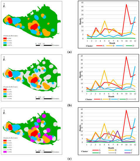
Figure 5.
The STICA results of burglary density. (a) four clusters; (b) five clusters; (c) six clusters.
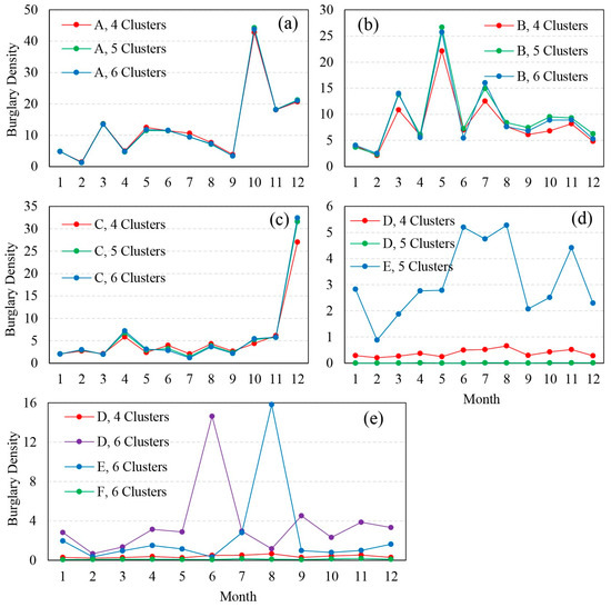
Figure 6.
Comparing temporal crime patterns for the STICA results with four, five, and six clusters. (a) Cluster As in the STICA results; (b) Cluster Bs in the STICA results; (c) Cluster Cs in the STICA results; (d) Cluster D in the four-cluster result and Cluster D & E in the five-cluster result; (e) Cluster D in the four-cluster result and Cluster D, E, & F in the six-cluster result.

Table 1.
Comparing the STICA results with four, five, and six clusters.
For the consistency, the Cluster As among the STICA results with four, five, and six clusters are similar in space (Figure 5) and have similar temporal patterns of burglaries (Figure 6a). Similar consistencies can also be found for the Cluster Bs (Figure 5 and Figure 6b) and Cluster Cs (Figure 5 and Figure 6c).
For the disparity, the spatial area of Cluster D in the four-cluster result (Figure 5a) is divided into areas of Cluster D and E in the five-cluster result (Figure 5b), while it is divided into areas of Cluster D, E, and F in the six-cluster result (Figure 5c).
On the one hand, for the five-cluster result, the burglary density in Cluster D is above that in Cluster E every month (Figure 6d). Similar characteristics can also be found when the burglary densities in Cluster D and E, as well as Cluster D and F, are compared in the six-cluster result (Figure 6e). This kind of yearlong difference indicates that the main factors that lead to the differences in burglary density between the above pairs of Clusters are stable in time.
On the other hand, for the six-cluster result, the burglary densities in Cluster E and F remain similar for most of the 12 months, while showing vast differences in June and August (Figure 6e). The burglary density in Cluster E has a peak in June, while the burglary density in Cluster F reaches the top in August. This kind of temporary difference indicates that the main factors that lead to the differences in burglary density between these two Clusters are time-varying.
In summary, by comparing multiple STICA results with different numbers of clusters, it is clear that the more clusters in the STICA result, the more discriminations in temporal fluctuations and spatial zones concurrently, and the more intrinsic potential factors indicated by these spatial-temporal differentiations. In other words, the STICA result with fewer clusters may reveal spatial-temporal patterns at coarse-grain levels and indicate the general influence factors in the occurrence of crime, while the STICA result with more clusters may uncover spatial-temporal patterns at fine-grain levels and signal moderate or minor influence factors in crime mechanisms.
4.3. Identifying and Understanding the Main Factors of Crime with the STICA Approach
This section illustrates two of the three uses for the STICA approach with a four-cluster STICA result as an example. One use of the STICA approach is to help identify time-stable factors of crime and relevant spatial zoning information which can be used to improve the performance of statistical models. The other use is to facilitate identifying time-varying factors of crime and understanding the complex interactions between these factors and the local/global environment.
To better illustrate the usability of STICA results in identifying the main influence factors of crime, the map in Figure 5a is redesigned with other geographic features overlaid and the graph embedded (Figure 7). It is argued that the overall trends and the monthly variations of crime in different zones are strong indications of the time-stable and time-varying factors of crime, which can be validated through on-the-spot investigations and other data sources.
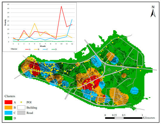
Figure 7.
The four-cluster result from the STICA approach and the geography in the DP peninsula.
4.3.1. Identifying and Understanding Time-Stable Factors of Crime with the STICA Approach
The STICA approach can be used to identify time-stable factors of crime by discriminating the yearlong differences among overall temporal trends of crime in different clusters. It can also provide the spatial zoning information for stable factors, which can be used in statistical modeling and improve the model performance.
The four-cluster result from the STICA approach conveys that the overall trends between clusters vary (Figure 7): Cluster D has the lowest burglary densities yearlong and its monthly average density is 0.38 incidents/km2; Cluster C has moderate burglary densities in most months and its monthly average is 5.48 incidents/km2; Cluster A and B have relatively high burglary densities for most months and their monthly averages are 8.19 incidents/km2 and 12.70 incidents/km2, respectively.
According to the routine activity approach, crime intensity is influenced by the frequency of convergence between offenders, targets, and the absence of capable guardians [22]. For burglary in this research, offenders are burglars, targets are residential and commercial units in the buildings, and capable guardians are mostly residents. Given that routine activities of residents are relatively similar throughout the DP Peninsula, while buildings vary spatially, it is further expected that the distribution of buildings and its interaction with offenders are non-temporary factors that contribute to the identified spatial-temporal patterns of burglary.
In terms of targets, on-the-spot investigations reveal that the buildings in Cluster A, B, and C are relatively dense and high-rise; hence, potential targets are plentiful. In contrast, Cluster D is mostly covered by green space and construction sites, while buildings are generally dispersed and low-rise; thus, potential targets are rare. The richness of potential targets determines that Cluster D has low burglary densities yearlong compared to the other clusters.
For the interactions between offenders and targets, burglars’ routine activities encompass activity nodes for residence, work, and leisure. Therefore, the distribution of activity nodes impacts the spatial pattern of burglar presence: Cluster A is the central business district in the DP Peninsula with large commercial areas (e.g., shopping malls) and the highest passenger flow; Cluster B has medium consumption places (e.g., markets) with a moderate passing flow; Cluster C is mostly residential with small retail spots (e.g., convenience stores) and a low passenger flow which mainly comprises local residents; and Cluster D has dispersed commercial places and residential dwellings, and thus, the passenger flow is the lowest. Given the variation of activity nodes and passenger flows in different zones, offenders’ inclination to commit burglary presumably decreases from Cluster A through D.
To quantitatively measure the effect of stable factors identified from the STICA, a linear regression model is constructed based on the geographic data obtained, among which only the data on buildings and POIs are currently available. In concert with the above analysis, it is hypothesized that burglary is generally influenced by the number of potential targets and offenders.
The dependent variable is the kernel density of burglaries for each cell in 2010. It is chosen due to two main reasons: First, in the real world, a burglary occurs in an area unit rather than a point with exact longitude and latitude; Second, the addresses of burglary events are geocoded with some locational uncertainties. The KDE is used to compensate for the above two endogenous limitations of the crime data.
A BuildingArea variable is created to serve as an approximate measure of the potential targets, since the number of commercial and residential units is not available. For each building, the building area is calculated as footprint area × the number of floors. Then, for each spatial cell, the amount of building area within it is calculated based on the geometrical relationships between the cells and buildings’ footprint.
A POI_KDE variable is created to serve as an approximate measure of the potential offenders. Based on the above theoretical analysis, an area with more POIs in its immediate and nearby environment usually attracts more people. As such, the POI_KDE value for each spatial cell is calculated with the KDE method. Here, the parameters remain the same as those in the implementation of the STICA approach.
Considering that there are four types of spatial zones identified in the STICA result, we also want to incorporate this spatial zoning information into this statistical modeling. The initial reason is that in terms of the urban environment, it is found that the inter-cluster variations are much larger than the intra-cluster variations according to our filed investigations. As such, these four types of spatial zones seem to represent different types of environmental settings for potential offenders’ behavior [56,57].
Here, the average value is used to represent the central characteristics for each cluster. For each cell, the values of BuildingArea and POI_KDE are replaced, respectively, with the average BuildingArea and average POI_KDE for the cluster it belongs to. That is, all cells in the same cluster would have the same value for either the building and the POI variable. Whether incorporating the spatial zoning information from the STICA result can improve the explanation power of the statistical model or not will be examined by comparing the performances of the following two models:
It should be noted that considering burglaries occur inside buildings, only the cells that intersect with the footprint of buildings were used for estimating the models.
The estimation results show that both models perform well. The Durbin–Watson statistics for both models are 1.976 and 1.960, suggesting that there is only a very slight autocorrelation in the regression residuals and both models are acceptable. For the first model, the variables of BuildingArea and POI_KDE do have a significant impact on burglary density, and they explain 20.2% of the variance for the dependent variable (Table 2).
Table 2.
Results of linear regressions for burglary density and stable factors.
More inspiringly, when the measurement of independent variables at the cell level is replaced with the measurement at the cluster level, a quite high adjusted R2 is yielded, increased from 0.202 to 0.595 (Table 2). In other words, the variation of burglary density at the cell level is indeed better explained by the variations of building area and POI density at the cluster level.
This seems surprising, but we do have a theoretical justification. When making behavioral decisions, an offender not only considers the surrounding environment within his vision but also the environment in a wider area. That is, the overall characteristics of a large environment would influence the behavior of offenders. As a result, offenders prefer to commit crimes in some type of urban environment rather than another type of environment. For example, it is found that the crime density in communities with many rural to urban migrants is much higher than that in communities with few migrants [26]. For a community or a large area, although among different sub-areas great variations of environmental features can be observed, it is usually perceived by an offender as a whole image, which can influence the way he reacts to the internal environment. When the offender is outside that type of area, they may react to the environment in a different way. As a result, the majority of the variation of crime can be explained by the environmental variations among different large areas rather than the environmental variations among different fine-grain areas.
The regression results not only verify the effects of stable factors, which are identified based on the STICA result, in a statistical way, but more importantly, they suggest that the exploratory approach presented in this research has great potential of facilitating statistical modeling by embedding stable factors at the cluster level. Specifically, this may become a new way regarding how to construct models. Traditional models, either one level or multiple levels, are developed based on grids or administrative areas, such as blocks, block groups, and tracts. However, the behavioral environment which is perceived as a whole by offenders may not coincide with these spatial units. In this regard, the spatial zoning information from the STICA results can be used to generate spatially contextual variables, which can be used to improve the performances of statistical models.
4.3.2. Identifying and Understanding Time-Varying Factors of Crime with the STICA Approach
The STICA approach can be used to identify time-varying factors of crime and corresponding mechanisms for their effects on crime through the graphical indication of their influence ranges in space and time. This can be achieved with the following three steps.
The first step is to identify the abnormal period in the temporal pattern of crime for each cluster. The second step is to seek answers to the question “what is the special factor of crime around the abnormal period?” The third step is to investigate “why does the effect of the identified factor appear only in some clusters and not in other clusters?”
To answer these questions, we need to synthesize theories and experiences, generate hypotheses, and verify with relevant data or previous research findings. If the hypotheses can be verified, then the time-varying factors can be accepted for further in-depth analyses. These are illustrated with the following empirical analysis.
Based on the boxplot of monthly burglary densities, three outliers can be identified from the four-cluster STICA result (Figure 8). For Cluster A, the burglary density increases dramatically in October; for Cluster B, an exceptionally high density of crime is observed in May; for Cluster C, a steep peak of burglary density is observed in December; for Cluster D, there is no outlier.
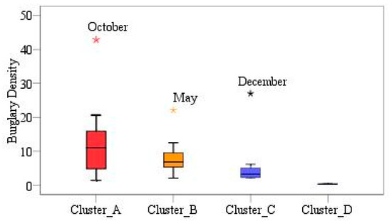
Figure 8.
The boxplot for monthly burglary densities in the four-cluster STICA result.
These three outliers raise the following questions that request explanation and verification:
Q1: Why is there a substantial increase of burglaries in October, and only in Cluster A?
Q2: Why is there a substantial increase of burglaries in May, and only in Cluster B?
Q3: Why is there a substantial increase of burglaries in December, and only in Cluster C?
For the first question, we first looked for the special factor that happens in October, examine how it is linked with the crime based on previous research findings, and verify the expected outcomes with finer-scale data. Thereafter, we put forward the hypothesis about why the effect of the special factor appears only in Cluster A and verify the hypothesis with relevant data.
Based on local knowledge, it is easy to discover that the most special factor in October is the National Day holiday, which lasts for 7 days from the 1st to 7th of the month, making it the longest statutory holiday in China. Previous research on crime and holidays show that offenders have similar activity habits to ordinary people and take a holiday as well [25,58]. As during a holiday people have a lot of free time to spend money for personal consumptions, it is expected that the National Day holiday contributes to the sharp increase of burglary in October in at least two ways: one is that during the holiday, offenders also spend a lot of money, leading to higher financial stress and stronger motivation to commit crimes for compensating their expenditure after the holiday; the other is that there are more attractive objects to be stolen by burglars after the National Day holiday, as people usually buy a lot of things during this long vacation. No matter the link between holiday and crime, it is expected that most of the increase of burglaries in October happens a few days after the National Day holiday. This expectation is validated by the temporal crime pattern at a finer scale. There is a significant increase of burglaries in middle October when compared to the other months in 2010 (Figure 9).
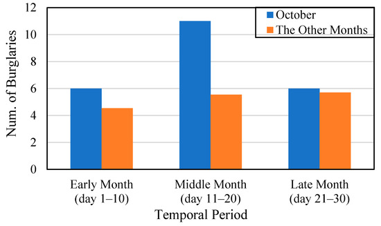
Figure 9.
The intra-month variations of burglary in October and the other months in 2010.
After the National Day holiday, potential offenders with stronger motivation would spend more effort and travel longer to seek opportunities for committing burglaries. Then, more potential offenders living outside of the DP peninsular would be expected to appear in the peninsula. As there are many constraints (e.g., capability, coupling) on individuals’ mobility, the chances of their appearances in the peninsula would not be evenly distributed in space. Considering that offenders organize their movement around activity nodes, it is expected that areas with more POIs would have more offenders and more burglaries. As such, among the four clusters, Cluster A is expected to have the most POIs. An examination of the spatial distribution of POIs (Figure 10) validates this hypothesis, thus adding credibility to our analysis.
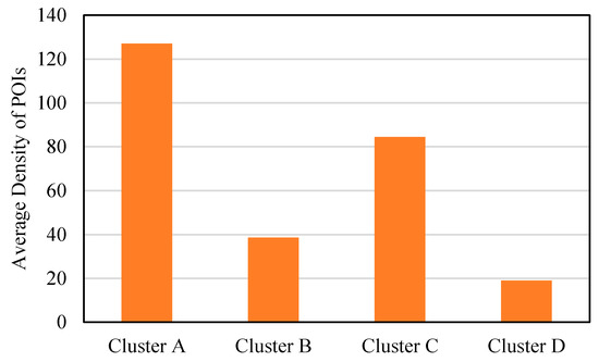
Figure 10.
The spatial distribution of POIs in the DP peninsula. Note: the density of POIs is obtained using the KDE with the parameters being the same as the other analyses. The average value is obtained based on all the grids (n = 10,486) in the peninsular.
For the second question, we first assume the special factor is the “plum rain” based on our local knowledge, verify the timing of its occurrence with historical weather data, and put forward the justification about the weather-crime relationship. Thereafter, we attribute the spatial locality of the weather’s effect to community features, present corresponding theoretical justification, and verify it with available data.
The “plum rain” is a local special weather phenomenon in southern China. It occurs in the first half of each year, while the specific month of its occurrence is not fixed. When the “plum rain” comes, there will be continuous rainfall that lasts for 1~2 weeks, and the air humidity will be so high that water vapor can condense on walls and floors as droplets. In such a humid environment, many indoor items, especially clothes, will get moldy. Based on our own life experience, many residents will choose to open windows for ventilation and drying clothes after the end of the “plum rain.” This could facilitate the entry of otherwise totally closed rooms and offer opportunities for potential burglars.
If our inference about the interactions between the “plum rain,” residents’ behaviors, and potential burglars is correct, then for explaining the substantial increase of burglaries in May 2010, the “plum rain” should have occurred mainly in April 2010. Thus, the next key task is to verify the timing of the “plum rain” in 2010 for the DP peninsula.
As this is a retrospective study, historical weather record data are used to confirm the timing of the “plum rain.” The historical weather record shows that during the first half of 2010, a substantial increase in the average daily rainfall happens in April and June (Figure 11). The daily average temperature in June was 26.7 °C, which is so high that the “plum rain” could not happen in such weather conditions. Thus, the timing of the “plum rain” in 2010 for the DP peninsula was mainly in April. This proves that our inference about the interactions between the “plum rain,” residents’ behaviors, and potential burglars is correct.
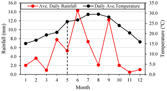
Figure 11.
The monthly variation of weather conditions in DP peninsula in 2010.
Bearing the “plum rain–residents’ behavior–potential burglars” interaction in mind, the next issue to investigate is why the weather’s effect on crime only applies in Cluster B. Based on the field observations on the local built environment, we attribute it to the uneven distribution of suitable targets in space, i.e., the characteristics of residential communities.
Residential buildings in Cluster B and Cluster C are commonly equipped with security meshes and other outside structures, which can be grabbed by offenders to facilitate their climbing. In Chinese cities, there is a large proportion of burglaries where the offender climbs up the building to enter a housing unit from the window. However, based on the physical appearance of buildings and the community environment, residents in Cluster B seem to have higher income and more valuable possessions than those in Cluster C. According to the rational choice theory [43], when there are plentiful opportunities for burglaries, cat burglars would be more prone to commit crimes in the wealthier Cluster B.
For the third question, it can be attributed to the increased offenders’ motivation, the uneven spatial distribution of POIs, and the differences in community organization levels. This conjecture can be partly proved by past findings and finer-scale temporal patterns of crime.
In China, many news reports and academic research have shown offenders’ motivation increases when the Spring Festival is coming; thus, the number of burglaries shows a general increase at the end of the year [59]. Additionally, if this conjecture is correct, we would expect the burglaries in December to show an increasing trend. An examination of the intra-month variations of burglary shows that compared with other months, the increasing trend of crime events is much more obvious (Figure 12). According to the above analysis, there are plentiful opportunities for burglaries in Cluster A, B, and C. As burglary increases at the end of the year, local police departments usually emphasize prevention and provide guidance to residents and communities. In this regard, the communities and residents in Cluster B are more willing to follow the official guidance, since the residential buildings are mostly high-end with effective management; hence, Cluster B does not show a dramatic increase of burglaries at the end of the year.
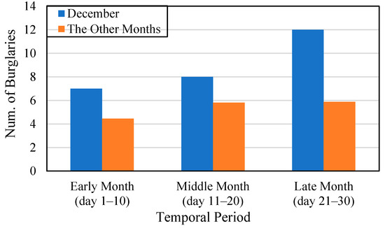
Figure 12.
The intra-month variations of burglary in December and the other months in 2010.
To summarize, the above analysis not only illustrates how to identify time-varying factors of crime with the graphical indication of temporal fluctuations of different clusters, but also illustrates how to understand the mechanisms of the spatially global factors in producing a spatially bounded crime-ridden zone with the spatial-temporal indications in the STICA result.
5. Conclusions
In place-based crime research, combining the spatial and temporal dimensions has been increasingly recognized as necessary and important. This paper presents a novel exploratory approach, Spatial-Temporal Indication of Crime Association (STICA).
The STICA approach is a general framework for identifying spatial-temporal crime patterns with progressive clustering. Distinguished from previous spatial-temporal crime analysis methods, this approach aims to progressively differentiate spaces with different temporal fluctuations of crime levels and can be implemented with various clustering techniques.
The STICA approach can be used to identify and understand the contributing factors of crime in at least three ways: (1) By comparing the multiple results from the STICA approach, the temporal types and spatial hierarchies of factors of crime can be discriminated. (2) The STICA approach can help to identify the time-stable factors of crime after discriminating the yearlong differences among the overall temporal trends of crime in different clusters and can provide the spatial zoning information of time-stale factors, which can be used to improve the performance of statistical models. (3) The STICA approach can facilitate identifying time-varying factors of crime and understanding the complex interactions between these factors and the environment by identifying the spatial-temporal localities of pertinent factors of crime.
The ability of the STICA approach in improving the understanding of crime mechanisms and modeling of crime patterns is demonstrated with an empirical case in China. A specific implementation of the STICA approach, which is based on the Kernel Density Estimation, K-median-centers clustering, and thematic mapping, is applied for the study of burglary in the DP peninsula, southern China.
In the illustration of interpreting the STICA results, four spatial zones with distinct temporal patterns are identified. On the one hand, the stable distribution of buildings and POIs throughout the year leads to the dissimilarities of overall trends between different spatial zones; on the other hand, specific national holiday and weather conditions contribute to monthly variations between these zones. More importantly, the statistical examination of stable factors shows that when incorporating spatial range information, the explanation power of stable factors can be greatly improved, while the comprehensive analysis of time-varying factors illustrates how these spatially global factors can produce a locally crime-ridden zone. By combining spatial and temporal aspects, the STICA approach can generate insight into possible crime mechanisms.
Although with inspiring primary results, the application of STICA still needs further examination. The next stage of this work is to examine the potential of using SITCA to gain a systematic understanding of crime and to examine the feasibility of incorporating STICA results into statistical modeling. As suggested in the above analysis, factors of different importance affecting crime may be indicated by STICA results with different numbers of clusters. A more systematic examination of STICA results with more clusters should be undertaken in future studies. However, challenges exist as unraveling the complex mechanisms of crime needs extensive theories, local knowledge, and multi-source data, especially when identifying time-varying factors. Additionally, as suggested in simple linear regressions of stable factors, the spatial range information in STICA results can facilitate better investigation through statistical modeling, when compared to the factors at the cell level. This primary finding highlights the importance of incorporating spatially contextual effects in understanding and modeling crime. Compared with other measurements (e.g., spatial lag), the degree of benefit that can be gained by measuring contextual effects with the STICA approach remains unclear. Solutions to these two issues will be of great value for better understanding and modeling crime patterns.
There exist limitations in this paper. For example, time-varying factors, such as the national holiday and the weather condition, have not been statistically examined at present, due to the difficulty in measuring and modeling temporal factors. This will be a focus of future research. Nonetheless, this study does not intend to validate the causations of crime; instead, this paper aims to delineate a new exploratory approach for identifying and visualizing spatial-temporal patterns of crime, which can facilitate deducing potential factors that trigger the patterns and understanding the underlying mechanisms. In this regard, with manageable techniques, explicable visualizations, and explainable outcomes, the STICA approach has demonstrated its feasibility in exploring contributing factors of crime and shows great potential for providing a new vision in place-based crime research.
Author Contributions
Conceptualization, Chao Jiang, Lin Liu and Xiaoxing Qin; Data curation, Chao Jiang and Kai Liu; Formal analysis, Chao Jiang, Lin Liu and Xiaoxing Qin; Funding acquisition, Chao Jiang, Lin Liu and Suhong Zhou; Investigation, Chao Jiang, Xiaoxing Qin and Kai Liu; Methodology, Chao Jiang, Xiaoxing Qin and Kai Liu; Project administration, Chao Jiang, Lin Liu, Suhong Zhou and Kai Liu; Resources, Kai Liu; Software, Chao Jiang and Xiaoxing Qin; Supervision, Lin Liu, Suhong Zhou and Kai Liu; Validation, Chao Jiang; Visualization, Chao Jiang and Xiaoxing Qin; Writing—original draft, Chao Jiang and Xiaoxing Qin; Writing—review and editing, Chao Jiang, Lin Liu, Suhong Zhou and Kai Liu. All authors have read and agreed to the published version of the manuscript.
Funding
This research was funded by the National Natural Science Foundation of China under a Young Scientists Fund (No. 42001159), a Key Program [No. 41531178], an Excellent Young Scholars Program [No. 41522104], and a General Program [No. 41171140]. It is also supported by a grant from the State Key Laboratory of Resources and Environmental Information System, China.
Data Availability Statement
Restrictions apply to the availability of these data. Data was obtained from the Public Security Bureau of H city and are available from the corresponding author with the permission of the Public Security Bureau of H city.
Acknowledgments
The authors would like to acknowledge the Public Security Bureau of H City for providing the crime and geographic data for academic research. The authors would like to thank Marcus Felson and John Bannister for their helpful suggestions on an earlier version of this paper when it was presented at the 4th International Conference on Crime Geography and Crime Analysis in Guangzhou, China. The authors also would like to thank the editor and three anonymous reviewers for their critical comments and constructive suggestions.
Conflicts of Interest
The authors declare no conflict of interest.
References
- The Oxford Handbook of Criminological Theory; Cullen, F.T., Wilcox, P., Eds.; Oxford University Press: New York, NY, USA, 2013. [Google Scholar]
- Shaw, C.R.; Mckay, H.D. Juvenile Delinquency and Urban Areas: A Study of Rates of Delinquency in Relation to Differential Characteristics of Local Communities in American Cities; University of Chicago Press: Chicago, IL, USA, 1942. [Google Scholar]
- Eck, J.E.; Weisburd, D. Crime and Place; Criminal Justice Press: Monsey, NY, USA, 1995. [Google Scholar]
- Guerry, A.M. Essai Sur la Statistique Morale de la France; Crochard: Paris, France, 1833. [Google Scholar]
- Harries, K.D. The Geography of Crime and Justice; McGraw-Hill: New York, NY, USA, 1974. [Google Scholar]
- Lebeau, J.L.; Leitner, M. Introduction: Progress in Research on the Geography of Crime. Prof. Geogr. 2011, 63, 161–173. [Google Scholar] [CrossRef]
- Liu, L.; Eck, J. Artificial Crime Analysis Systems: Using Computer Simulations and Geographic Information Systems; IGI Publishing: Hershey, NY, USA, 2008. [Google Scholar]
- Quetelet, M.A. A Treatise on Man and the Development of His Faculties; William and Robert Chambers: Edinburgh, UK, 1842. [Google Scholar]
- Weisburd, D.; Bernasco, W.; Bruinsma, G.J.N. Putting Crime in Its Place: Units of Analysis in Geographic Criminology; Springer: New York, NY, USA, 2009; pp. 1–254. [Google Scholar]
- Chainey, S.; Ratcliffe, J. GIS and Crime Mapping; John Wiley and Sons: Hoboken, NJ, USA, 2005. [Google Scholar]
- Sherman, L.W.; Gartin, P.R.; Buerger, M.E. Hot Spots of Predatory Crime: Routine Activities and the Criminology of Place. Criminology 1989, 27, 27–56. [Google Scholar] [CrossRef]
- Ratcliffe, J.H. The Hotspot Matrix: A Framework for the Spatio-Temporal Targeting of Crime Reduction. Police Pract. Res. 2004, 5, 5–23. [Google Scholar] [CrossRef]
- Sherman, L.W.; Weisburd, D. General deterrent effects of police patrol in crime “hot spots”: A randomized, controlled trial. Justice Q. 1995, 12, 625–648. [Google Scholar] [CrossRef]
- He, L.; Páez, A.; Liu, D. Persistence of Crime Hot Spots: An Ordered Probit Analysis. Geogr. Anal. 2016, 49, 3–22. [Google Scholar] [CrossRef]
- Weisburd, D.; Telep, C.W.; Braga, A.A. The Importance of Place in Policing—Empirical Evidence and Policy Recommendations; The Swedish Crime Prevention Council: Stockholm, Sweden, 2010. [Google Scholar]
- Townsley, M. Visualising space time patterns in crime: The hotspot plot. Crime Patterns Anal. 2008, 1, 61–74. [Google Scholar]
- Nagin, D.S. Analyzing Developmental Trajectories: A Semiparametric, Group-Based Approach. Psychol. Methods 1999, 4, 139–157. [Google Scholar] [CrossRef]
- Weisburd, D. Place-Based Policing. Police Found. 2008, 9, 1–16. [Google Scholar]
- Johnson, S.D.; Bowers, K.J. The Stability of Space-Time Clusters of Burglary. Br. J. Criminol. 2004, 44, 55–65. [Google Scholar] [CrossRef]
- Johnson, S.D.; Lab, S.P.; Bowers, K.J. Stable and Fluid Hotspots of Crime: Differentiation and Identification. Built Environ. 2008, 34, 32–45. [Google Scholar] [CrossRef]
- Mohler, G.O.; Short, M.B.; Brantingham, P.J. The Concentration-Dynamics Tradeoff in Crime Hot Spotting. In Unraveling the Crime-Place Connection; Weisburd, D., Eck, J.E., Eds.; Routledge: New York, NY, USA, 2017; pp. 19–39. [Google Scholar]
- Cohen, L.E.; Felson, M. Social Change and Crime Rate Trends: A Routine Activity Approach. Am. Sociol. Rev. 1979, 44, 588. [Google Scholar] [CrossRef]
- Eck, J.E. Examining routine activity theory: A review of two books. Justice Q. 1995, 12, 783–797. [Google Scholar] [CrossRef]
- Brantingham, P.B. Nodes, Paths, and Edges: Considerations on the Complexity of Crime and the Physical Environment (1993). Class. Environ. Criminol. 2010, 13, 289–326. [Google Scholar] [CrossRef]
- Cohn, E.G.; Rotton, J. Even criminals take a holiday: Instrumental and expressive crimes on major and minor holidays. J. Crim. Justice 2003, 31, 351–360. [Google Scholar] [CrossRef]
- Du, F.; Liu, L.; Jiang, C.; Long, D.; Lan, M. Discerning the Effects of Rural to Urban Migrants on Burglaries in ZG City with Structural Equation Modeling. Sustainability 2019, 11, 561. [Google Scholar] [CrossRef]
- Anselin, L.; Cohen, J.; Cook, D.; Gorr, W.; Tita, G. Spatial Analyses of Crime. Measurement and Analysis of Crime and Justice. Rev. Crim. Justice 2000, 4, 213–262. [Google Scholar]
- He, L.; Páez, A.; Jiao, J.; An, P.; Lu, C.; Mao, W.; Long, D. Ambient Population and Larceny-Theft: A Spatial Analysis Using Mobile Phone Data. ISPRS Int. J. Geo-Inf. 2020, 9, 342. [Google Scholar] [CrossRef]
- Grubesic, T.H.; Mack, E.A. Spatio-Temporal Interaction of Urban Crime. J. Quant. Criminol. 2008, 24, 285–306. [Google Scholar] [CrossRef]
- Brunsdon, C.; Corcoran, J.; Higgs, G. Visualising space and time in crime patterns: A comparison of methods. Comput. Environ. Urban Syst. 2007, 31, 52–75. [Google Scholar] [CrossRef]
- Lersch, K.M.; Hart, T.C. Space, Time, and Crime; Carolina Academic Press: Durham, NC, USA, 2011. [Google Scholar]
- Butt, U.M.; Letchmunan, S.; Hassan, F.H.; Ali, M.; Baqir, A.; Sherazi, H.H.R. Spatio-Temporal Crime HotSpot Detection and Prediction: A Systematic Liter-ature Review. IEEE Access 2020, 8, 166553–166574. [Google Scholar] [CrossRef]
- Leong, K.; Sung, A. A review of spatio-temporal pattern analysis approaches on crime analysis. Int. e-J. Crim. Sci. 2015, 9, 1. [Google Scholar]
- Dorling, D. Stretching Space and Splicing Time: From Cartographic Animation to Interactive Visualization. Cartogr. Geogr. Inf. Syst. 1992, 19, 215–227. [Google Scholar] [CrossRef]
- Brunsdon, C. The comap: Exploring spatial pattern via conditional distributions. Comput. Environ. Urban Syst. 2001, 25, 53–68. [Google Scholar] [CrossRef]
- Rey, S.J.; Mack, E.A.; Koschinsky, J. Exploratory Space-Time Analysis of Burglary Patterns. J. Quant. Criminol. 2012, 28, 509–531. [Google Scholar] [CrossRef]
- Short, M.B.; Brantingham, P.J.; Bertozzi, A.L.; Tita, G.E. Dissipation and displacement of hotspots in reaction-diffusion models of crime. Proc. Natl. Acad. Sci. USA 2010, 107, 3961–3965. [Google Scholar] [CrossRef] [PubMed]
- Berestycki, H.; Nadal, J.P. Self-organised critical hot spots of criminal activity. Eur. J. Appl. Math. 2010, 21, 371–399. [Google Scholar] [CrossRef]
- Nakaya, T.; Yano, K. Visualising Crime Clusters in a Space-time Cube: An Exploratory Data-analysis Approach Using Space-time Kernel Density Estimation and Scan Statistics. Trans. GIS 2010, 14, 223–239. [Google Scholar] [CrossRef]
- Townsley, M.; Homel, R.; Chaseling, J. Infectious Burglaries. A Test of the Near Repeat Hypothesis. Br. J. Criminol. 2003, 43, 615–633. [Google Scholar] [CrossRef]
- He, Z.; Tao, L.; Xie, Z.; Xu, C. Discovering spatial interaction patterns of near repeat crime by spatial association rules mining. Sci. Rep. 2020, 10, 1–11. [Google Scholar] [CrossRef]
- He, Z.; Deng, M.; Cai, J.; Xie, Z.; Guan, Q.; Yang, C. Mining spatiotemporal association patterns from complex geographic phenomena. Int. J. Geogr. Inf. Sci. 2019, 34, 1162–1187. [Google Scholar] [CrossRef]
- Clarke, R.V.; Cornish, D.B. Modeling Offenders’ Decisions: A Framework for Research and Policy. Crime Justice 1985, 6, 147–185. [Google Scholar] [CrossRef]
- Brantingham, P.L.; Brantingham, P.J. Environment, Routine, and Situation: Toward a Pattern Theory of Crime. In From Routine Activity and Rational Choice: Advances in Criminological Theory; Clarke, R.V., Felson, M., Eds.; Transaction Publishers: Piscataway, NJ, USA, 1993; pp. 259–294. [Google Scholar]
- Ratcliffe, J.H.A. Temporal Constraint Theory to Explain Opportunity-Based Spatial Offending Patterns. J. Res. Crime Delinq. 2006, 43, 261–291. [Google Scholar] [CrossRef]
- Clarke, R.V. Opportunity makes the thief. Really? And so what? Crime Sci. 2012, 1, 1–9. [Google Scholar] [CrossRef]
- Hägerstrand, T. What about people in Regional Science? Pap. Reg. Sci. 1970, 24, 6–21. [Google Scholar] [CrossRef]
- Lin, C. The Impact of Football Games on Crime: A Routine Activity Approach. Ph.D. Thesis, University of Maryland, College Park, MD, USA, 2007. [Google Scholar]
- Groff, E.R.; Weisburd, D.; Yang, S.M. Is it important to examine crime trends at a local “micro” level?: A longitudinal analysis of street to street variability in crime trajectories. J. Quant. Criminol. 2010, 26, 7–32. [Google Scholar] [CrossRef]
- Johnson, S.D.; Bernasco, W.; Bowers, K.J.; Elffers, H.; Ratcliffe, J.; Rengert, G.; Townsley, M. Space-Time Patterns of Risk: A Cross National Assessment of Residential Burglary Victimization. J. Quant. Criminol. 2007, 23, 201–219. [Google Scholar] [CrossRef]
- IBM. IBM SPSS Statistics 20 Algorithms; IBM: Armonk, NY, USA, 2011. [Google Scholar]
- Haining, R. Spatial Data Analysis: Theory and Practice; Cambridge University Press: Cambridge, UK, 2003. [Google Scholar]
- Wong, D.W.S.; Lee, J. Statistical Analysis of Geographic Information with ArcView GIS and ArcGIS; Wiley: Hoboken, NJ, USA, 2005. [Google Scholar]
- Liu, L.; Jiang, C.; Zhou, S.; Liu, K.; Du, F. Impact of public bus system on spatial burglary patterns in a Chinese urban context. Appl. Geogr. 2017, 89, 142–149. [Google Scholar] [CrossRef]
- Dent, B.D.; Torguson, J.S.; Holder, T.W. Cartography: Thematic Map Design; McGraw-Hill Higher Education: New York, NY, USA, 2008. [Google Scholar]
- Brantingham, P.L.; Brantingham, P.J. Burglar mobility and crime prevention planning. In Coping with Burglary: Research Perspectives on Policy; Clarke, R., Hope, T., Eds.; Kluwer-Nijhoff Publishing: Hingham, MA, USA, 1984. [Google Scholar]
- Barker, R.G. Ecological Psychology: Concepts and Methods for Studying the Environment of Human Behavior; Stanford University Press: Stanford, CA, USA, 1968. [Google Scholar]
- Zimring, F.E.; Ceretti, A.; Broli, L. Crime Takes a Holiday in Milan. Crime Delinq. 1996, 42, 269–278. [Google Scholar] [CrossRef]
- Wang, Z. Temporal-Spatial Hot Spot Analysis on Crime Cases Based on Scan Statistics Methodologies in Shanghai. Ph.D. Thesis, East China Normal University, Shanghai, China, 2013. [Google Scholar]


Publisher’s Note: MDPI stays neutral with regard to jurisdictional claims in published maps and institutional affiliations. |
© 2021 by the authors. Licensee MDPI, Basel, Switzerland. This article is an open access article distributed under the terms and conditions of the Creative Commons Attribution (CC BY) license (http://creativecommons.org/licenses/by/4.0/).