1. Introduction
A Discrete Global Grid (DGG) is a spatial structure based on a spherical (or ellipsoidal) surface that can be subdivided infinitely without changing shape and simulates the shape of the Earth’s surface [
1,
2]. The various resolution grids form a hierarchy with a high degree of regularity and strict transformation relationships among the DGGs [
3]. This provides a unified expression mode that can fuse unevenly distributed geographical phenomena at different scales [
4,
5]. DGGs have been widely used in large-scale spatial data management, decision making, and simulation analysis. For example, they have been used in the spatial data organization, indexing, analysis, and visualization [
6,
7,
8,
9]; global environmental and soil monitoring models [
10,
11]; atmospheric numerical simulations and visualizations [
12]; ocean numerical simulations and visualizations [
13]; place names management or gazetteers [
14]; big Earth data observations [
12,
15]; modeling of offset regions around the locations of Internet of Things (IoT) devices [
16]; cartographic generalization and pattern recognition for choropleth map-making [
17]; the Unmanned Aerial Vehicle (UAV) data integration and sharing [
18]; the Modifiable Areal Unit Problem (MAUP) [
19]; especially in digital Earth [
5,
16,
20,
21,
22], and so on.
Most of the DGGs are generated from five regular polyhedrons (tetrahedron, hexahedron, octahedron, dodecahedron, and icosahedron) to limit the effects of non-uniformity of the latitudinal and longitudinal grid and the singularity of the poles. In the first level, the cells of a DGG are uniform, but their geometric deformation increases with the subdivision level [
23]. Because of the non-uniformity of DGGs, there is uncertainty in the spatial data expression, analysis, or decision-making, which greatly restricts their applications to fields with low accuracy such as data indexing, meteorological, and environmental monitoring [
24]. However, large-scale and high-precision applications and comprehensive spatial analyses of the DGGs are not available [
25]. Therefore, the application of reliable and credible DGGs needs a quality evaluation system or error control model of the deformation of the spherical (or ellipsoidal) grids [
26,
27]. From the 1990s, many researchers have discussed the geometric deformation and quality evaluation of DGGs. In the early stages, Goodchild (1994) proposed the first set of quality evaluation criteria of DGGs. These were supplemented and modified by other researchers, and an updated and integrated 14-terms list was provided by Kimerling [
28], which was called the Goodchild Criteria (
Appendix A). The Goodchild Criteria became a standard for quality evaluation of DGGs, and an ideal description of DGGs. These criteria include domain, area, topology, shape, compactness, edge, midpoints, hierarchy, uniqueness, location, center-point spacing, structure, grids transformation, and spatial resolution. Clarke [
29] conducted a qualitative evaluation and analysis of the Goodchild Criteria from 10 terms or aspects, including, for example, universality, authority, succinctness, hierarchy, uniqueness, etc. Clarke also pointed out that the Goodchild Criteria concerned primarily with the geometric features rather than the topological features of the DGG.
Recently, researchers have been interested in the quantitative indicators of the Goodchild Criteria, constructing new quantitative indicators to evaluate and analyze the geometric deformation of DGG [
30]. Heikes and Randall picked the midpoints from the Goodchild Criteria (no. 7 in
Appendix A) and constructed a method to measure the distance between the midpoint of the arc connecting two adjacent cell centers and the midpoint of the edge between the two cells [
31]. They improved an atmospheric process model based on the midpoints indicator and concluded that the midpoints were an extension of the concept of DGGs. White made choices of indicators of area and shape from the Goodchild Criteria [
32]. The surface area of the cell and its perimeter were measured to calculate the normalized area and the normalized compactness, respectively, to evaluate the deformation of DGGs. Kimerling considered that area, compactness, and center-points spacing (no. 2, 5, and 11 in
Appendix A) were the most important indicators to evaluate the deformation of a DGG [
28]. The three indicators were measured by cell surface area, zone spherical compactness (ZSC), and the intrinsic distance of the center points of adjacent cells, respectively. These indicators were compared to represent the deformation features of the DGG. Zhao selected indicators of area and edge (no. 2 and 6 in
Appendix A) to assess a variation of the Quaternary Triangular Mesh (QTM) [
33]. The cell area and its length were measured as observation data of the two indicators above, which uncovered their convergence and spatial distribution features [
34]. Ben chose the edge indicator (no. 6 in
Appendix A) and compared the advantages and disadvantages of three equal-area spherical hexagonal grid models using observation data of the cell edge length, which would be used to calculate its perimeter, as well as features of convergence and spatial distribution of the edge indicator [
35]. Gregory compared the midpoints and center-points spacing (no. 7 and 11 in
Appendix A) using the coefficient of variation to describe their performance and relative merits [
36]. Tong selected the indicators of area (no. 2 in
Appendix A), edge (no. 6 in
Appendix A), cell center radius (distance between the center point of a cell and its edge point, not part of the Goodchild Criteria), and cell center angle (angle between the center point of the cell and the two ends of its edge, also not part of the Goodchild Criteria) [
37]. Zhang chose indicators of area (no. 2 in
Appendix A), compactness (no. 5 in
Appendix A), and internal angle (fuzzy similarity of internal cell angle, not part of the Goodchild Criteria) to assess their convergence and spatial distribution of the DGG [
38]. Similarly, Sun and Zhou chose area and its measurement method to study the spatial distribution of the DGG [
39]. Recently, area (no. 2 in
Appendix A) and its measurement were selected by Zhao, and its features of convergence and spatial distribution for QTM based on “latitude loop” were revealed [
40].
In summary, most of the indicators selected for the deformation evaluation of the DGG model are from the Goodchild Criteria. The evaluations are mainly based on single or several indicators separately. A comprehensive evaluation is still missing because the Goodchild criteria include contradictory and repetitive evaluation indicators, and thus no DGG model can meet all the criteria at the same time [
28]. Therefore, if all Goodchild Criteria were directly used to evaluate a DGG model’s quality, the information among different evaluation indicators would overlap and may lead to inaccurate or unreliable results.
In this paper, we will:
eliminate contradictory and duplicate information,
calculate and analyze the correlations among the Goodchild Criteria, and
reconstruct a comprehensive and reliable quality evaluation system of DGGs with independent indicators.
The rest of this paper is organized as follows.
Section 2 describes the proposed method, classifies the Goodchild Criteria into qualitative and quantitative evaluation indicators, and establishes the correlation model of the quantitative evaluation indicator.
Section 3 presents the test and verification of the research method. Taking the QTM model as an example, it tests the research method for one level and applies it to other subdivision levels for comparison and verification. In
Section 4, by analysis and integration of qualitative and quantitative indicators, the quality evaluation indicator system of the DGG is reconstructed. Finally, the paper summarizes the research results and contributions.
2. Methods
The Goodchild Criteria can be sorted into two categories: qualitative evaluation indicators and quantitative evaluation indicators. The former describes categorical variables that can be distinguished with a “yes or no” or “with or without”, and are no. 1 (domain), no. 3 (topology), no. 8 (hierarchy), no. 9 (uniqueness), no. 10 (location accuracy), no. 13 (grids transformation), and no. 14 (spatial resolution). The latter can be calculated quantitatively, i.e., no. 2 (area), no. 4 (shape), no. 5 (compactness), no. 6 (edge), no. 7 (midpoints), no. 11 (center-point spacing), and no. 12 (structure).
The correlations among the quantitative indicators were calculated by factor analysis. Indicators with incompatible and overlapping information were eliminated or merged. The internal dependency relationship was then obtained by naming and interpreting the indicator with expert knowledge, and independent factors were extracted to construct a revised evaluation indicator system. The process is shown in
Figure 1, and the steps are as follows:
The Goodchild Criteria Sorting. The Goodchild Criteria are assigned into two groups: qualitative evaluation indicators and quantitative evaluation indicators. We classify the indicators according to their nature or properties.
Quantitative Evaluation Indicators. These indicators can be measured and calculated by the formulae of
Section 2.1. As a result, indicators correlation matrix is created. With professional knowledge, common factors and their loadings will be extracted from the matrix.
Elimination and Merging of Indicator Correlation. Qualitative Indicators will be analyzed in
Section 4. After quantitative indicators calculation and qualitative indicators analysis, we eliminate and merge the relevant indicators. This process needs to be combined with specific applications.
Independent Evaluation Indicator Set. The independent indicators set is formed here. From the set, we select single- or multi-indicator to evaluate DGGs.
Comprehensive Evaluation Model for DGGS. Considering the indicators set, weight of indicators, and other factors, we will construct a comprehensive evaluation model for DGGs.
2.1. Measurement of Quantitative Indicators
The measurement methods of the quantitative indicators were designed first. The coordinates of
vertices of the grid cell are denoted as
. In spherical coordinates, a point is represented as
in radians (see
Figure 2), where
is latitude (
) and
is longitude (
). Conversion from the coordinates
to the Cartesian coordinates
of any point on the Earth were calculated as Formula (1) [
41]
where,
is the radius of the Earth. The values of
and
, if needed, can be calculated from the inverse of Formula (1). Because the domain of
is
, the value of
depends on not only
but also where
and
are.
Area of the actual region represented by a grid cell is denoted by . The calculation was based on the shape of the DGG and the properties of the grid cell edge.
Shape of the grid cell was measured by the Landscape Shape Index. This term comes from landscape ecology and is an indicator that expresses the shape characteristics of the patches in the whole landscape [
42]. The Landscape Shape Index represents the degree of deviation between the shape of patches and a regular geometric figure or polygon whose area is equal to the patches, such as a square or a circle, and represents the shape complexity of the grid cells instead of patches. The formula of the Landscape Shape Index
[
42] is:
where,
is the cell area and
is its perimeter. Let
be 1.0, and
can be calculated. If the regular polygon is a spherical triangle, the triangular landscape shape is used and the cell is compared with a regular spherical triangle of the same area. Given an equilateral triangle with its side length
, its area
is
, and its perimeter
is
. And
calculated by Formula (2) is
. Similarly, if the regular polygon is a square with its length
(see
Figure 3), the cell is compared with a regular spherical quadrilateral of the same area and
, and if the regular shape is a circle, the cell is compared with a spherical circle with the same area and
.
Compactness of the grid cell is the ratio of the surface area of the cell to its circumference. In this paper, compactness
was calculated as the Zone Standardized Compactness (ZSC) [
28]. ZSC is given by zone_perimeter/cell_perimeter. Let the surface area of a spherical zone be equal to the zone surface area (see
Figure 4), so that the latitude of the bounding parallel is obtained. The perimeter of spherical zone which is the circumference of the bounding parallel can be computed. Substituting and combing equations, we compute
from:
where,
is the cell area,
is its perimeter, and
is the radius of the Earth.
Edge, the length of the cell side, is denoted by
. Depending on the nature of the grid, the cell sides may be arcs of great circles, small arcs, or even arbitrary curves. If the boundary of a cell is an arc of a great circle, the actual length of the edge is calculated according to Formula (4); if it is a small or a parallel arc, Formula (5) is used. The two endpoints of the cell side are denoted as
and
(see
Figure 5). If the edge is an arc of a great circle, the length (denoted by
) is the intrinsic distance [
43] between its two endpoints.
where,
is the radius of the Earth, and
The range of
varies according to the scale or subdivision level of the DGG. If the edge is a small arc or a parallel arc, the length (denoted by
) is:
where,
is the radius of the Earth, and
Identically, the range of varies according to the scale or subdivision level of the DGG.
Midpoints are the center-point of a cell boundary [
36] and the center-point of the edge between the two cells (no. 7 of Goodchild Criteria). The two cells involved in the indicator must be two adjacent cells, i.e., the faces where the two cells are located intersect along the side; otherwise, the indicator is invalid. This indicator calculates the geodesic distance between the two midpoints, i.e., the intrinsic distance or great circle distance between the two midpoints, denoted by
, and the calculation formula is shown in Formula (4).
Center-point Spacing, the distance between the center points of adjacent grid cells, includes the distance between cells adjacent by edges and the distance between cells adjacent by angles and is represented by the symbols
and
, respectively. The measurement of the adjacent distance indicator is the length of the geodesic between the reference points of adjacent cells, i.e., the intrinsic distance or great circle distance between two reference points. The calculation method is shown in Formula (4). In this paper, the center point of the cell is taken as the reference point, and the center point is taken as the spherical mean of the cell [
41], so the distance between adjacent cells is the length of the geodesic between the sphere medians of two adjacent cells.
The spherical mean is a point on the sphere surface, and its location is calculated by Formula (6) [
41]. Let the spherical mean of a cell be
, and the vertexes coordinates of the cell be
.
is shown in Formula (6):
where,
.
Structure, whether it is regular or arbitrary, is an important attribute of the grid model, and it is the basis for obtaining geocoding and run efficient algorithms of the grid [
28]. Because regularity is not easy to quantify, the irregularity indicator used to measure patches in landscape ecology is introduced, i.e., the fractal dimension
[
44]. In normal circumstances, there would be
, and
. For the sake of simplicity, let the parameter
be 0.0. Therefore, the fractal dimension
is:
where,
is the cell area and
is the perimeter of the cell.
2.2. Correlation and Evaluation System of Indicators
We calculated the correlation of the evaluation indicators with observation data. In any layer of the DGG, the number of grid cells is and the number of evaluation indicators is . According to the evaluation indicator calculation formula, groups of observation data are obtained, and each group of observation data is denoted by .
Standardization of the original observation data
. Due to the different nature of the evaluation indicators, the magnitude or dimension of the obtained observation data is different. Therefore, to ensure the reliability of the results, we standardized the original observation data to eliminate the influence of the order of magnitude or dimension. The standardized observed value of the indicator [
45] is calculated as:
Correlation matrix
. For the standardized observation data, we calculated the correlation matrix [
45] among the indicator variables
:
Eigenvalue
and the cumulative contribution rate
of the correlation matrix
. The eigenvalue
of matrix
can be obtained by matrix transformation. According to the cumulative contribution rate, the first
(
) principal components were used to express the information of the model. The cumulative contribution rate [
45] of the first
principal components was calculated as:
Factor loading matrix
. In the cumulative contribution rate
of the eigenvalues, if the cumulative contribution of the first
principal components reaches 85%, i.e.,
≥ 85%, it indicates that the first
principal components contain most (i.e., 85%) of the information of all the measurement indicators. Taking the first
principal components as independent factors, we built the factor loading matrix
, and the correlation matrix
is simplified to Formula (11) [
45]. Clearly, a factor loading
can be obtained by
divided by the square root of the corresponding eigenvalue (i.e.,
):
where,
and
. Therefore, factor loading matrix
is obtained.
Indicator analysis and classification. The quantitative indicators were classified according to their correlation. Each indicator was assigned to common factors ( categories) based on their absolute value in the factor loading matrix . The maximum variance method was used to rotate the factor loading matrix so that the matrix had a compact structure and the common factors more clearly expressed the information of the relevant indicators. The common factor loading coefficient may be represented by the factor weight assigned based on expert knowledge.
Restructuring of the evaluation indicator system. The contradictory and repetitive components of the evaluation indicators were eliminated using expert knowledge and the factor naming and interpretation, and merged. In this way, the number of indicators was decreased to form a new independent and comprehensive evaluation system that served the applications of DGGs.
4. Analysis and Discussion
4.1. Qualitative Analysis
The qualitative indicators of the Goodchild Criteria include no. 1, 3, 8, 9, 10, 13, and 14. The details are as follows:
No. 1 is summarized as a spatial domain and indicates whether the grid coverage is the Globe. This indicator does not only clarify the basic research object but also defines the scope of the grid model. This study retains this indicator.
No. 3 is summarized as topology and indicates whether the grid maintains topological consistency. This indicator only requires the relative positional relationship between objects to remain unchanged, but not their shape and size, i.e., the relative positional relationship and number of points, lines, and surfaces remain unchanged. If the shape of the grid cell does not change, then the relationship and number of cell vertices and cell edges must be the same, i.e., the topological relationship among points, lines, and surfaces does not change. If the topological relationship is unchanged, the consistency of shape and size cannot be guaranteed. Therefore, a shape that remains unchanged is a sufficient and unnecessary condition for the topology to remain unchanged. This means that indicator 4 is a sufficient and unnecessary condition of indicator 3. Indicator 3 can be derived from indicator 4. This study merges indicator 3 with 4.
No. 8 is summarized as hierarchy, indicating whether the grid is hierarchical. The hierarchy indicator has two meanings. First, the indicator requires the grid to have a hierarchical relationship, i.e., the grid can be subdivided into different levels. Secondly, the hierarchy requires that the bottom level or sub-grid can form a top-level or the parent grid, i.e., the combination of sub-grid cells overlaps with the parent grid. The hierarchy determines that the grid can be subdivided into more detailed grid cells. This article retains this indicator.
No. 9 is summarized as uniqueness and indicates whether the reference point of the cell is unique. This indicator is universal for all DGGs. The reference point constitutes a point grid, which is located on the surface of the cell and can directly participate in calculations. Whether the reference point is unique is related to the value of the reference point.
No. 10 is summarized as cell positioning and indicates whether the reference point is closest to the center of the cell. The center of the cell is unique. Once the center point is taken as the reference point, the reference point of the grid is unique. If another point is selected as the reference point, the reference point must not be the point closest to the center of the grid cell. Therefore, indicator 10 is a sufficient and unnecessary condition for indicator 9. Accordingly, this article takes the central point as the reference point and merges indicator 9 with 10. The DGG model is a surface model. According to its definition, the Spherical Mean is the center point of the spherical polygon [
41], which is also the point of the spherical polygon on the sphere. The Spherical Mean of the sphere as a reference point satisfies both indicator 9 and 10. Therefore, this article takes the Spherical Mean of the cell as the center (i.e., reference) point.
No. 13 is summarized as transformation, i.e., whether the coordinate of the grid can be simply transformed into a longitude–latitude grid. This indicator requires a simple geometric relationship between the grid model cell and the square-like longitude–latitude grid cell. Generally, if the grid model conforms to specific subdivision rules, there must be a geometric relationship between the grid model and the latitude–longitude grid model. Particularly, it is obvious that if the edges of the grid cell and the graticule have the same properties, the transformation must be easy. This indicator belongs to the application category of the grid model, i.e., the grid model has the function of interoperating with the longitude–latitude grid. This indicator is an extension of the concept of the grid model, so this article retains this indicator.
No. 14 is summarized as spatial resolution, i.e., whether the grid has an infinite spatial resolution. This indicator requires that the grid can be infinitely subdivided in the current space. Indicator 8 requires that the grid can be subdivided spatially and does not limit the degree of subdivision. That means that indicator 8 can achieve the requirement of indicator 14 infinite subdivision in space. Under the premise of indicator 1, indicator 8 is a sufficient condition for indicator 14. Therefore, indicators 1 and 8 can replace indicator 14. This article merges indicator 14 with indicators 1 and 8, instead of listing indicator 14 separately.
In summary, from the above analysis, four qualitative indicators of the Goodchild Criteria are extracted as reconstruction indicators or factors, namely domain (no. 1), hierarchy (no. 8), location (no. 10), and grids transformation (no. 13).
4.2. Quantitative Analysis
For the quantitative evaluation of the indicators of the Goodchild Criteria, this paper finds through experiments that when solving the eigenvalues of the relationship matrix, the cumulative contribution value of the two components reaches 93.004% (i.e., greater than 85%). Therefore, it can be considered that the information expressed by the two evaluation factors is enough to evaluate the DGG model, and the loading of each evaluation indicator on the two factors can be calculated. From the loading matrix (
Table 4 and
Figure 8), it can be found that the common factor 1 mainly covers four indicators and five variables such as area (
s), edge (
e), midpoints (
dm), center-point spacing (
de,
da). These indicator variables are all related to the area of the cell, and the common factor 1 can be called the Area Factor. Common factor 2 mainly covers three indicators and variables such as shape (
SI), compactness (
C), and structure (
f). These variables are all related to the outline or shape of the grid cell, and the common factor 2 can be called the Shape Factor. The specific analysis is as follows:
Correlation analysis of Area Factor. The evaluation indicators of the Area Factor are all positive contributions to the factor (
Figure 9). The loadings on the Area Factor such as indicators of area, edge, midpoints, and center-point spacing are 0.920, 0.967, 0.802, 0.971, and 0.964, respectively. These loadings all reach more than 90%, which is an important indicator of the Area Factor. In addition, the loading of the midpoints indicator on Area Factor is 0.802, which is also more than 80%. According to the geometric properties of the spherical surface, the calculation formula for the area of the spherical triangle is
, so the area of the spherical triangle has a strong positive correlation with its inner angle. The ratio of the sine of the inner angle to the sine of the corresponding side in a spherical triangle is constant, i.e.,
. This shows that the side length of a spherical triangle has a positive correlation with its inner angle, so the side length and area also have a strong positive correlation. Therefore, within the Area Factor, the indicators of grid edge, spacing, and midpoints all have a strong positive correlation with the cell area indicator.
Correlation analysis of Shape Factor. The evaluation indicators of the Shape Factor are indicators of compactness, shape, and structure, and their loadings are 0.991, 0.991, and −0.986, respectively. In terms of absolute value, the loadings of three indicators on the Shape Factor are all more than 90%, and they are important indicators of the Shape Factor. The loadings of the compactness indicator and the shape indicator are positive while the loading of the structure indicator is negative, which shows that their contributions to the Shape Factor are different. In Formula (3) of the compactness indicator, if the area A of the grid cell is extremely small,
, the ratio is infinitely close to 0, then
. Comparing this formula with Formula (2), we find that the calculation formula of the compactness indicator and the calculation formula of the shape indicator only differ by a constant multiple. Therefore, they must have a strong positive correlation. Since Formula (2) comes from evaluating the shape characteristics of flat landscape patches, and Formula (3) comes from the calculation of spherical compactness, we regard Formula (3) and Formula (2) as different manifestations of the same formula on a sphere and a plane. From this perspective, indicators of compactness and shape are the same, and there must be a positive correlation (seeing
Figure 9). Fractal dimension is a measure of the irregularity of a complex shape, which reflects the irregular characteristics of a grid cell. ZSC and Shape Index (SI) reflect the regular characteristics of a grid cell. Therefore, the numerical sign of the fractal dimension in the Shape Factor is opposite to the numerical sign of indicators of compactness and shape, i.e., they have a strong negative correlation.
Through the above calculation and analysis, two common factors (Area Factor, Shape Factor) can be extracted as independent evaluation factors. The indicators of the common factor have a strong correlation, and the indicators between the two common factors are independent (as shown in
Figure 9 and
Figure 10).
4.3. Evaluation Indicator System Reconstruction and Comparsions
After the above calculation and analysis, the quantitative calculation indicators can be reduced to two, i.e., Area Factor and Shape Factor; the qualitative analysis indicators can be reduced to four, namely Domain, Hierarchy, Location, Transformation. Thus, the quality evaluation indicator system of the DGG can be reconstructed into six independent evaluation indicators (
Table 6). By comparing the traditional Goodchild Criteria (column 5 in
Table 6), the new indicator system only has six indictors, which are independent, clear, and easy to operate. What is more, these six indicators cover all the information of the Goodchild Criteria and can provide a feasible indicator system for the comprehensive evaluation of the quality of the DGG models. At the same time, in applications in different fields, one or more evaluation indicators related to the application can be selected from the above reconstruction evaluation indicators according to specific actual needs, and the geometric deformation evaluation model of the grid model can be established to ensure the reliability of the application model or application service.
5. Conclusions
In this paper, to overcome the limitations of incompatible and overlapping geometric evaluation criteria (the Goodchild Criteria) of DGGs, the quantitative and qualitative indicators were extracted and reduced by factor analysis and calculation, and by logical reasoning and induction, respectively. A quality evaluation indicator system of the DGG with independent indicators was reconstructed. The main contributions of this study are as follows.
(1) We measured and calculated the correlation among the seven quantitative evaluation indicators of the Goodchild Criteria. According to their correlations, the above indicators were divided into two groups, one includes indicators of area, edge, and midpoints and center-point spacing; the other includes indicators of shape, compactness, and structure. There were strong correlations within each group but no correlations between groups. As a result, the above seven quantitative indicators were classified into two independent evaluation factors, namely Area Factor and Shape Factor.
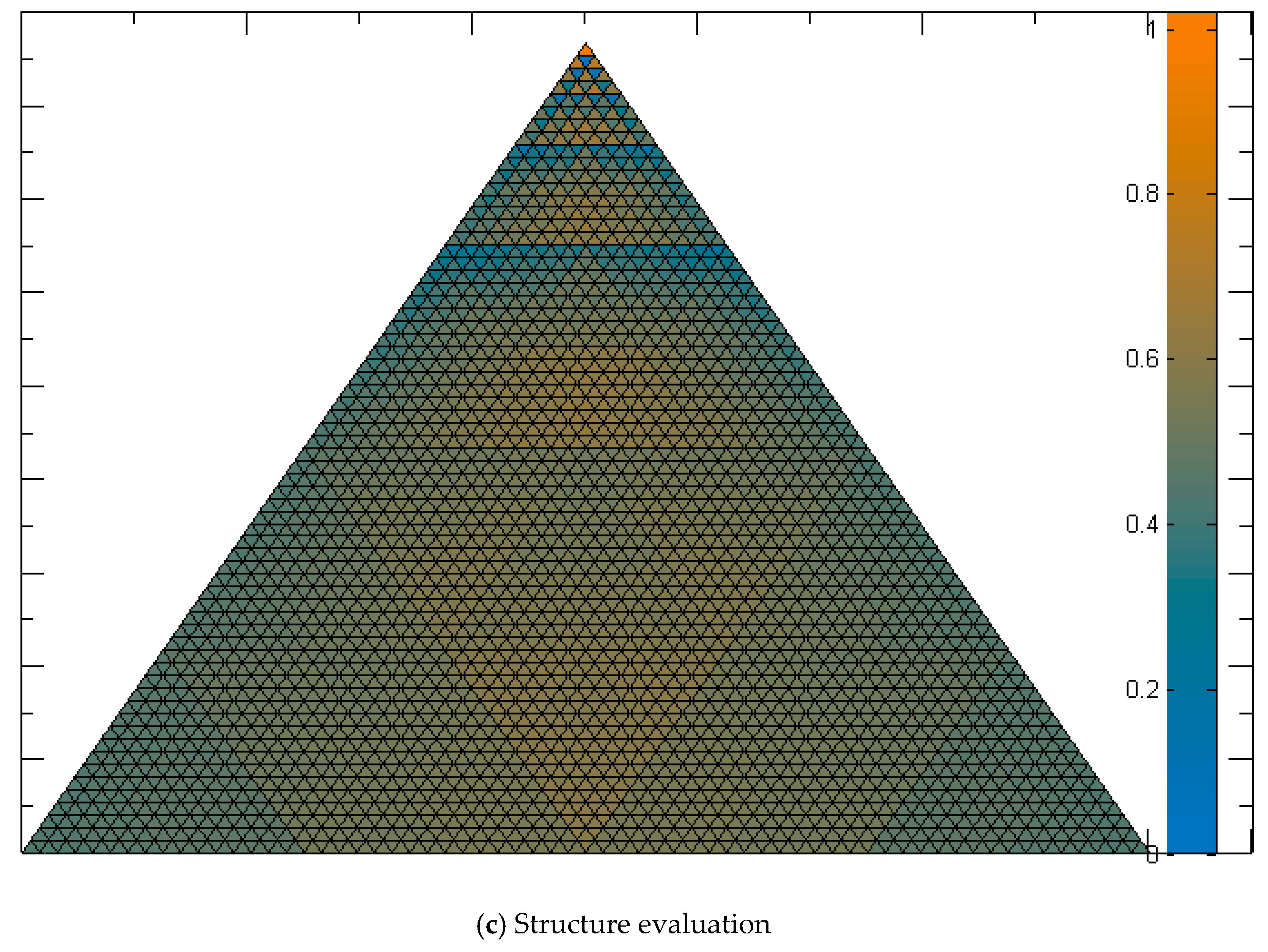
(2) The qualitative indicators were summarized by logical analysis, and four relatively independent evaluation indicators were extracted. Therefore, an independent quality evaluation indicator system of the DGG was reconstructed, including only six indicators or factors of Domain, Conversion, Hierarchy, Location, Area, Shape. The new indicator system covers all the information of the Goodchild Criteria in a clear, independent, and simple indicator system for the comprehensive quality evaluation of a DGG model. In the end, we took an octant of the QTM model as the test area and the visualization results conform to the correlation conclusions of the above quantitative indicator.
This article mainly used the QTM model as an example to reconstruct the quality evaluation indicator of the DGG. Although the triangle is the most basic shape, it has the main characteristics of other shapes. In future work, we will explore the specificity of the indicators of grid models in various shapes (such as triangular, quadrilateral, or hexagonal grid, etc.) and their influence on the quality evaluation system.


