
A Research on Susceptibility Mapping of Multiple Geological Hazards in Yanzi River Basin, China


Abstract
:1. Introduction
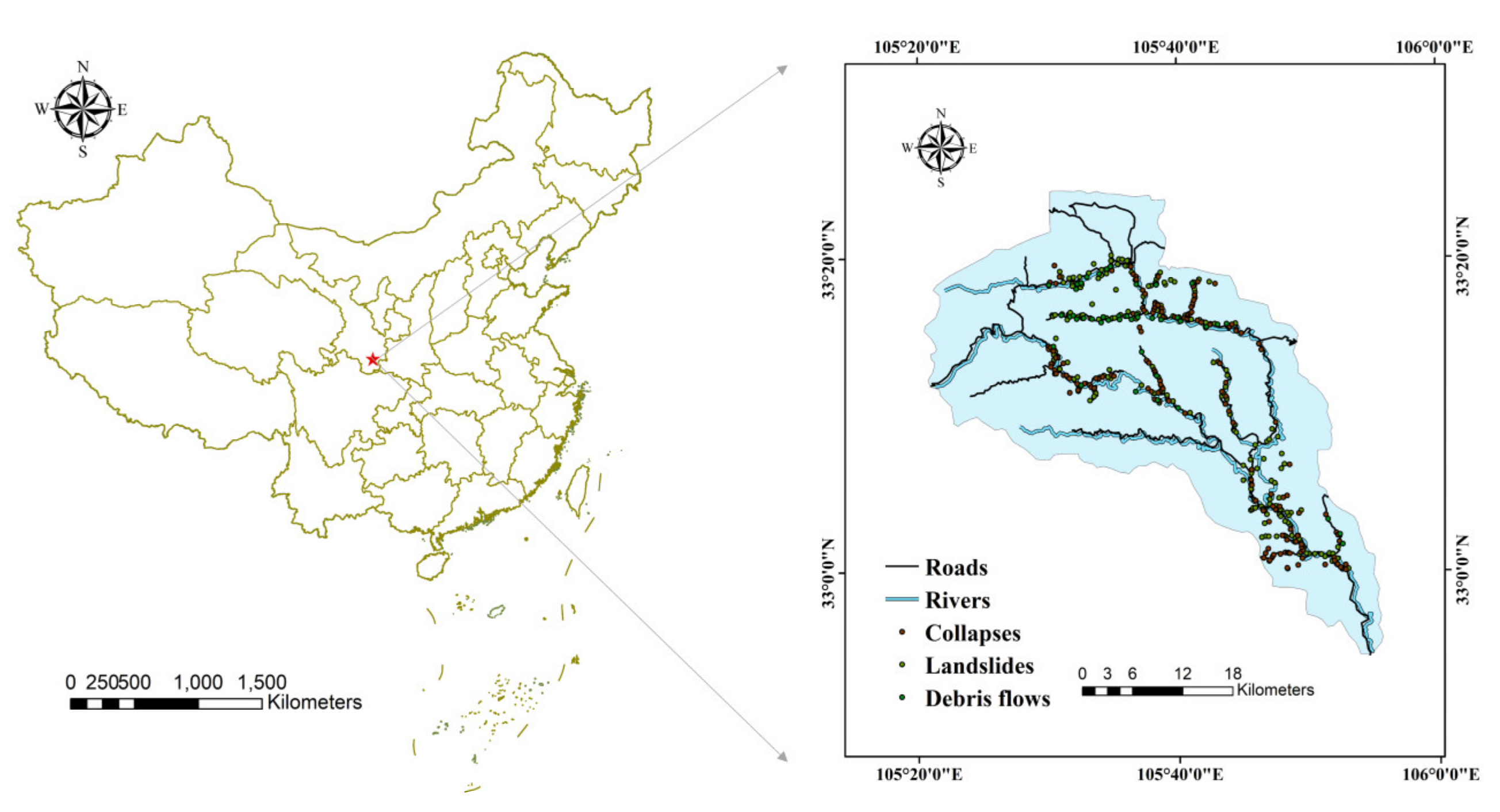
2. Study Area
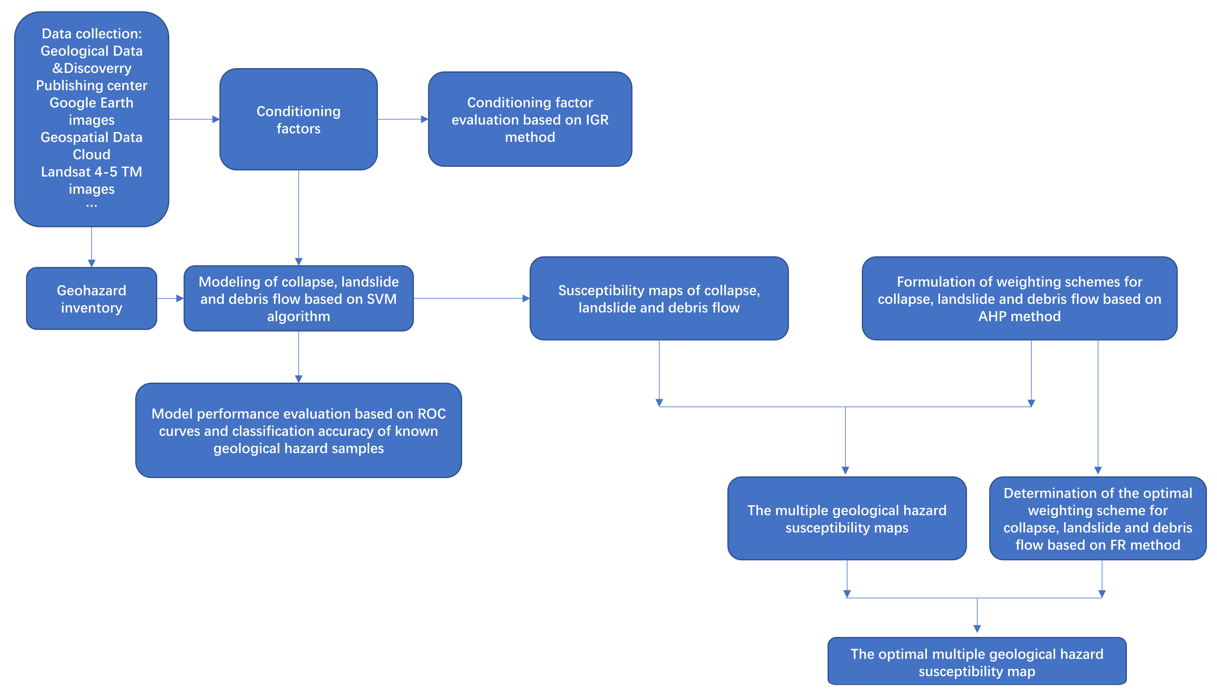
3. Materials and Methods
3.1. Geological Hazard Inventory
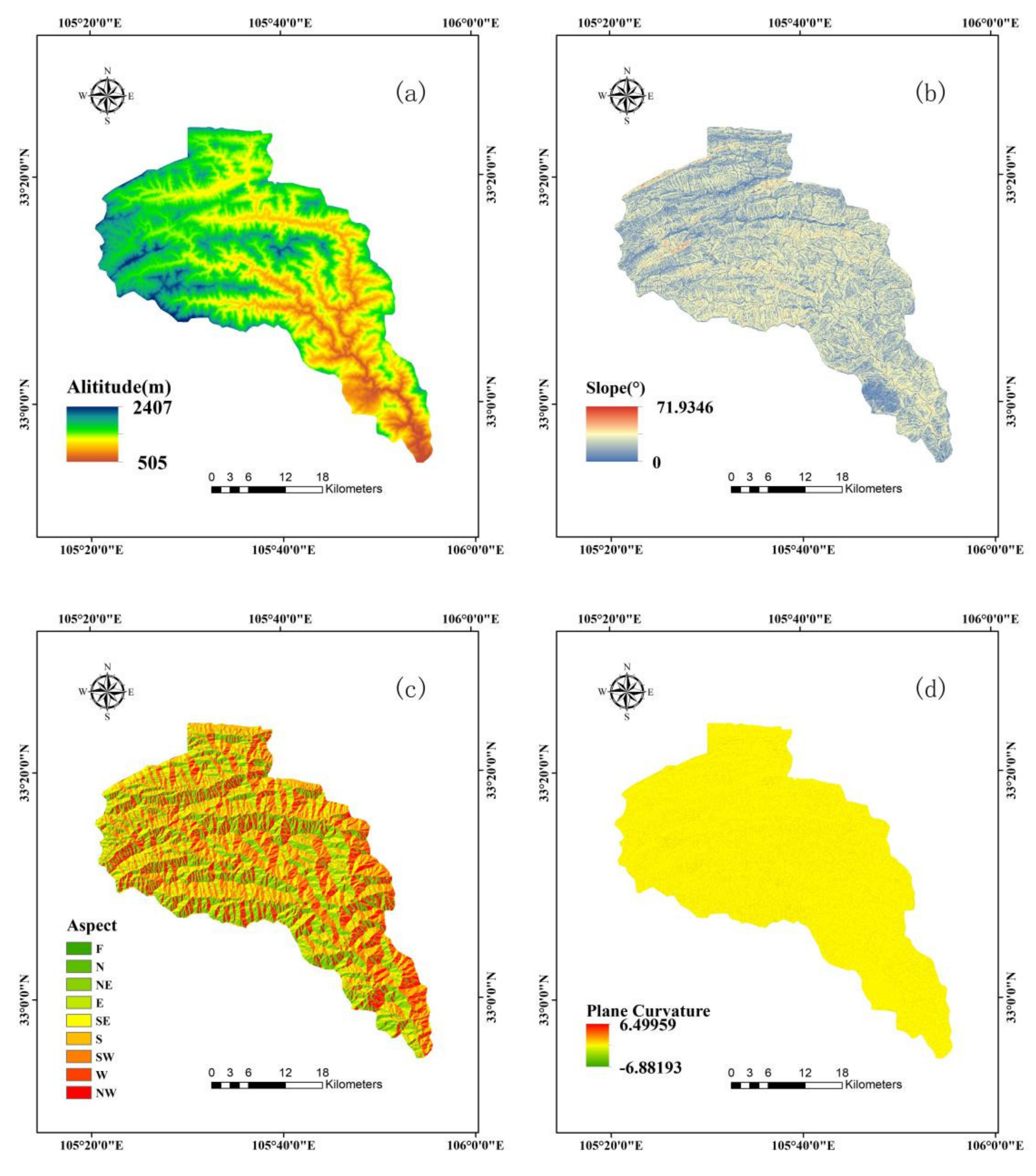
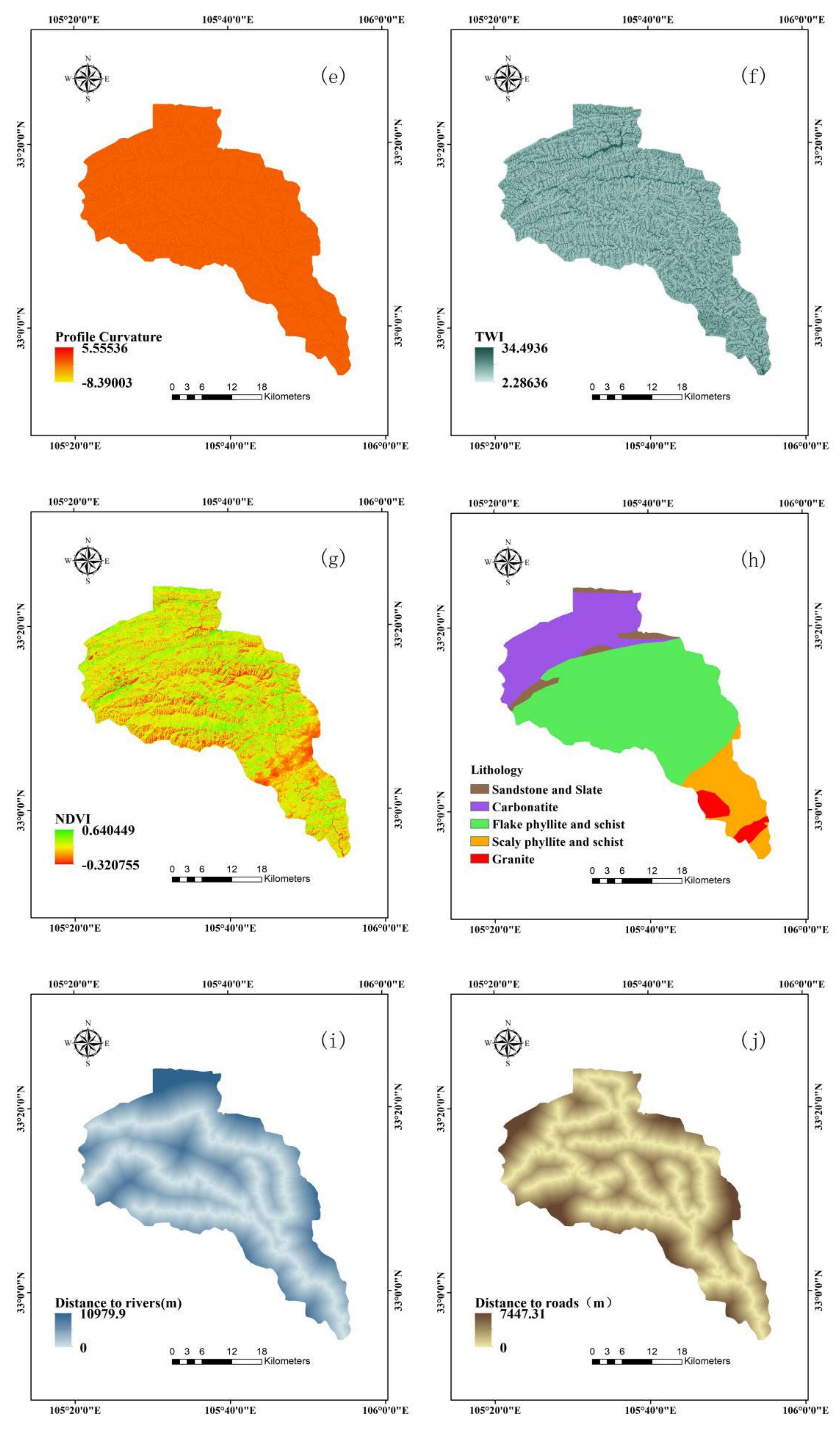
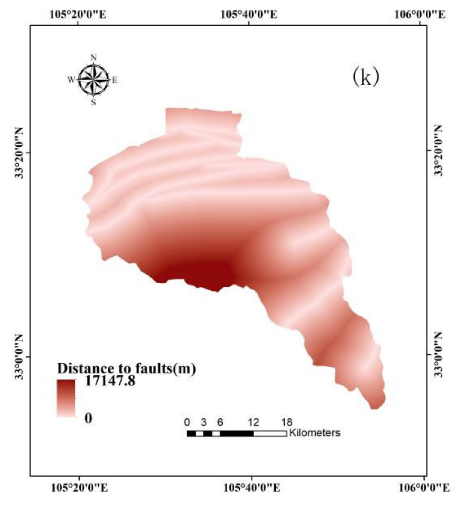
3.2. Conditioning Factors
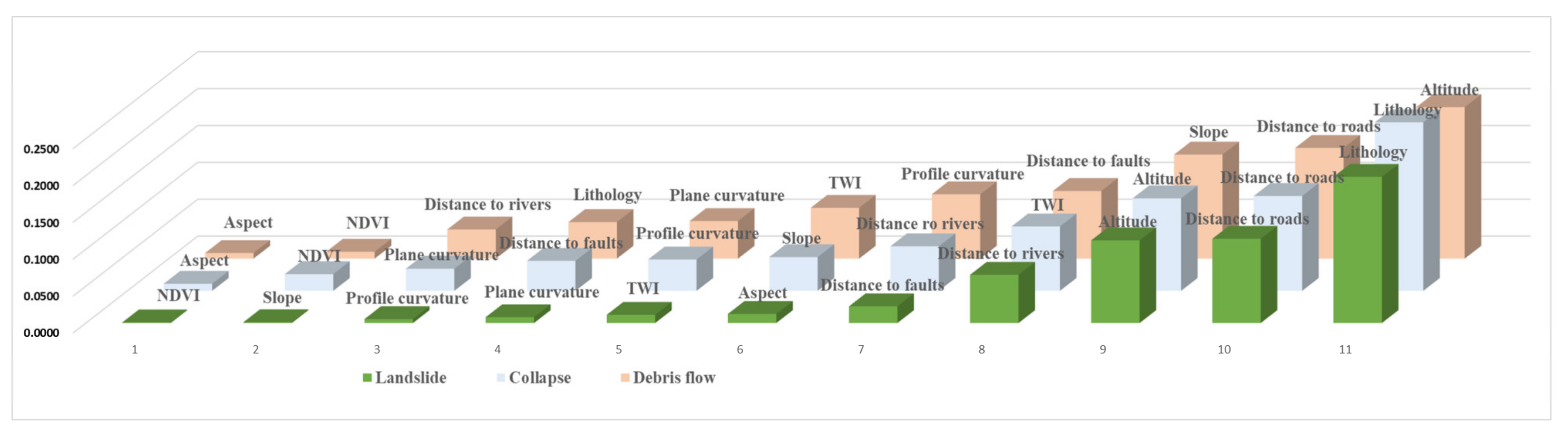
3.3. The Information Gain Ratio Method
3.4. Training and Validation Datasets
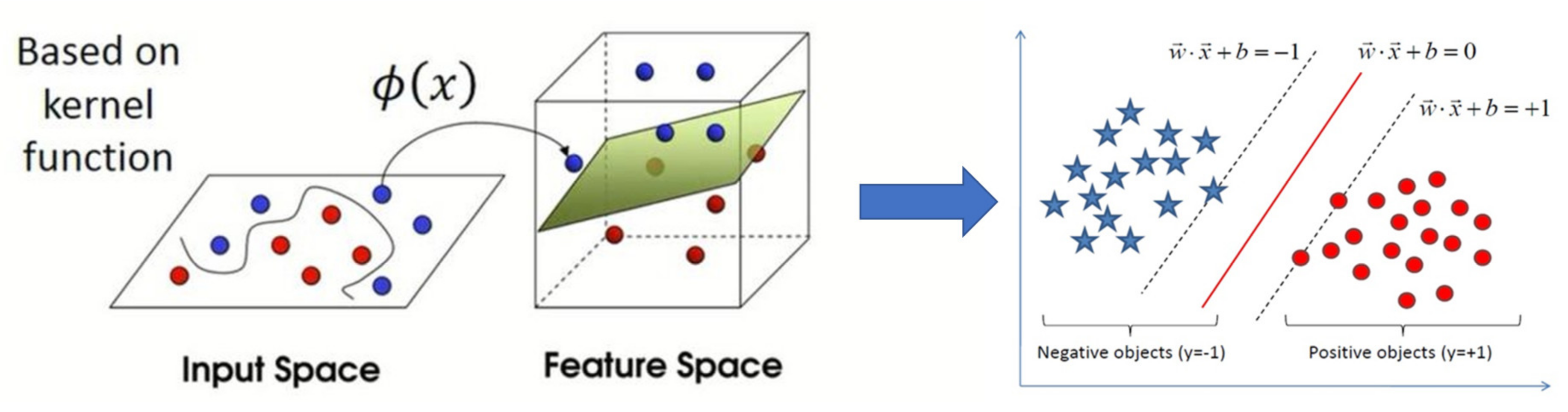
3.5. The Support Vector Machine Method
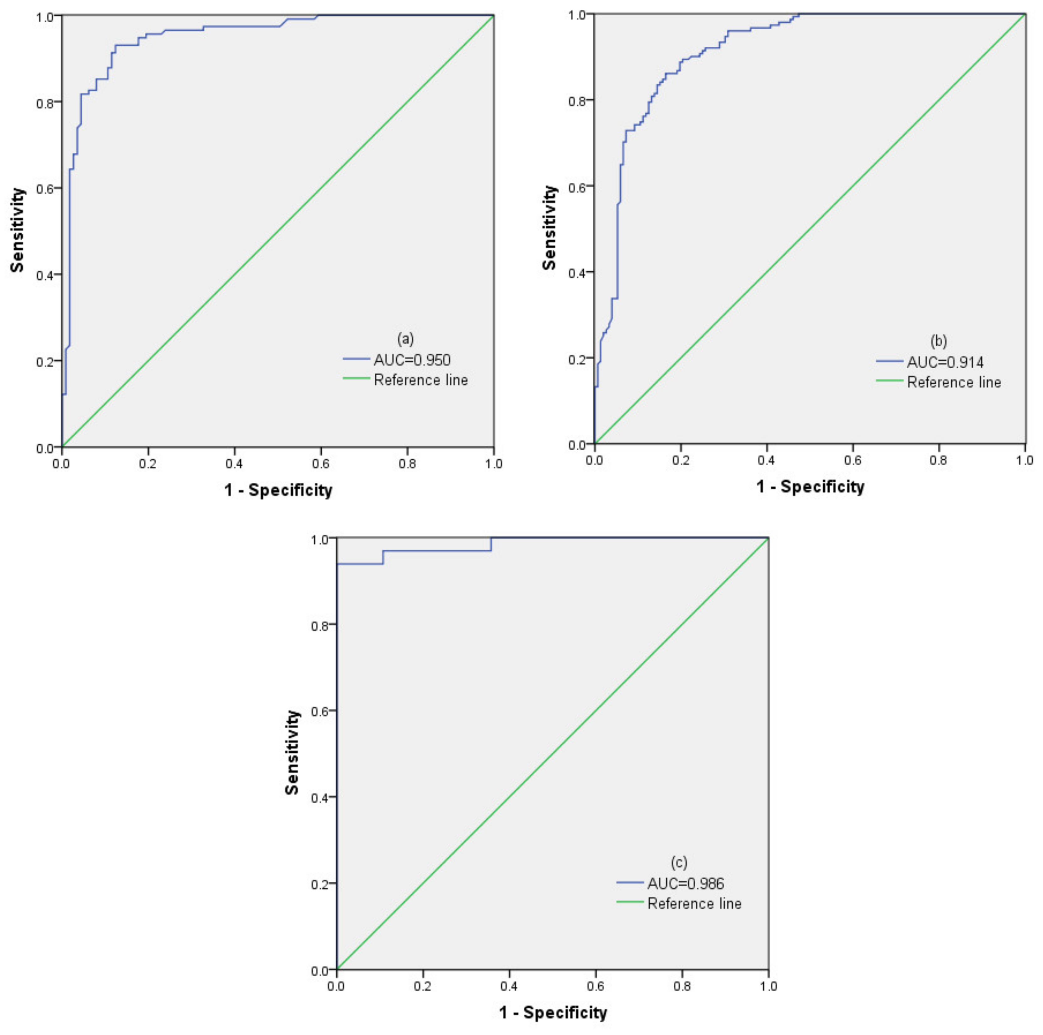
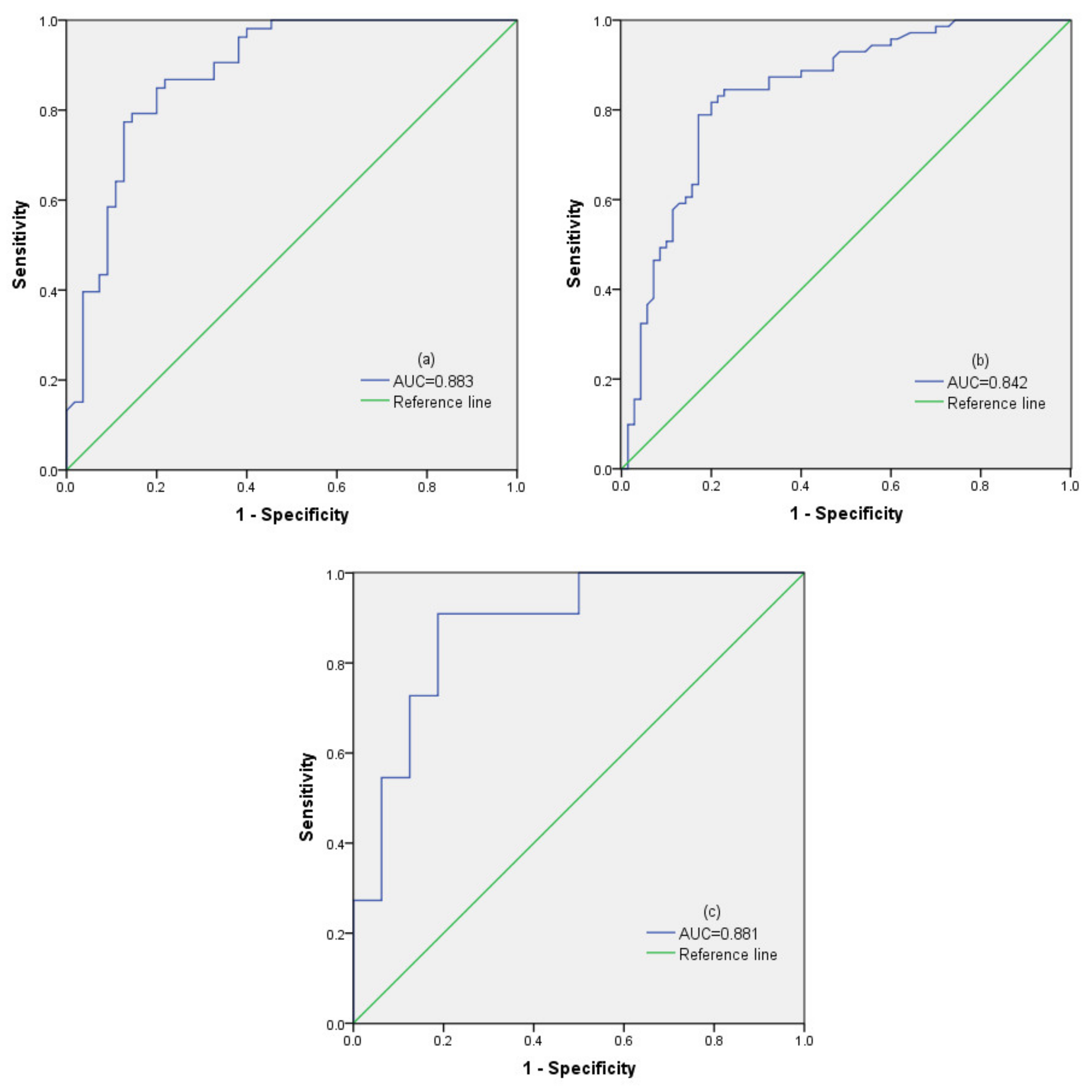
3.6. The ROC Curves
3.7. The AHP Method
- (a)
- Establishing a hierarchical structure model. In this paper, the purpose of applying the AHP method is to obtain the weights of collapse, landslide, and debris flow. The basic model of an analytic hierarchy was adopted, which can be divided into two layers: the target layer and the criterion layer.
- (b)
- Definition of comparative importance. It is the qualitative part of the AHP. In order to avoid complicated multi-factor comparisons, AHP compares the factors in pairs to improve the accuracy of the comparison. Satty [45] used a nine-point scale to perform the pair-wise comparison process. The definition of comparative importance was shown in Table 1. Since the research object of this paper is three different geological hazards, at the same time, in order to avoid the weight of a single geological hazard being too large or too small, we selected three adjacent relative importance scales of 1, 2, and 3.
- (c)
- Establishing the judgement matrix. The formula is as follows.where aij is the ratio of relative importance between two factors, and its value was obtained from Table 1.
- (d)
- Hierarchical ranking and its consistency check. The eigenvector corresponding to the largest eigenvalue λmax of the judgment matrix was normalized (The sum of the elements in the vector is 1) and then recorded as W. The element of W is the sorting weight of the relative importance of the element at the same level to the factor of the upper level. This process is called the hierarchical ranking. In order to check whether there are contradictions in the process of defining relative importance, the consistency check process is necessary, and the formula is as follows.where CI is the consistency index, λmax is the maximum eigenvalue of the judgement matrix A, and n is the order of the judgment matrix.where RI is the average random consistency, and it is associated with the order of the judgement matrix. The value can be obtained from Table 2. CR is the consistency ratio, and it is used in order to avoid the creation of any incidental judgment in the matrix. If CR < 0.1, the judgement matrix has a good consistency with reasonable judgement. Otherwise, the judgement matrix needs to be revised until the consistency test is satisfied [46].
3.8. The FR Method
3.9. The Superimposing Method for Susceptibility Maps
4. Results
4.1. The IGR Method Results
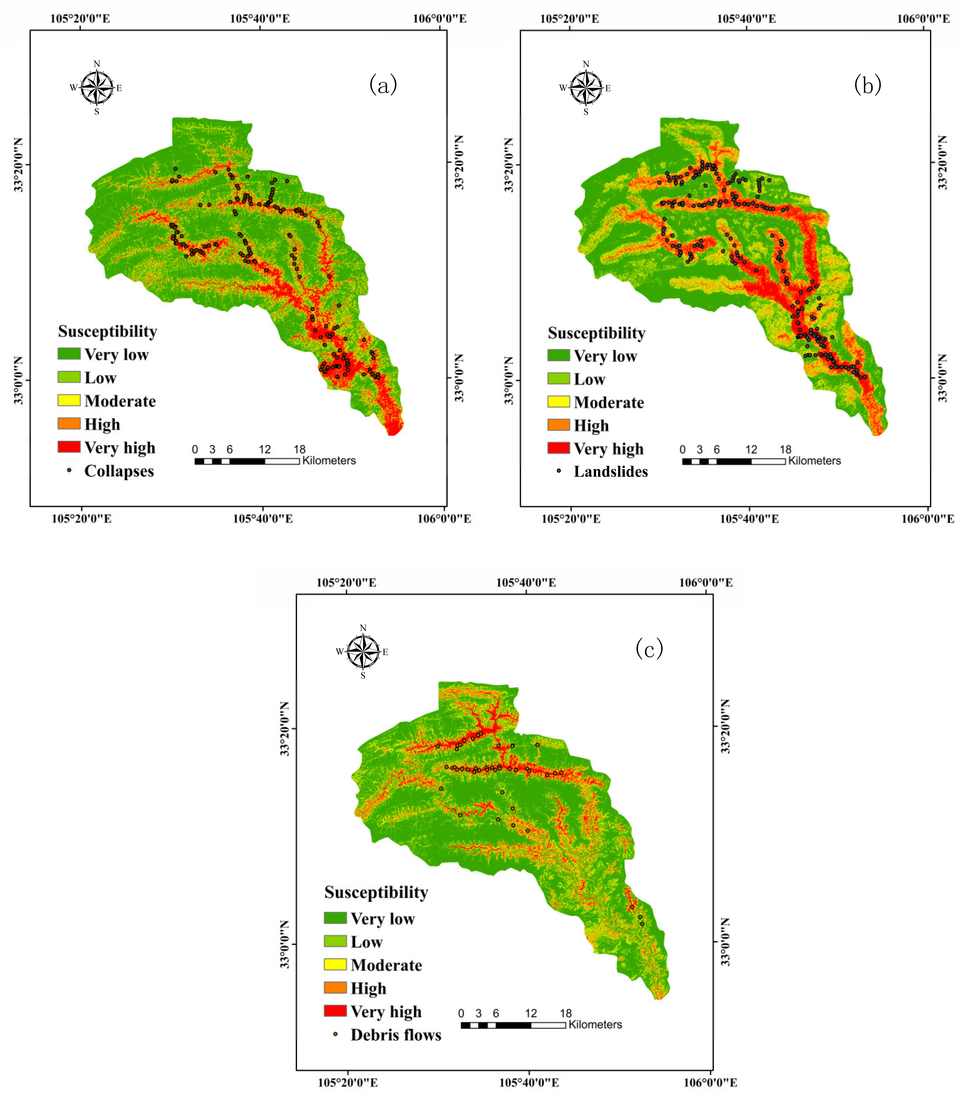
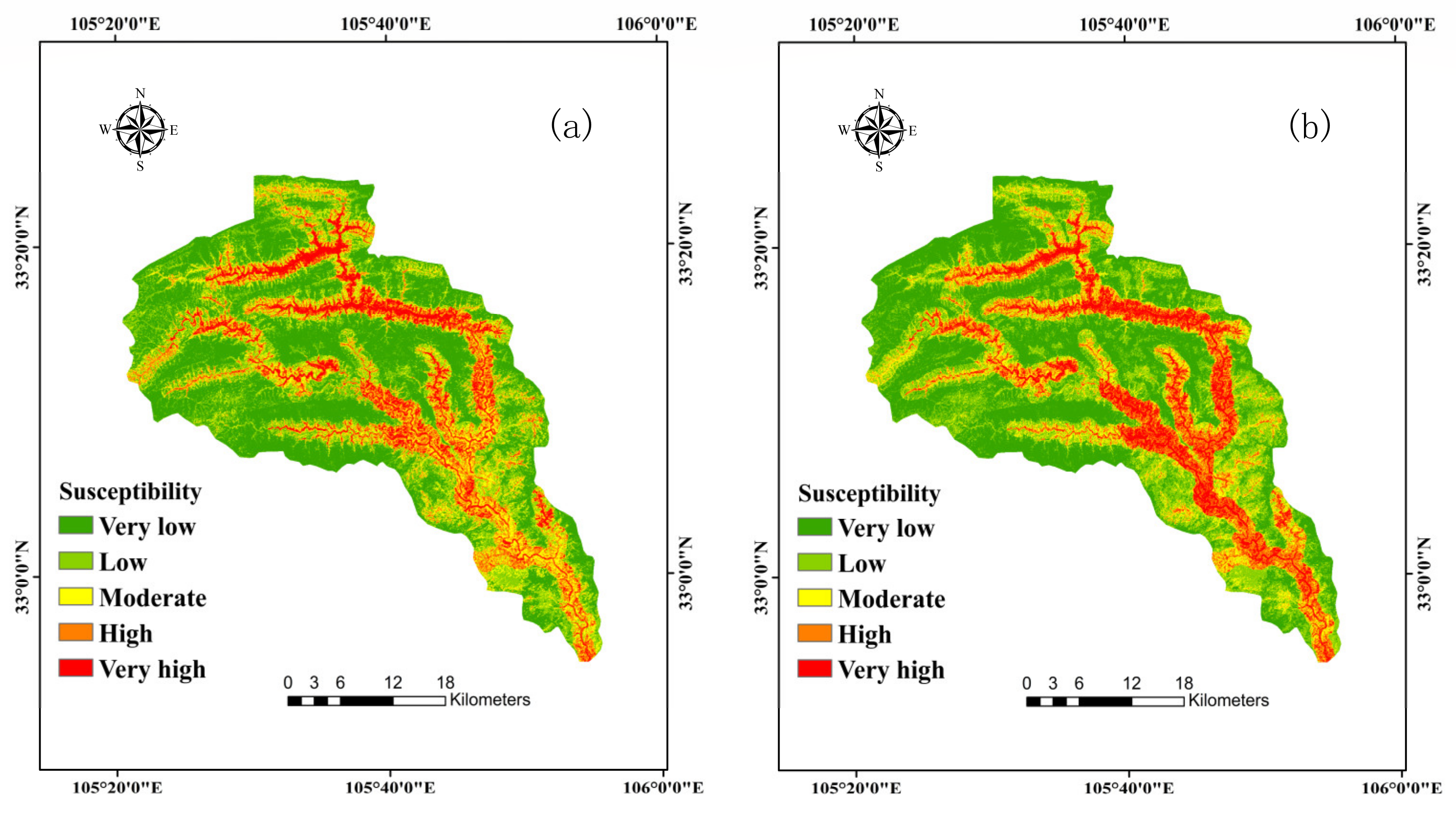
4.2. The Basic Geological Hazard Susceptibility Maps
4.3. Assessment of the Model Performance Using ROC Curves
4.4. The Weighting Schemes
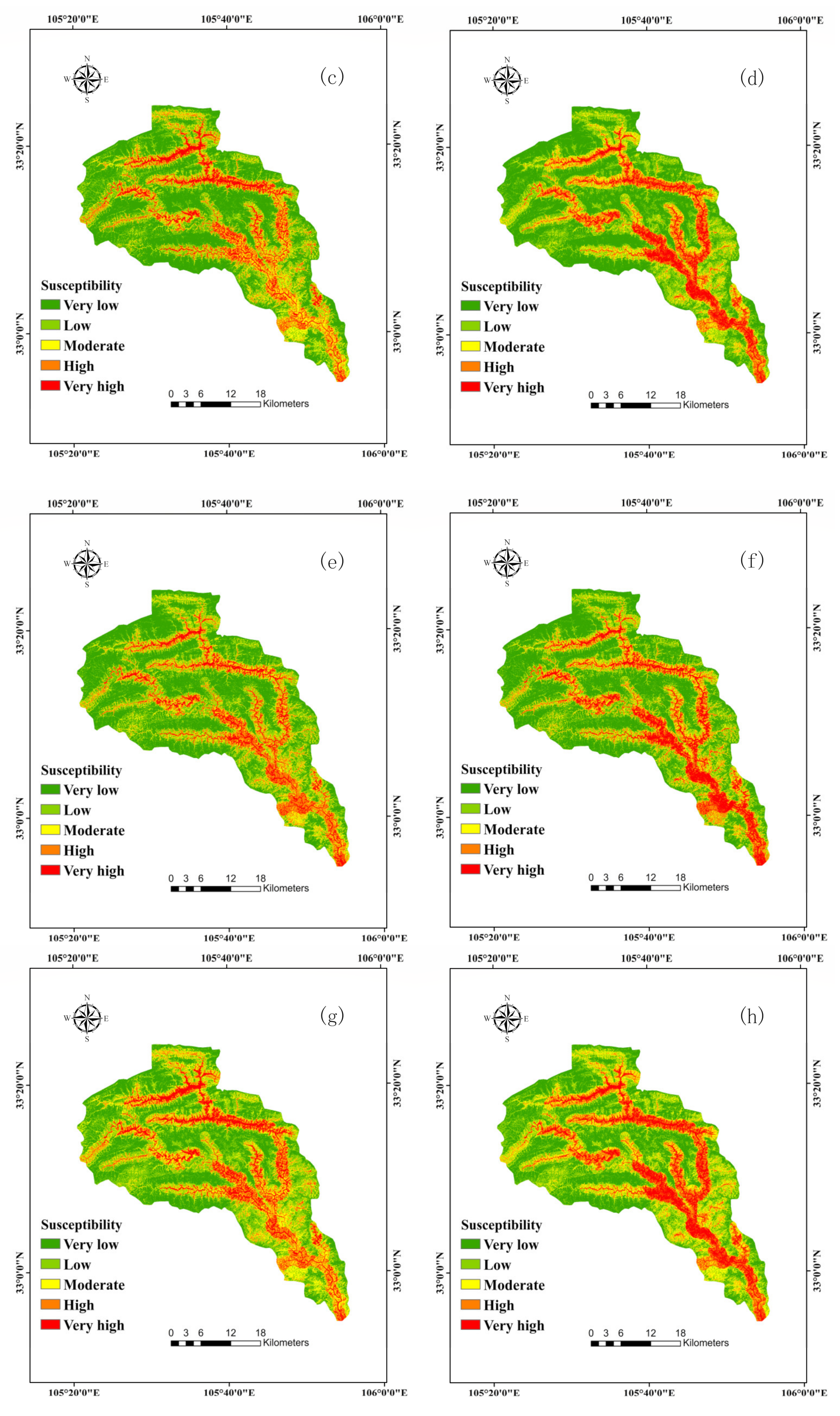
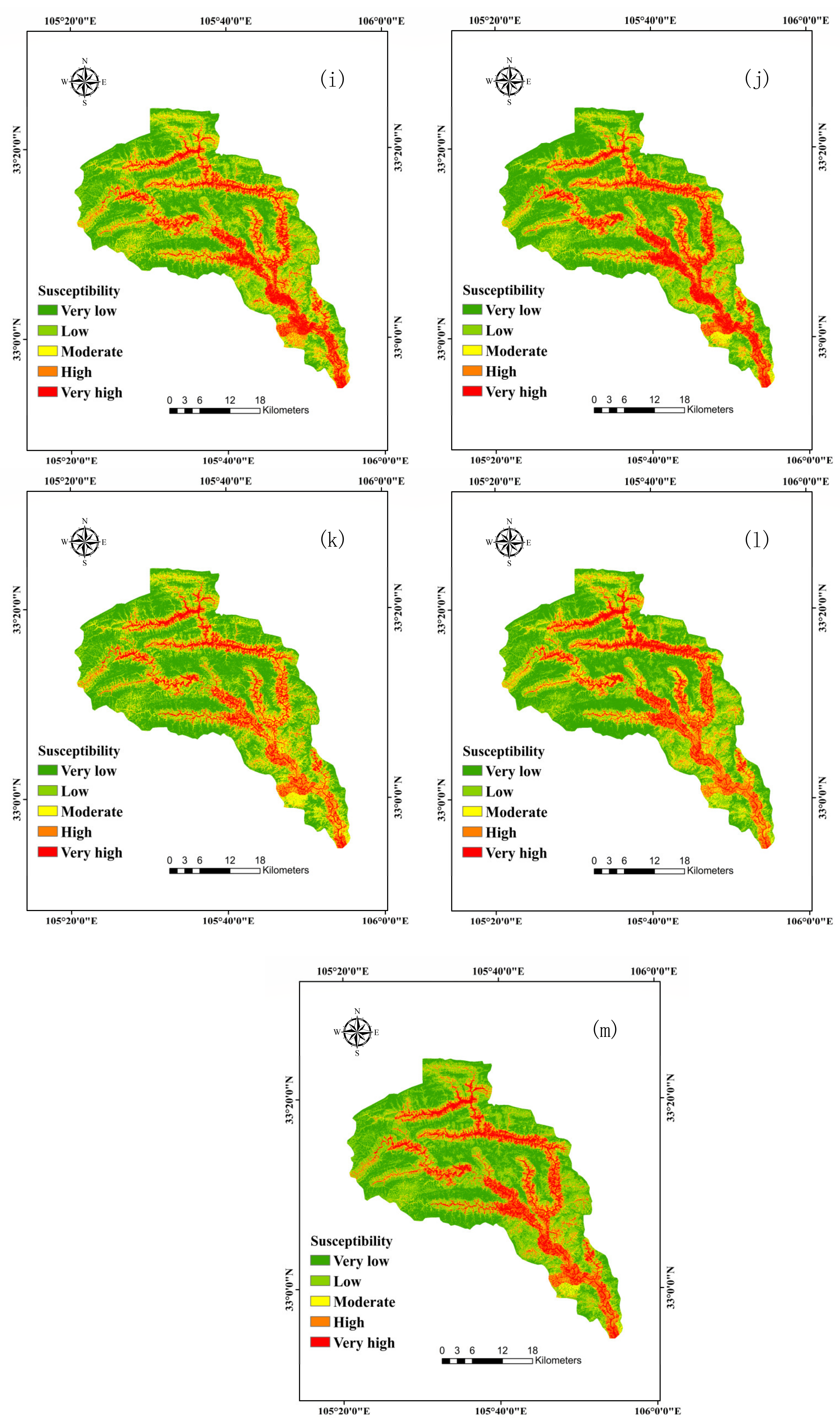
4.5. The Multiple Geological Hazard Susceptibility Maps
5. Discussion
5.1. Evaluation of Conditioning Factors
5.2. Evaluation of the Model Performance
5.3. Determination of the Optimal Weighting Scheme
5.4. Limitations
6. Conclusions
Author Contributions
Funding
Data Availability Statement
Acknowledgments
Conflicts of Interest
References
- Wang, J.J.; Yin, K.L.; Xiao, L.L. Landslide susceptibility assessment based on GIS and weighted information value: A case study of Wanzhou district, three gorges reservoir. Chin. J. Rock Mech. Eng. 2014, 33, 797–808. [Google Scholar] [CrossRef]
- Reichenbach, P.; Rossi, M.; Malamud, B.; Mihir, M.; Guzzetti, F. A review of statistically-based landslide susceptibility models. Earth Sci. Rev. 2018, 180, 60–91. [Google Scholar] [CrossRef]
- Corominas, J.; van Westen, C.; Frattini, P.; Casini, L.; Malet, J.-P.; Fotopoulou, S.; Catani, F.; Van Den Eeckhaut, M.; Mavrouli, O.; Agliardi, F.; et al. Recommendations for the quantitative analysis of landslide risk. Bull. Eng. Geol. Environ. 2014, 73, 209–263. [Google Scholar] [CrossRef]
- Yao, X.; Tham, L.G.; Dai, F.C. Landslide susceptibility mapping based on support vector machine: A case study on natural slopes of Hong Kong, China. Geomorphology. 2008, 101, 572–582. [Google Scholar] [CrossRef]
- Chang, K.T.; Merghadi, A.; Yunus, A.P.; Pham, B.T.; Dou, J. Evaluating scale effects of topographic variables in landslide susceptibility models using GIS-based machine learning techniques. Sci. Rep. 2019, 9, 12296. [Google Scholar] [CrossRef] [Green Version]
- Nguyen, M.D.; Pham, B.T.; Tuyen, T.; Yen, H.P.H.; Prakash, I.; Thanh, T.V.; Chapi, K.; Shirzadi, A.; Shahabi, H.; Dou, J.; et al. Development of an Artificial Intelligence Approach for Prediction of Consolidation Coefficient of Soft Soil: A Sensitivity Analysis. Open Constr. Build. Technol. 2019, 13. [Google Scholar] [CrossRef]
- Pham, B.T.; Prakash, I.; Dou, J.; Singh, S.K.; Trinh, P.T.; Tran, H.T.; Le, T.M.; Van, P.T.; Khoi, D.K.; Shirzadi, A.; et al. A novel hybrid approach of landslide susceptibility modelling using rotation forest ensemble and different base classifiers. Geocarto Int. 2019, 35, 1–25. [Google Scholar] [CrossRef]
- Tien, B.D.; Shirzadi, A.; Shahabi, H.; Geertsema, M.; Omidvar, E.; Clague, J.J.; Thai Pham, B.; Dou, J.; Talebpour, A.D.; Bin Ahmad, B.; et al. New Ensemble Models for Shallow Landslide Susceptibility Modeling in a Semi-Arid Watershed. Forests 2019, 10, 743. [Google Scholar] [CrossRef] [Green Version]
- Bergstra, J.; Yamins, D.; Cox, D.D. Making a Science of Model Search: Hyperparameter Optimization in Hundreds of Dimensions for Vision Architectures. In Proceedings of the 30th International Conference on Machine Learning, Atlanta, GE, USA, 16–21 June 2013. [Google Scholar]
- Khosravi, K.; Shahabi, H.; Pham, B.T.; Adamowski, J.; Shirzadi, A.; Pradhan, B.; Dou, J.; Ly, H.B.; Gróf, G.; Ho, H.L.; et al. A comparative assessment of flood susceptibility modeling using Multi-Criteria Decision-Making Analysis and Machine Learning Methods. J. Hydrol. 2019, 573, 311–323. [Google Scholar] [CrossRef]
- Pham, B.T.; Shirzadi, A.; Tien, B.D.; Prakash, I.; Dholakia, M.B. A hybrid machine learning ensemble approach based on a radial basis function neural network and rotation forest for landslide susceptibility modeling: A case study in the Himalayan area, India. Int. J. Sediment Res. 2018, 33, 157–170. [Google Scholar] [CrossRef]
- Chen, W.; Xie, X.; Peng, J.; Wang, J.; Duan, Z.; Hong, H. GIS-based landslide susceptibility modelling: A comparative assessment of kernel logistic regression, Naive-Bayes tree, and alternating decision tree models. Geomat. Nat. Haz. Risk 2017, 8, 950–973. [Google Scholar] [CrossRef] [Green Version]
- Wang, L.J.; Guo, M.; Sawada, K.; Lin, J.; Zhang, J. A comparative study of landslide susceptibility maps using logistic regression, frequency ratio, decision tree, weights of evidence and artificial neural network. Geosci. J. 2016, 20, 117–136. [Google Scholar] [CrossRef]
- Hong, H.; Pradhan, B.; Neamah Jebur, M.; Tien Bui, D.; Xu, C.; Akgun, A. Spatial prediction of landslide hazard at the Luxi area (China) using support vector machines. Environ. Earth Sci. 2016, 75, 40. [Google Scholar] [CrossRef]
- Liang, Z.; Wang, C.M.; Han, S.L.; Kaleem, U.J.K.; Liu, Y.A. Classification and susceptibility assessment of debris flow based on a semi-quantitative method combination of the fuzzy C-means algorithm, factor analysis and efficacy coefficient. Nat. Hazards Earth Syst. Sci. 2020, 20, 1287–1304. [Google Scholar] [CrossRef]
- Oh, H.J.; Lee, S. Shallow Landslide Susceptibility Modeling Using the Data Mining Models Artificial Neural Network and Boosted Tree. Appl. Sci. 2017, 7. [Google Scholar] [CrossRef] [Green Version]
- Pham, B.T.; Nguyen-Thoi, T.; Qi, C.C.; Phong, T.V.; Dou, J.; Lanh, S.H.; Hiep, V.L.; Prakash, I. Coupling RBF neural network with ensemble learning techniques for landslide susceptibility mapping. Catena 2020, 195, 104805. [Google Scholar] [CrossRef]
- Merghadi, A.; Yunus, A.P.; Dou, J.; Whiteley, J.; Thai, P.B.; Bui, D.T.; Avtar, R.; Abderrahmane, B. Machine learning methods for landslide susceptibility studies: A comparative overview of algorithm performance. Earth Sci. Rev. 2020, 207, 103225. [Google Scholar] [CrossRef]
- Gruber, F.E.; Mergili, M. Regional-scale analysis of high-mountain multi-hazard and risk indicators in the Pamir (Tajikistan) with GRASS GIS. Nat. Hazards Earth Syst. Sci. 2013, 13, 2779–2796. [Google Scholar] [CrossRef] [Green Version]
- Marzocchi, W.; Garcia-Aristizabal, A.; Gasparini, P.; Mastellone, M.L.; Di, R.A. Basic principles of multi-risk assessment: A case study in Italy. Nat. Hazards. 2012, 62, 551–573. [Google Scholar] [CrossRef]
- Tate, E.; Cutter, S.L.; Berry, M. Integrated multihazard mapping. Environ. Plann. B Plann. Des. 2010, 37, 646–663. [Google Scholar] [CrossRef] [Green Version]
- Gallina, V.; Torresan, S.; Critto, A.; Sperotto, A.; Glade, T.; Marcomini, A. A review of multirisk methodologies for natural hazards: Consequences and challenges for a climate change impact assessment. J. Environ. Manag. 2016, 168, 123–132. [Google Scholar] [CrossRef]
- Carpignano, A.; Golia, E.; Di, M.C.; Bouchon, S.; Nordvik, J.P. A methodological approach for the definition of multi-risk maps at regional level: First application. J. Risk Res. 2009, 12, 513–534. [Google Scholar] [CrossRef]
- Zhang, L.; Zhang, S. Approaches to multi-hazard landslide risk assessment. In Proceedings of the Geo-risk Conference, Denver, CO, USA, 4–7 June 2017. [Google Scholar]
- Sun, L.; Ma, C.; Li, Y. Multiple geo-environmental hazards susceptibility assessment: A case study in Luoning County, Henan Province, China. Geomat. Nat. Hazards Risk. 2019, 10, 2009–2029. [Google Scholar] [CrossRef]
- Bathrellos, G.D.; Skilodimou, H.D.; Chousianitis, K.; Youssef, A.M.; Pradhan, B. Suitability estimation for urban development using multi-hazard assessment map. Sci. Total Environ. 2017, 575, 119–134. [Google Scholar] [CrossRef]
- Ye, Z.N.; Yang, Q.; Li, Q.; Zhang, X.H. Landslide characteristics and hazard assessment in Yanzi River Basin. J. Liaoning Tech. Univ. (Nat. Sci.) 2020, 39, 145–151. [Google Scholar] [CrossRef]
- Yang, Q.; YE, Z.N.; Gao, Y.L.; Li, Q.; Ding, W.C. Dataset of the 2015 Geo-Hazard Survey of the Yanzi River Basin, Upstream of the Jialing River. Geol. China. 2018, 45, 156–167. [Google Scholar]
- Yang, Q.; Wang, S.Y.; Ye, Z.N. Analysis on the development of geological hazard and failure mode in Yanzi River Basin. J. Eng. Geol. 2019, 27, 289–295. [Google Scholar] [CrossRef]
- Pradhan, A.M.S.; Kim, Y.T. Relative effect method of landslide susceptibility zonation in weathered granite soil: A case study in Deokjeok-ri Creek, South Korea. Nat. Hazards 2014, 72, 1189–1217. [Google Scholar] [CrossRef]
- Varnes, D.J. Landslide Hazard Zonation: A Review of Principles and Practice; United Nations: Paris, France, 1984; p. 63. [Google Scholar]
- Pourghasemi, H.R.; Mohammady, M.; Pradhan, B. Landslide susceptibility mapping using index of entropy and conditional probability models in GIS: Safarood Basin, Iran. Catena 2012, 97, 71–84. [Google Scholar] [CrossRef]
- Oh, H.J.; Pradhan, B. Application of a neuro-fuzzy model to landslide-susceptibility mapping for shallow landslides in a tropical hilly area. Comput. Geosci. 2011, 37, 1264–1276. [Google Scholar] [CrossRef]
- Pourghasemi, H.R.; Jirandeh, A.G.; Pradhan, B.; Xu, C.; Gokceoglu, C. Landslide susceptibility mapping using support vector machine and GIS at the Golestan Province, Iran. J. Earth Syst. Sci. 2013, 122, 349–369. [Google Scholar] [CrossRef] [Green Version]
- Bui, D.T.; Ho, T.C.; Pradhan, B.; Pham, B.T.; Nhu, V.H.; Revhaug, I. GIS-based modeling of rainfall-induced landslides using data mining-based functional trees classifier with AdaBoost, Bagging, and MultiBoost ensemble frameworks. Environ. Earth Sci. 2016, 75, 22. [Google Scholar] [CrossRef]
- Dou, J.; Yunus, A.P.; Bui, D.T.; Merghadi, A.; Sahana, M.; Zhu, Z.F.; Chen, C.W.; Han, Z.; Pham, B.T. Improved landslide assessment using support vector machine with bagging, boosting, and stacking ensemble machine learning framework in a mountainous watershed, Japan. Landslides 2020, 17, 641–658. [Google Scholar] [CrossRef]
- Guzzetti, F.; Reichenbach, P.; Ardizzone, F.; Cardinali, M.; Galli, M. Estimating the quality of landslide susceptibility models. Geomorphology 2006, 81, 166–184. [Google Scholar] [CrossRef]
- Guzzetti, F.; Galli, M.; Reichenbach, P.; Ardizzone, F.; Cardinali, M. Landslide hazard assessment in the Collazzone area, Umbria, central Italy. Nat. Hazard. Earth Syst. Sci. 2006, 6, 115–131. [Google Scholar] [CrossRef]
- Xu, C.; Dai, F.; Xu, X.; Lee, Y.H. GIS-based support vector machine modeling of earthquake-triggered landslide susceptibility in the Jianjiang River watershed, China. Geomorphology 2012, 145, 70–80. [Google Scholar] [CrossRef]
- Provost, F.; Fawcett, T. Robust classification for imprecise environments. Mach. Learn. 2001, 42, 203–231. [Google Scholar] [CrossRef]
- Chen, W.; Pourghasemi, H.R.; Naghibi, S.A. A comparative study of landslide susceptibility maps produced using support vector machine with different kernel functions and entropy data mining models in China. Bull. Eng. Geol. Environ. 2018, 77, 647–664. [Google Scholar] [CrossRef]
- Karaman, H.; Erden, T. Net earthquake hazard and elements at risk (NEaR) map creation for city of Istanbul via spatial multi-criteria decision analysis. Nat. Hazards 2014, 73, 685–709. [Google Scholar] [CrossRef]
- Rozos, D.; Bathrellos, G.D.; Skilodimou, H.D. Comparison of the implementation of rock engineering system (RES) and analytic hierarchy process (AHP) methods, based on landslide susceptibility maps, compiled in GIS environment. A case study from the eastern Achaia County of Peloponnesus, Greece. Environ. Earth Sci. 2011, 63, 49–63. [Google Scholar] [CrossRef]
- Peng, S.H.; Shieh, M.J.; Fan, S.Y. Potential hazard map for disaster prevention using GIS-based linear combination approach and analytic hierarchy method. J. Geogr. Inf. Syst. 2012, 4, 403–411. [Google Scholar] [CrossRef] [Green Version]
- Saaty, T.L. A scaling method for priorities in hierarchical structures. Math. Psychol. 1977, 15, 234–281. [Google Scholar] [CrossRef]
- Saaty, T.L. How to make a decision: The analytic hierarchy process. Eur. J. Oper. Res. 1990, 48, 9–26. [Google Scholar] [CrossRef]
- Delmonaco, G.; Margottini, C.; Spizzichino, D. New Methodology for Multi-Risk Assessment and the Harmonisation of Different Natural Risk Maps; Armonia Project: Rome, Italy, 2006. [Google Scholar]
- Dai, F.; Lee, C.; Ngai, Y. Landslide risk assessment and management: An overview. Eng. Geol. 2002, 64, 65–87. [Google Scholar] [CrossRef]
- Bathrellos, G.D.; Gaki-Papanastassiou, K.; Skilodimou, H.D.; Skianis, G.A.; Chousianitis, K.G. Assessment of rural community and agricultural development using geomorphological–geological factors and GIS in the Trikala prefecture (Central Greece). Stoch. Environ. Res. Risk A 2013, 27, 573–588. [Google Scholar] [CrossRef]


| 1 | Two factors are equally important |
| 3 | One factor is more important |
| 5 | One factor is strongly more important |
| 7 | One factor is very strongly more important |
| 9 | One factor is extremely more important |
| 2, 4, 6,8 | Intermediate values |
| n | 1 | 2 | 3 | 4 | 5 | 6 | 7 | 8 | 9 | 10 | 11 | 12 |
|---|---|---|---|---|---|---|---|---|---|---|---|---|
| RI | 0 | 0 | 0.52 | 0.89 | 1.12 | 1.26 | 1.36 | 1.41 | 1.46 | 1.49 | 1.52 | 1.54 |
| Probability Level | Score |
|---|---|
| Very low | 1 |
| Low | 2 |
| Moderate | 3 |
| High | 4 |
| Very high | 5 |
| Groups | No. of Collapses | Percentage of Collapses | No. of Landslides | Percentage of Landslides | No. of Debris Flows | Percentage of Debris Flows |
|---|---|---|---|---|---|---|
| Very low | 8 | 4.7% | 11 | 5.0% | 0 | 0.0% |
| Low | 6 | 3.5% | 7 | 3.2% | 2 | 4.5% |
| Moderate | 15 | 8.8% | 30 | 13.5% | 3 | 6.8% |
| High | 28 | 16.5% | 40 | 18.0% | 4 | 9.1% |
| Very high | 113 | 66.5% | 134 | 60.3% | 35 | 79.5% |
| A 1 | A 2 | ||||||
| Element | Hazard 1 | Hazard 2 | Hazard 3 | Element | Hazard 1 | Hazard 2 | Hazard3 |
| Hazard 1 | 1 | 0.5 | 0.33 | Hazard 1 | 1 | 1 | 0.5 |
| Hazard 2 | 2 | 1 | 0.5 | Hazard 2 | 1 | 1 | 0.5 |
| Hazard 3 | 3 | 2 | 1 | Hazard 3 | 2 | 2 | 1 |
| A 3 | A 4 | ||||||
| Element | Hazard 1 | Hazard 2 | Hazard 3 | Element | Hazard 1 | Hazard 2 | Hazard3 |
| Hazard 1 | 1 | 0.5 | 0.5 | Hazard 1 | 1 | 1 | 1 |
| Hazard 2 | 2 | 1 | 1 | Hazard 2 | 1 | 1 | 1 |
| Hazard 3 | 2 | 1 | 1 | Hazard 3 | 1 | 1 | 1 |
| Types of Weighting Schemes | Weighting Schemes | Weight of Collapse | Weight of Landslide | Weight of Debris Flow | CI | RI | CR |
|---|---|---|---|---|---|---|---|
| 1 | a | 0.164 | 0.297 | 0.539 | 0.005 | 0.52 | 0.009 |
| b | 0.164 | 0.539 | 0.297 | ||||
| c | 0.297 | 0.164 | 0.539 | ||||
| d | 0.297 | 0.539 | 0.164 | ||||
| e | 0.539 | 0.164 | 0.297 | ||||
| f | 0.539 | 0.297 | 0.164 | ||||
| 2 | g | 0.250 | 0.250 | 0.500 | 0 | 0 | |
| h | 0.250 | 0.500 | 0.250 | ||||
| i | 0.500 | 0.250 | 0.250 | ||||
| 3 | j | 0.400 | 0.400 | 0.200 | 0 | 0 | |
| k | 0.400 | 0.200 | 0.400 | ||||
| l | 0.200 | 0.400 | 0.400 | ||||
| 4 | m | 0.333 | 0.333 | 0.333 | 0 | 0 |
| Maps | Map 1 | Map 2 | Map 3 | Map 4 | Map 5 | Map 6 | Map 7 | Map 8 | Map 9 | Map 10 | Map 11 | Map 12 | Map 13 | |
|---|---|---|---|---|---|---|---|---|---|---|---|---|---|---|
| Susceptibility | ||||||||||||||
| Very low | 42.0% | 40.0% | 42.0% | 40.0% | 41.5% | 41.5% | 31.4% | 31.4% | 31.4% | 35.4% | 37.5% | 35.9% | 31.4% | |
| Low | 20.6% | 23.2% | 21.0% | 23.1% | 23.3% | 20.6% | 25.8% | 24.6% | 25.6% | 25.1% | 24.2% | 25.0% | 34.7% | |
| Moderate | 16.2% | 13.7% | 16.1% | 13.6% | 14.8% | 14.2% | 19.2% | 17.5% | 17.7% | 13.8% | 17.5% | 14.0% | 8.2% | |
| High | 12.3% | 12.5% | 12.2% | 12.3% | 12.2% | 11.7% | 13.3% | 13.8% | 12.8% | 13.4% | 11.0% | 15.1% | 14.2% | |
| Very high | 8.8% | 10.7% | 8.7% | 11.1% | 8.2% | 12.0% | 10.3% | 12.7% | 12.5% | 12.3% | 9.8% | 10.0% | 11.5% | |
| Factors | Class | No. of Landslide | Percentage of Landslide | No. of Collapse | Percentage of Collapse | No. of Debris Flow | Percentage of Debris Flow |
|---|---|---|---|---|---|---|---|
| Altitude (m) | <1000 | 79 | 35.5 | 61 | 36.3 | 4 | 9.1 |
| 1000–1300 | 87 | 39.2 | 73 | 43.5 | 35 | 79.5 | |
| 1300–1600 | 55 | 24.8 | 34 | 20.2 | 5 | 11.4 | |
| 1600–1900 | 1 | 0.5 | 0 | 0 | 0 | 0.0 | |
| >1900 | 0 | 0 | 0 | 0 | 0 | 0.0 | |
| Slope (°) | <15 | 33 | 14.9 | 72 | 42.8 | 25 | 56.8 |
| 15–24 | 79 | 35.6 | 39 | 23.2 | 18 | 40.9 | |
| 24–33 | 80 | 36 | 30 | 17.9 | 1 | 2.3 | |
| >33 | 30 | 13.5 | 27 | 16.1 | 0 | 0.0 | |
| Aspect | Flat | 0 | 0 | 0 | 0 | 0 | 0.0 |
| North | 19 | 8.5 | 11 | 6.5 | 10 | 22.7 | |
| North east | 39 | 17.6 | 40 | 23.9 | 8 | 18.2 | |
| East | 20 | 9 | 22 | 13.1 | 2 | 4.5 | |
| South east | 39 | 17.6 | 23 | 13.7 | 5 | 11.4 | |
| South | 49 | 22.1 | 14 | 8.3 | 5 | 11.4 | |
| Southwest | 31 | 14 | 25 | 14.9 | 7 | 15.9 | |
| West | 15 | 6.8 | 18 | 10.7 | 4 | 9.1 | |
| Northwest | 10 | 4.4 | 15 | 8.9 | 3 | 6.8 | |
| Plan curvature | <−0.4 | 7 | 3.2 | 13 | 7.7 | 5 | 11.4 |
| −0.4–0 | 90 | 40.5 | 101 | 60.1 | 26 | 59.1 | |
| 0–0.4 | 101 | 45.5 | 46 | 27.4 | 13 | 29.5 | |
| >0.4 | 24 | 10.8 | 8 | 4.8 | 0 | 0.0 | |
| Profile curvature | <−0.5 | 8 | 3.6 | 5 | 3 | 0 | 0.0 |
| −0.5–0 | 73 | 32.9 | 42 | 25 | 6 | 13.6 | |
| 0–0.5 | 119 | 53.6 | 89 | 53 | 31 | 70.5 | |
| >0.5 | 22 | 9.9 | 32 | 19 | 7 | 15.9 | |
| TWI | <5 | 77 | 34.7 | 27 | 16.1 | 3 | 6.8 |
| 5–7 | 90 | 40.5 | 68 | 40.5 | 18 | 40.9 | |
| 7–11 | 49 | 22.1 | 56 | 33.3 | 15 | 34.1 | |
| >11 | 6 | 2.7 | 17 | 10.1 | 8 | 18.2 | |
| Lithology | 1 | 3 | 1.3 | 3 | 1.7 | 0 | 0.0 |
| 2 | 42 | 18.9 | 10 | 6 | 12 | 27.3 | |
| 3 | 115 | 51.8 | 108 | 64.3 | 0 | 0.0 | |
| 4 | 59 | 26.7 | 31 | 18.5 | 29 | 65.9 | |
| 5 | 3 | 1.3 | 16 | 9.5 | 3 | 6.8 | |
| NDVI | <0.1 | 35 | 15.8 | 43 | 25.6 | 7 | 15.9 |
| 0.1–0.2 | 39 | 17.6 | 47 | 28 | 11 | 25.0 | |
| 0.2–0.3 | 64 | 28.8 | 51 | 30.4 | 17 | 38.6 | |
| >0.3 | 84 | 37.8 | 27 | 16 | 9 | 20.5 | |
| Distance to rivers (m) | <1100 | 162 | 73 | 119 | 70.8 | 23 | 52.3 |
| 1100–2400 | 23 | 10.3 | 29 | 17.3 | 6 | 13.6 | |
| 2400–3700 | 26 | 11.7 | 13 | 7.7 | 7 | 15.9 | |
| >3700 | 11 | 5 | 7 | 4.2 | 8 | 18.2 | |
| Distance to faults (m) | <2500 | 123 | 55.4 | 75 | 44.7 | 35 | 79.5 |
| 2500–5500 | 58 | 26.1 | 40 | 23.8 | 3 | 6.8 | |
| 5500–10,000 | 41 | 18.5 | 53 | 31.5 | 6 | 13.6 | |
| >10,000 | 0 | 0 | 0 | 0 | 0 | 0.0 | |
| Distance to roads (m) | <1000 | 188 | 84.7 | 145 | 86.3 | 40 | 90.9 |
| 1000–2000 | 11 | 5 | 16 | 9.5 | 2 | 4.5 | |
| 2000–4000 | 20 | 9 | 5 | 3 | 1 | 2.3 | |
| >4000 | 3 | 1.3 | 2 | 1.2 | 1 | 2.3 |
| Factors | Class | No. of Pixels in Domain | Percentage of Domain | Frequency Ratio of Collapse | Frequency Ratio of Landslide | Frequency Ratio of Debris Flow |
|---|---|---|---|---|---|---|
| Altitude (m) | <1000 | 166,220 | 11.2 | 3.24 | 3.17 | 0.81 |
| 1000–1300 | 324,927 | 21.8 | 2.00 | 1.80 | 3.65 | |
| 1300–1600 | 503,256 | 33.8 | 0.60 | 0.73 | 0.34 | |
| 1600–1900 | 387,049 | 26 | 0.00 | 0.02 | 0.00 | |
| >1900 | 106,962 | 7.2 | 0.00 | 0.00 | 0.00 | |
| Slope (°) | <15 | 256,297 | 17.2 | 2.49 | 0.87 | 3.30 |
| 15–24 | 474,638 | 31.9 | 0.73 | 1.12 | 1.28 | |
| 24–33 | 525,268 | 35.3 | 0.51 | 1.02 | 0.07 | |
| >33 | 232,211 | 15.6 | 1.03 | 0.87 | 0.00 | |
| Aspect | Flat | 3355 | 0.2 | 0.00 | 0.00 | 0.00 |
| North | 192,209 | 12.9 | 0.50 | 0.66 | 1.76 | |
| North east | 187,101 | 12.6 | 1.90 | 1.40 | 1.44 | |
| East | 166,747 | 11.2 | 1.17 | 0.80 | 0.40 | |
| South east | 203,544 | 13.7 | 1.00 | 1.28 | 0.83 | |
| South | 223,046 | 15 | 0.55 | 1.47 | 0.76 | |
| Southwest | 186,663 | 12.5 | 1.19 | 1.12 | 1.27 | |
| West | 150,019 | 10.1 | 1.06 | 0.67 | 0.90 | |
| Northwest | 175,730 | 11.8 | 0.75 | 0.37 | 0.58 | |
| Plan curvature | <−0.4 | 162,337 | 10.9 | 0.71 | 0.29 | 1.05 |
| −0.4–0 | 577,539 | 38.8 | 1.55 | 1.04 | 1.52 | |
| 0–0.4 | 562,124 | 37.8 | 0.72 | 1.20 | 0.78 | |
| >0.4 | 186,414 | 12.5 | 0.38 | 0.86 | 0.00 | |
| Profile curvature | <−0.5 | 107,470 | 7.2 | 0.42 | 0.50 | 0.00 |
| −0.5–0 | 608,291 | 40.9 | 0.61 | 0.80 | 0.33 | |
| 0–0.5 | 659,242 | 44.3 | 1.20 | 1.21 | 1.59 | |
| >0.5 | 113,411 | 7.6 | 2.50 | 1.30 | 2.09 | |
| TWI | <5 | 603,106 | 40.5 | 0.40 | 0.86 | 0.17 |
| 5–7 | 641,104 | 43.1 | 0.94 | 0.94 | 0.95 | |
| 7–11 | 207,852 | 14 | 2.38 | 1.58 | 2.44 | |
| >11 | 36,351 | 2.4 | 4.21 | 1.13 | 7.58 | |
| Lithology | 1 | 49,846 | 3.3 | 0.52 | 0.39 | 0.00 |
| 2 | 337,621 | 22.7 | 0.26 | 0.83 | 1.20 | |
| 3 | 871,767 | 58.6 | 1.10 | 0.88 | 0.00 | |
| 4 | 179,420 | 12.1 | 1.53 | 2.21 | 5.45 | |
| 5 | 48,609 | 3.3 | 2.88 | 0.39 | 2.06 | |
| NDVI | <0.1 | 212,373 | 14.3 | 1.79 | 1.10 | 1.11 |
| 0.1–0.2 | 249,016 | 16.7 | 1.68 | 1.05 | 1.50 | |
| 0.2–0.3 | 433,395 | 29.1 | 1.04 | 0.99 | 1.33 | |
| >0.3 | 593,630 | 39.9 | 0.40 | 0.95 | 0.51 | |
| Distance to rivers (m) | <1100 | 505,451 | 34 | 2.08 | 2.15 | 1.54 |
| 1100–2400 | 454,057 | 30.5 | 0.57 | 0.34 | 0.45 | |
| 2400–3700 | 289,400 | 19.4 | 0.40 | 0.60 | 0.82 | |
| >3700 | 239,506 | 16.1 | 0.26 | 0.31 | 1.13 | |
| Distance to faults (m) | <2500 | 748,376 | 50.3 | 0.89 | 1.10 | 1.58 |
| 2500–5500 | 370,761 | 24.9 | 0.96 | 1.05 | 0.27 | |
| 5500–10,000 | 245,783 | 16.5 | 1.91 | 1.12 | 0.82 | |
| >10,000 | 123,494 | 8.3 | 0.00 | 0.00 | 0.00 | |
| Distance to roads (m) | <1000 | 594,058 | 39.9 | 2.16 | 2.12 | 2.28 |
| 1000–2000 | 430,804 | 28.9 | 0.33 | 0.17 | 0.16 | |
| 2000–4000 | 357,265 | 24 | 0.13 | 0.38 | 0.10 | |
| >4000 | 106,287 | 7.1 | 0.17 | 0.18 | 0.32 |
| Groups | No. of Collapses | Percentage of Collapses | No. of Landslides | Percentage of Landslides | No. of Debris Flows | Percentage of Debris Flows |
|---|---|---|---|---|---|---|
| Very low | 4 | 2.4% | 6 | 2.7% | 0 | 0.0% |
| Low | 9 | 5.3% | 16 | 7.2% | 1 | 4.5% |
| Moderate | 20 | 11.8% | 23 | 10.4% | 7 | 6.8% |
| High | 36 | 21.2% | 64 | 28.8% | 11 | 9.1% |
| Very high | 101 | 59.4% | 113 | 50.9% | 25 | 75.6% |
Publisher’s Note: MDPI stays neutral with regard to jurisdictional claims in published maps and institutional affiliations. |
© 2021 by the authors. Licensee MDPI, Basel, Switzerland. This article is an open access article distributed under the terms and conditions of the Creative Commons Attribution (CC BY) license (https://creativecommons.org/licenses/by/4.0/).
Share and Cite
Gao, R.; Wang, C.; Liang, Z.; Han, S.; Li, B. A Research on Susceptibility Mapping of Multiple Geological Hazards in Yanzi River Basin, China. ISPRS Int. J. Geo-Inf. 2021, 10, 218. https://doi.org/10.3390/ijgi10040218
Gao R, Wang C, Liang Z, Han S, Li B. A Research on Susceptibility Mapping of Multiple Geological Hazards in Yanzi River Basin, China. ISPRS International Journal of Geo-Information. 2021; 10(4):218. https://doi.org/10.3390/ijgi10040218
Chicago/Turabian StyleGao, Ruiyuan, Changming Wang, Zhu Liang, Songling Han, and Bailong Li. 2021. "A Research on Susceptibility Mapping of Multiple Geological Hazards in Yanzi River Basin, China" ISPRS International Journal of Geo-Information 10, no. 4: 218. https://doi.org/10.3390/ijgi10040218