Article

A Research on Susceptibility Mapping of Multiple Geological Hazards in Yanzi River Basin, China

College of Construction Engineering, Jilin University, Changchun 130012, China
*
Author to whom correspondence should be addressed.
ISPRS Int. J. Geo-Inf. 2021, 10(4), 218; https://doi.org/10.3390/ijgi10040218
Submission received: 19 February 2021 / Revised: 21 March 2021 / Accepted: 31 March 2021 / Published: 1 April 2021

Abstract

:
Collapses, landslides, and debris flows are the main geological hazards faced by mankind, which bring heavy losses of life and property to people every year. The purpose of this paper is to establish a method for determining the optimal weighting scheme for multiple geological hazard susceptibility mapping. The information gain ratio (IGR) method was used to analyze the predictive ability of the conditioning factors. The support vector machine (SVM) algorithm was used to evaluate the susceptibility to collapse, landslide, and debris flow of the study area. The receiver operating characteristic curves (ROC) and classification statistics of geological hazard samples were applied to evaluate the performance of the models. The analytic hierarchy process (AHP) and frequency ratio (FR) method were combined to determine the optimal weighting scheme for collapse, landslide, and debris flow. All the conditioning factors have shown a certain predictive ability, making the models of collapse, landslide, and debris flow achieve very good performance. The multiple geological hazard susceptibility maps with the weights of 0.297, 0.539, and 0.164 for collapse, landslide, and debris flow was optimal for this study area with high-precision classification of all the geological hazard samples. The conclusions of this paper could provide meaningful references for risk migration and land use in the study area.

1. Introduction

With the increase of human demand for surface space development, human beings are facing increasingly complex engineering geological conditions. Human engineering activities usually require a series of geological environment surveys and assessments to determine site selection. Geological hazards, as the main threat to human engineering activities, are one of the major factors that must be considered before carrying out a project. In order to minimize the impact of geological disasters, commonly used measures include monitoring, disaster mapping, and assessment of the susceptibility to geological disasters. The susceptibility assessment method based on the geographic information system was widely applied recently, which was an effective tool to reduce the impact of geological hazards [1].
In the past few decades, many methods for a susceptibility assessment of geological hazards have produced geohazard susceptibility mapping that aims at highlighting the spatial distribution of debris flows based on the following assumptions: (1) The past is the key to the future, implying that future events will likely happen in similar conditions to those that happened in the past. (2) The factors affecting debris flow occurrence are spatially linked and, therefore, can be used in predictive functions [2]. Based on the assumption, a variety of technologies and methods have been developed and applied. These methods can be divided into two main categories: qualitative-based approaches and quantitative-based approaches [3]. The qualitative-based methods are highly dependent on expert experience [4]. The quantitative-based methods, using hidden information from the objective data, have played an important role in susceptibility mapping of geological hazards. Commonly used quantitative methods can be divided into four categories: physical-based models, opinion-driven models, statistical models, and machine learning models [5,6,7,8]. Each of these approaches have its own advantages and limitations [9,10]. For the physical-based models, a large amount of detailed information is necessary to improve model performance. The opinion-driven models based on limited information and expert opinion can be problematic, as it can be hard to quantify a result objectively. Statistical and machine learning-based models, benefiting from the rapid development of geographic information systems, are more suitable for susceptibility assessment in large areas [11].
Recently, a variety of machine learning algorithms have been developed and applied, such as decision tree [12,13], support vector machine (SVM) [14], random forest [15], and an artificial neural network [16]. Despite the efficiency of these single methods for debris flow modeling, hybrid ensemble modeling, which combines a number of classifiers together to maximize the learning accuracy and quality of results, was also widely used for geological hazard susceptibility mapping [17].
Good algorithms can significantly improve the quality of geological hazard susceptibility mapping. In this paper, 170 collapses, 222 landslides, and 44 debris flows were involved in our research, which determined the characteristic of the input data: small amount of data with complex features. These features may cause the over-fitting problem of the machine learning model, and then seriously affect the performance of the models. Therefore, models with strong generalization ability should be selected in our research. Based on previous research [18], the SVM model was selected in this paper. The SVM models aim to find a hyperplane in the feature space that maximally splits the positive and negative samples, which means that the SVM models maximize the reliability of the classification while correctly classifying the samples. Therefore, the SVM model has strong robustness for the difficult samples, and also has strong generalization ability for unknown samples.
The geological hazards in a region are usually diverse [19]. It is very important to obtain an accurate and reliable comprehensive geological hazard susceptibility map where many geological hazards are prone to occur, which requires a specific method to deal with various hazards. However, efforts to assess multi-hazard risk are impeded by a multitude of barriers, such as a lack of a common definition for a multi-hazard risk (epistemological issues) [20], insufficient development of a common approach for integrating different hazards (methodological issues) [21], availability of intensive data (data scarcity issues) [22], and so on.
The current research on various geological hazards can be divided into two groups: (a) after assessing the individual geological hazards, a further comprehensive analysis is carried out [23], and (b) evaluating possible interactions and cascade effects among the different possible hazardous events [24]. In terms of geological hazard susceptibility mapping, there are some common approaches such as taking the highest possibilities of all the geological hazard susceptibility maps based on the wooden barrel principle [25], superimposing all the hazard susceptibility maps [26], and so on. However, these methods also have some limitations. Taking the highest probability of geological hazards based on the barrel principle essentially ignores the impact of the geological hazards with lower probability. When superimposing all the geological hazard susceptibility maps, the optimal weighting scheme is an important factor that must be considered. In previous studies, the determination of the weighting scheme usually showed a strong dependence on the experience of experts [26], which could lead to insufficient objective and accurate results. In this paper, an innovative method combining the analytic hierarchy process (AHP) method and the frequency ratio (FR) method was proposed to solve the problem of determining the weighting scheme.
The research of this paper focused on the problem of determining the weighting scheme when superimposing multiple geological hazard susceptibility maps. A method to determine the optimal weighting scheme of multiple geological hazards based on objective data rather than the subjective experience of experts would be proposed, which could provide a meaningful reference for the study of susceptibility mapping in areas where multiple geological hazards develop.

2. Study Area

The Yanzi River Basin (Figure 1) is located at the junction of Gansu Province and Shaanxi Province of China. It is bounded by longitudes of 105°15′ E and 106°00′ E, latitudes of 32°50′ N and 33°25′ N, and covers an area of approximately 1276 km2. The Yanzi River Basin is a transitional area from a subtropical zone to a warm temperate zone, with a mild climate and abundant rainfall. The annual average precipitation is 777.5 mm, mostly from July to September. From the perspective of lithology, the entire study area is dominated by metamorphic rocks, among which metamorphic phyllite and metamorphic slate are exposed in the middle of the study area on a large scale. In addition, the study area has frequent tectonic activities and was divided into eight-degree seismic intensity zones according to the China seismic intensity zoning map. The most recent seismic activity affecting the Yanzi River Basin was the 2008 Wenchuan Earthquake. According to previous surveys, about 8000 people are in danger due to geological hazards. The large population also represents the vigorous human activities in the study area. The main activities include road construction, house building, quarrying, and so on. Due to the fragile lithology, abundant rainfall, active tectonic activities, and large-scale human engineering activities, it is an area with high incidence of multiple geological hazards, which could meet the needs of the research in this paper [27].

3. Materials and Methods

3.1. Geological Hazard Inventory

An accurate and detailed geological disaster inventory is the top priority in determining the quality of a geological disaster susceptibility assessment. The inventories of collapse, landslide, and debris flow in this study were obtained from previous surveys [28]. The data collection methods include but are not limited to remote sensing interpretation, ground survey combined with 3D laser scanning, low-altitude drone scanning, and geophysical prospecting. The remote sensing interpretation used Pléiades high-definition remote sensing data. Based on the preliminary survey data, combined with the geometric characteristics of the geological disasters in the survey area, a remote sensing interpretation sign system was established to interpret the survey area in a refined manner. The ground survey combined the tracing method and the traverse method, and fully considered the geological structure, stratum lithology, and slope geological structure. Finally, as shown in Figure 1, 170 collapses, 222 landslides, and 44 debris flows were prepared for research. In general, the collapses in the study area are dominated by small and medium-sized rock collapses, and most of the failure forms are fragmentations and falls. The landslides in the study area are mainly small and medium-sized shallow traction landslides. The debris flows are mainly small and medium-sized valley-type debris flows caused by heavy rains. Although the geological hazards in the study area usually have a relatively small hazard range, they also have the characteristics of variety and wide distribution, which particularly requires a comprehensive susceptibility assessment of the geological hazards in the study area [29].

3.2. Conditioning Factors

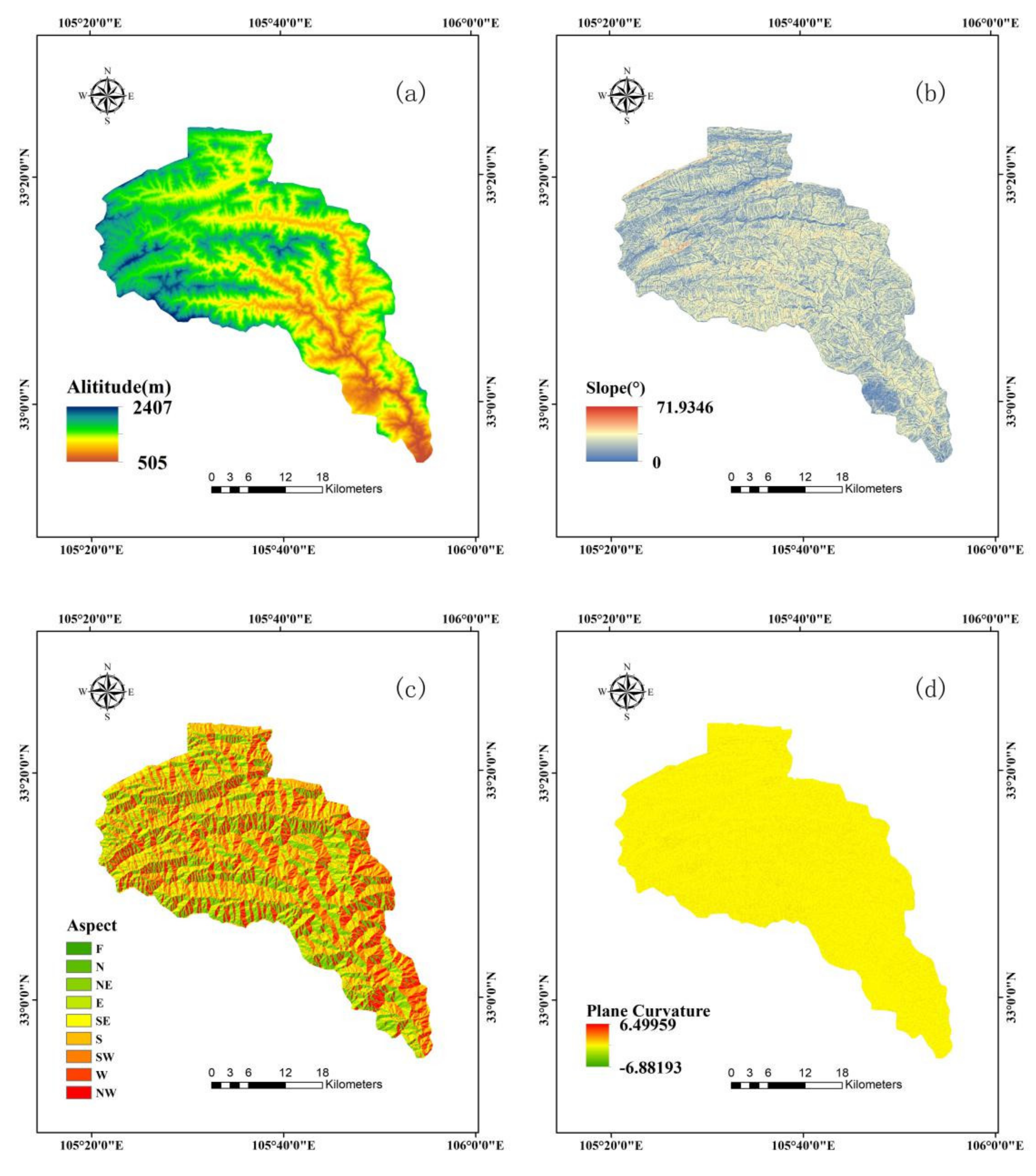
The conditioning factor is a parameter that describes the environment in which complex geological disasters occur. It is inconclusive how to choose the factors in the assessment of susceptibility to geological disasters [2]. Combining previous research and the conditions of the research area, 11 conditioning factors were selected for research in this paper. The conditioning factors were divided as follows: (1) topographic factors, (2) ground conditions, and (3) distance related factors.
The topographic factors (Figure 2a–f) used in this paper, including altitude, slope, aspect, plane curvature, profile curvature, and topographic wetness index (TWI), were mainly produced from a digital elevation model (DEM) with a resolution of 30 m from the Geospatial Data Cloud (http://www.gscloud.cn). The ArcGIS 10.2 software was used for data processing. Altitude affects the temperature, vegetation, land use, and other conditions of an area, so it has a very clear impact on the generation of geological hazards. It is often used in the process of geological hazard susceptibility mapping recently [30]. Since the altitude in the study area has a wide range of fluctuations from 505 m to 2407 m, the altitude could play an important role in the prediction of geological hazards concentrated in a certain altitude range. The slope can effectively reflect the steepness of the study area, and the steep slope is always prone to geological hazards [31]. The slope conditioning factor is, therefore, capable of distinguishing geological hazard samples with steeper slopes from non-geological hazard samples with gentle slopes. The correlation between aspect and geological disasters is mainly that it directly affects the rainfall and sunlight radiation on the slope. A certain aspect of an area may be affected by greater rainfall and weathering, and these areas are usually high-incidence areas of geological hazards. The aspect was widely used in the study of geological hazard susceptibility mapping [32]. The complexity of the terrain was determined by a plane curvature and profile curvature [33], which can affect the generation and development of geological hazards. The TWI takes into account the influence of topography and soil characteristics on the distribution of soil moisture [34]. It quantifies the impact of topography on hydrological activities. TWI is clearly an important conditioning factor in the study area with abundant surface water systems.
In this paper, ground condition factors (Figure 2g–h) include lithology and normalized difference vegetation index (NDVI). The NDVI and lithology were derived from Landsat4-5 TM satellite images with a resolution of 30 m and a geological map at a scale of 1:50,000, respectively. The occurrence of geological hazards can usually be regarded as the process of rock and soil loss of stability. Fragile and susceptible to weathering lithology is usually one of the conditions for the formation of geological hazards. Clearly, most of the geological hazards in this study area are concentrated in the metamorphic rock areas where phyllite and schist are exposed, which makes lithology an important conditioning factor for the following research. NDVI is an important parameter to describe vegetation coverage. Vegetation coverage can affect the stability of rock and soil. In some cases, improving vegetation coverage can effectively reduce the impact of geological hazards. The clear difference in vegetation coverage between geological hazard-prone areas and non-geological hazard-prone areas makes NDVI another important conditioning factor.
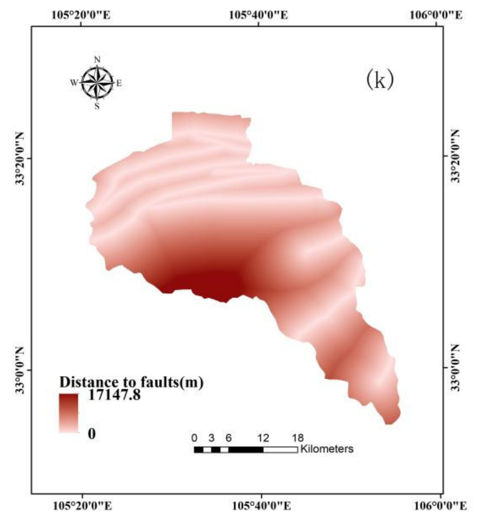
The distance related factors (Figure 2i–k) use distance analysis tools to calculate the distance between a sample and a specific target to evaluate the degree of influence of the target on that sample. Previous studies have shown that the erosion of rivers, human engineering activities, and tectonic activities have an important impact on the formation of geological hazards in the study area [27]. The distance to rivers, the distance to roads, and the distance to faults were, therefore, considered in this paper. The rivers and roads were obtained based on Google Earth images. The faults were recognized from a geological map at a scale of 1:50,000. Combining Figure 1, Figure 2i–k, it can be seen that: (1) geological hazard samples are distributed in strips near the rivers. (2) The areas near the roads, which represent strong human engineering activities, are prone to geological hazards. (3) The density of geological hazards in the area near the faults is much greater than the density of geological hazards in the area far away from the faults.

3.3. The Information Gain Ratio Method

The information gain method (IGR) is an effective tool to evaluate the predictive ability of factors, and was widely used in susceptibility mapping for geological hazards [35,36]. It is based on information theory and adds a penalty coefficient based on the information gain. By tracking the reduction of information entropy, it could quantify the importance of conditioning factors. The formulas of the IGR method are as follows.
G a i n R a t i o S , A = G a i n S , A / I V A
G a i n S , A = E n t S v = 1 V S V S E n t S v
I V A = v = 1 V S v S log 2 S v S
where Gain(S, A) represents the information gain of the factor, Ent(S) is the overall entropy of the data, S is the entire data set, A is the selected attribute, IV(A) is the fixed value of A, and V is the number of attribute values.

3.4. Training and Validation Datasets

Statistical models for susceptibility prediction establish the relationship between independent and dependent variables with training samples and then verifies the relationship with validation samples [37,38]. With references to previous literature [18], the datasets of the three types of geological hazards were all randomly divided into two groups with a ratio of 70/30 for training and validation purposes.

3.5. The Support Vector Machine Method

The SVM (Figure 3) model is a supervised learning model. By projecting complex non-linear sample indexes into the high-dimensional feature space [39], it transforms the high-dimensional complex classification problem into a linearly separable and easy-to-calculate problem. Kernel functions are used to complete this process. Common kernel functions mainly include linear functions (LF), sigmoid functions (SF), radial basis functions (RBF), and polynomial functions (PF).
L F : κ x , y = x T y + c
S F : κ x , y = tan h ( a x T + c )
R B F : κ x , y = exp ( γ | x y | 2 )
P F : κ x , y = ( a x T y + c ) d
where a, c, and γ are parameters of the kernel functions.
There is no clear consensus on the choice of kernel function. Among the four types of kernel functions, the RBF function has good adaptability for the classification problem of data with complex characteristics, and the function parameters are simpler than other kernel functions, which is convenient for debugging. RBF was, therefore, adopted in this study, and its parameter γ was determined to be 0.01, which can make models obtain strong generalization ability in addition to a good performance in the training dataset. The SVM algorithm was applied by IBM SPSS Modeler 18.0.

3.6. The ROC Curves

The ROC curves have been widely used in recent years for geological susceptibility mapping [40]. The method is simple and intuitive, and the accuracy of the analysis method can be observed through the area under curves (AUC). The ROC curves combine sensitivity and specificity with the graphic method, which can accurately reflect the relationship between the specificity and sensitivity of an analytical method. It is a comprehensive reflection of the accuracy of the test. The results based on the training data can be used to evaluate the accuracy rate of the models and the results based on the validation data can be used to evaluate the prediction rate of the models. In previous studies, the AUC was categorized as poor (0.5–0.6), average (0.6–0.7), good (0.7–0.8), very good (0.8–0.9), and excellent (0.9–1) [41].

3.7. The AHP Method

The AHP is a combination of qualitative and quantitative decision analysis methods, and is often used to solve unstructured and complex decision-making problems [32]. It has been widely used in the assessment of a single geological hazard [42,43], and of multiple hazard [44]. The problem that this paper wants to solve is the determination of the optimal weighting scheme for a variety of geological hazards. Due to the qualitative part of the AHP method, it is difficult to give a definite weighting scheme based on this method. The AHP method was, therefore, used to generate multiple reasonable and reliable weighting schemes for collapse, landslide, and debris flow to provide options for the optimal weighting scheme. The point of the AHP method is to make a reasonable and accurate assessment of the relative importance of the geological hazards. The specific steps are as follows.
(a)
Establishing a hierarchical structure model. In this paper, the purpose of applying the AHP method is to obtain the weights of collapse, landslide, and debris flow. The basic model of an analytic hierarchy was adopted, which can be divided into two layers: the target layer and the criterion layer.
(b)
Definition of comparative importance. It is the qualitative part of the AHP. In order to avoid complicated multi-factor comparisons, AHP compares the factors in pairs to improve the accuracy of the comparison. Satty [45] used a nine-point scale to perform the pair-wise comparison process. The definition of comparative importance was shown in Table 1. Since the research object of this paper is three different geological hazards, at the same time, in order to avoid the weight of a single geological hazard being too large or too small, we selected three adjacent relative importance scales of 1, 2, and 3.
(c)
Establishing the judgement matrix. The formula is as follows.
A = ( a i j ) n × n , a i j > 0 , a i j = 1 a j i
where aij is the ratio of relative importance between two factors, and its value was obtained from Table 1.
(d)
Hierarchical ranking and its consistency check. The eigenvector corresponding to the largest eigenvalue λmax of the judgment matrix was normalized (The sum of the elements in the vector is 1) and then recorded as W. The element of W is the sorting weight of the relative importance of the element at the same level to the factor of the upper level. This process is called the hierarchical ranking. In order to check whether there are contradictions in the process of defining relative importance, the consistency check process is necessary, and the formula is as follows.
C I = λ m a x n 1
where CI is the consistency index, λmax is the maximum eigenvalue of the judgement matrix A, and n is the order of the judgment matrix.
C R = C I R I
where RI is the average random consistency, and it is associated with the order of the judgement matrix. The value can be obtained from Table 2. CR is the consistency ratio, and it is used in order to avoid the creation of any incidental judgment in the matrix. If CR < 0.1, the judgement matrix has a good consistency with reasonable judgement. Otherwise, the judgement matrix needs to be revised until the consistency test is satisfied [46].

3.8. The FR Method

To find the optimal weighting scheme from the multiple weighting schemes provided by the AHP method, an evaluation method that can compare and rank the importance of collapse, landslide, and debris flow must be established. At the same time, the optimal weighting scheme for collapse, landslide, and debris flow should be determined according to the characteristics of the study area for better applicability. The FR method, which was widely used to establish the relationship between the conditioning factors that characterize the study area and the occurrence of geological hazards [33], was, therefore, applied in this paper. The formula for calculating the frequency ratio of a certain level of a conditioning factor is as follows.
F R = A i / A t o t B i / B t o t
where subscript i indicates the i-th class for each conditioning factors, Ai represents the number of hazard samples included in the i-th class of a conditioning factor, Atot represents the total number of hazard samples in the study area, Bi is the total number of pixels included in the i-th class of a conditioning factor, and Btot is the total number of pixels in the study area. A larger FR value indicates that the grouping value of a conditioning factor is more conducive to the occurrence of corresponding geological hazards. When a certain geological hazard has achieved larger FR values in multiple groups of a conditioning factor, and these groups occupied most of the study area, then, from the perspective of this conditioning factor, this geological hazard should be given greater weight. Through the analysis of all the conditioning factors, the optimal weighting scheme can be obtained.

3.9. The Superimposing Method for Susceptibility Maps

After obtaining the susceptibility maps of collapse, landslide, and debris flow and the weighting schemes based on the AHP method, the further multiple geological hazard susceptibility maps could be carried out. The major difficulty in a synthesized map is the distinct reference units of all those different hazards. One way to overcome this problem is the classification of single hazard maps, and the multiple geological hazard susceptibility map would be derived by superimposing the classification maps of all the geological hazards [47]. In this paper, the probabilities of all the single geological hazard susceptibility maps were divided into five groups and assigned scores for subsequent summing up. The divided groups were named very low, low, moderate, high, and very high. The scoring standard table was shown in Table 3. Clearly, the process of summing up multiple single geological hazard classification maps was based on the weighting schemes provided by the AHP method.
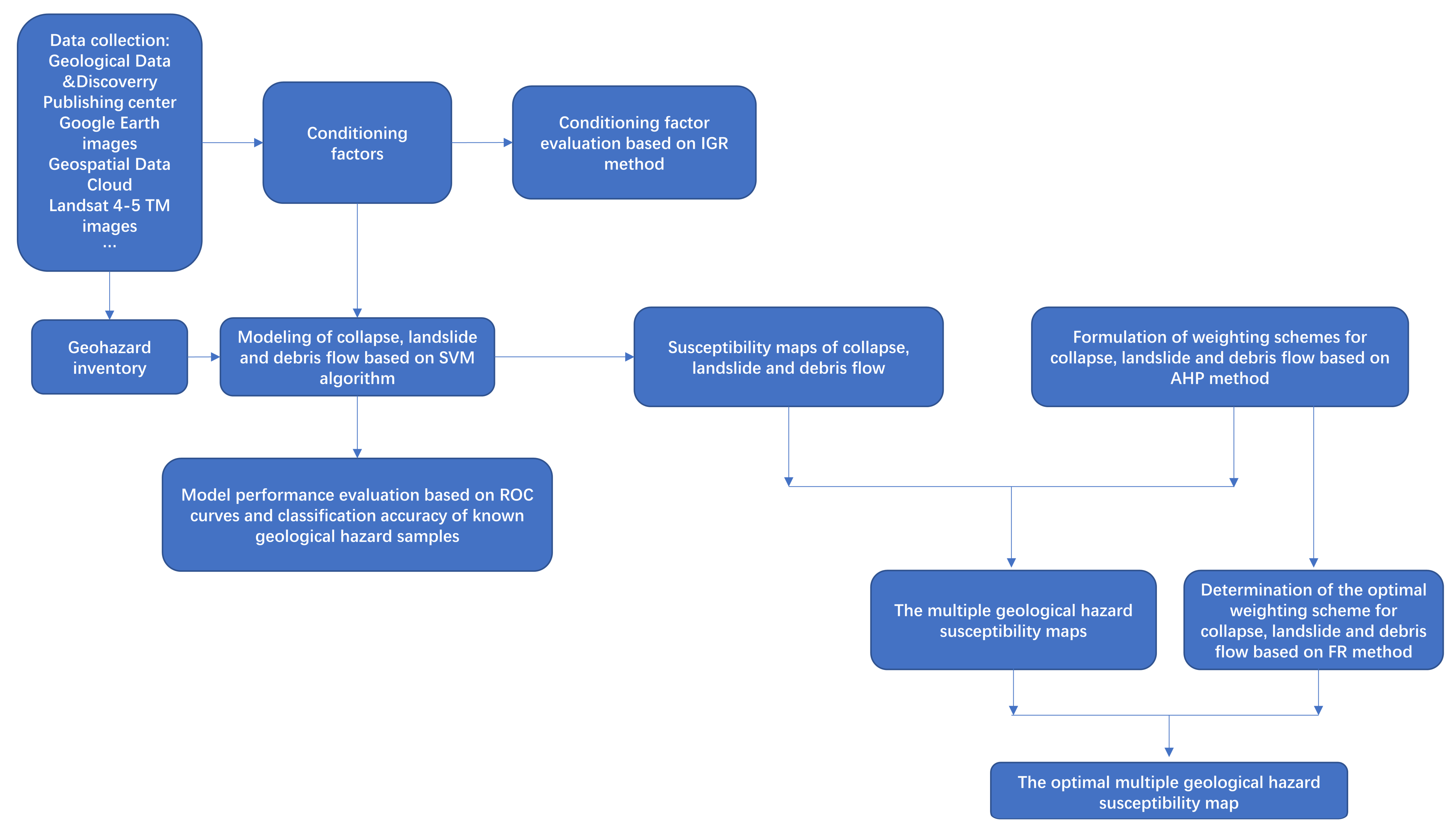
The flowchart showing the methodology used in this study was shown in Figure 4.

4. Results

4.1. The IGR Method Results

In this paper, the IGR method was used for the analysis of the predictive ability of conditioning factors. The results were shown in Figure 5. In general, all the conditioning factors have shown varying degrees of predictive ability for the three types of geological hazards (IGR > 0). The conditioning factors of lithology and distance to roads made the greatest contribution to the prediction of both collapse and landslide while the most important conditioning factors for debris flow are altitude and distance to roads. Considering the conditioning factors as a whole, it can be found that the conditioning factors of debris flow had the strongest predictive ability, while the conditioning factors of landslide showed the worst performance.

4.2. The Basic Geological Hazard Susceptibility Maps

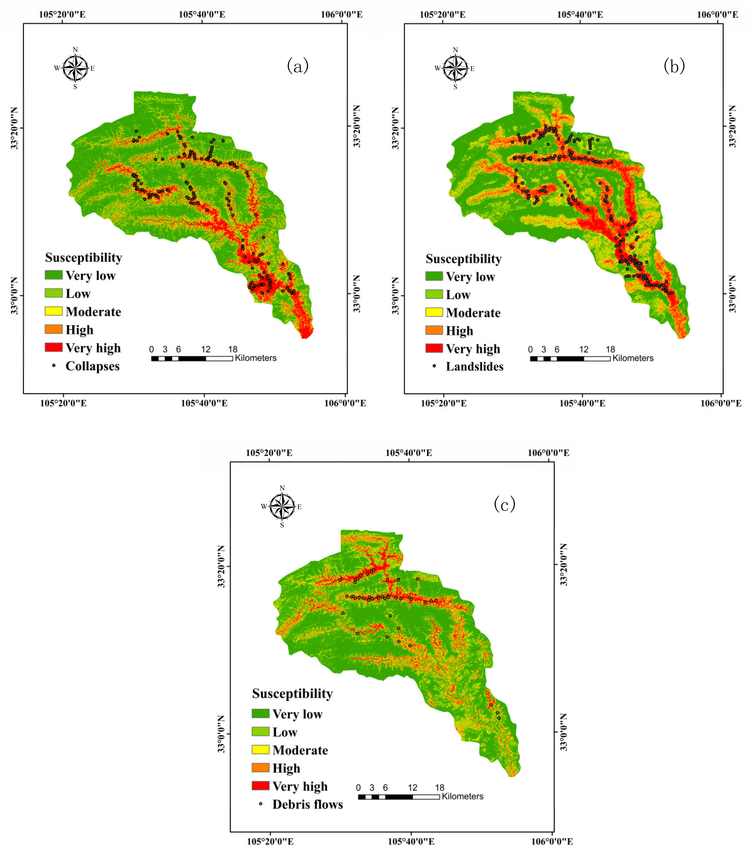
The susceptibility maps of collapse, landslide, and debris flow were shown in Figure 6. In order to test the classification accuracy of the susceptibility map, the grouping values of the samples of collapse, landslide, and debris flow on the corresponding susceptibility maps were counted. The results were shown in Table 4. The results turned out that only a few samples of geological hazards were incorrectly classified. In total, 90.8% of the collapse samples, 91.8% of the landslide samples, and 95.5% of the debris flow samples were classified as moderate or above.

4.3. Assessment of the Model Performance Using ROC Curves

The ROC curves and AUC values using training data were shown in Figure 7. In addition, the results using validation data were shown in Figure 8. For the research on the susceptibility mapping of regional geological hazards, generalization ability is usually one of the most concerned indicators. In this paper, the AUC values obtained based on the validation data were used as an effective tool to test the generalization ability of the models. The results showed that all the models have achieved very good performance on the validation data (0.8 < AUC < 0.9), showing a strong generalization ability. Comparing the three models, on the validation data, the collapse model and the debris flow model behaved similarly, while the landslide model showed a slightly worse performance.

4.4. The Weighting Schemes

In this paper, the weighting schemes for collapse, landslide, and debris flow were obtained based on the AHP method. Based on the selected relative importance scale of 1 to 3, the corresponding judgment matrix can be established. In all the possible judgment matrices, in order to avoid the weight of a single geological hazard being too large or too small, the relative importance combinations 1, 1, 3 and 1, 3, 3 are not in our consideration. According to the remaining relative importance combinations, four different judgment matrices were established. The judgment matrices were shown in Table 5 and the CR values in Table 6 indicate that all the judgment matrices passed the consistency test (CR < 0.1). Since the AHP method itself cannot compare and rank the importance of collapse, landslide, and debris flow, after a series of permutations and combinations, a total of 13 weighting schemes have been proposed (Table 6). The weighting schemes a-f were obtained based on the judgment matrix A1. The weighting scheme g-i correspond to the judgment matrix A2. The weighting scheme j-l were derived from the judgment matrix A3. The weighting scheme m is the product of the judgment matrix A4. The 13 weighting schemes shown in Table 6 correspond to the following four situations: (1) The importance of the three geological hazards was all different. (2) Two of the three geological hazards were of the same importance, and the remaining one was more important. (3) Two of the three geological hazards had the same importance, and the remaining one was less important. (4) The importance of the three geological hazards was all the same. The weighting schemes avoided the over-concentration of weight. For a single geological hazard, the maximum possible weight is 0.539 and the minimum possible weight is 0.164.

4.5. The Multiple Geological Hazard Susceptibility Maps

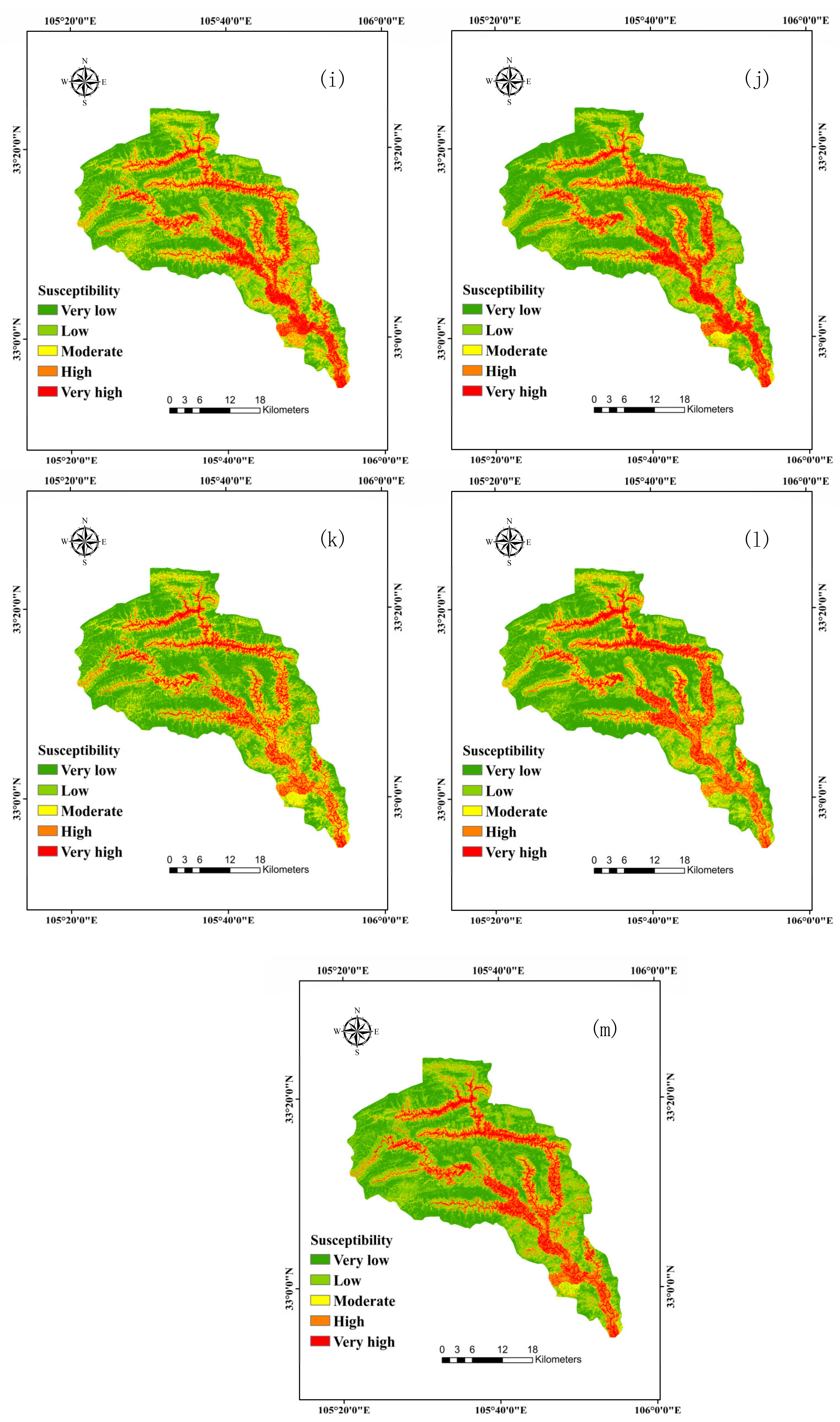
In order to facilitate the use of known geohazard samples to evaluate the quality of multiple geohazard susceptibility maps, the multiple geological hazard susceptibility maps were divided into five groups like the basic geological hazard susceptibility maps, named very low, low, moderate, high, and very high. The multiple susceptibility maps were shown in Figure 9. The proportions of areas with different susceptibility corresponding to the thirteen weighting schemes were shown in Table 7. The results turned out that areas classified as very high or high were all concentrated near the Yanzi River. As for the proportion of areas with different susceptibilities, most of the areas were classified as very low or low, and only a small part of the areas was classified as very high or high.
In this paper, the FR method was used to determine the optimal weighting scheme. The spatial relationship between each geological hazard and conditioning factors was shown in Table 8. The frequency ratios of collapse, landslide, and debris flow were shown in Table 9. For the conditioning factor altitude, at the level of 1300–1600 m and the level of 1600–1900 m, which occupies 58.8% of the entire study area, the frequency ratio of landslides is higher than that of collapse. At the level of <1000 m, 1300–1600 m, 1600–1900 m, and >1900 m, which occupies 78.2% of the entire study area, the frequency ratio of collapse is greater than or equal to that of debris flow. It can be concluded that, from the perspective of altitude, most of the entire study area were most conducive to the occurrence of the landslide, followed by collapse, and the least conducive to the occurrence of debris flows. For the five conditioning factors including slope, plane curvature, profile curvature, NDVI, and distance to the rivers, the same conclusion could be drawn. For the conditioning factor aspect, the predominant sequence of these three geological hazards in the study area is collapse, debris flow, and landslide. For the two conditioning factors of lithology and distance to the roads, most of the study area was most conducive to the occurrence of collapse, followed by the landslide, and the least conducive to the occurrence of debris flow. As for the conditioning factors of TWI and distance to the faults, the occurrence of debris flow has the greatest advantage in most of the study area, followed by the landslide. The occurrence of collapse is not dominant in most of the study area. Comparing the three types of geological hazards in pairs, under 8 of the 11 conditioning factors, landslide occupied a favorable position relative to collapse in most of the entire study area. At the same time, under 9 of 11 conditioning factors, collapse was more likely to occur in most of the entire study area than debris flow. Therefore, the landslide should be given the greatest weight, followed by collapse, and debris flow should be given the least weight. The weighting scheme d in Table 6 is the optimal weighting scheme for this study area.
Based on the optimal weighting scheme, the corresponding multiple geological hazard susceptibility map was determined. All known geological hazard samples were counted to evaluate this susceptibility map. The grouping values of samples of collapse, landslide, and debris flow on the optimal geological hazard susceptibility map were shown in Table 10. The results turned out that only a few samples of geological hazards were incorrectly classified. In total, 92.3% of the collapse samples, 90.1% of the landslide samples, and 95.5% of the debris flow samples were classified as moderate or above. In conclusion, the multiple geological hazard susceptibility maps corresponding to the optimal weighting scheme achieved high-accuracy classification of collapse, landslide, and debris flow samples, which further verified the reliability of the weight determination method proposed in this paper.

5. Discussion

5.1. Evaluation of Conditioning Factors

The evaluation of conditioning factors is very important in the study of geological hazard susceptibility mapping [5]. The IGR method was used to evaluate the predictive ability of conditional factors. Previous studies have shown that conditioning factors with strong predictive ability are usually closely related to the formation of geological hazards [48]. The conditioning factors lithology and distance to roads played an important role in the prediction of both collapses and landslides, indicating the similar formation mechanism of collapse and landslide. (1) Broken and soft metamorphic rocks caused instability in areas prone to collapse and landslides. (2) Frequent human activities near the roads caused the rock and soil to lose stability. For debris flow, the conditioning factor altitude appears to have the greatest contribution, showing the importance of topography for the formation of debris flow. As shown in Table 8, the debris flow samples are mostly concentrated in the low altitude group of 1000-1300 m, and the low altitude may be related to the valley slope topography formed by river erosion [18].
According to the formula of the IGR method, the greater the difference between the samples of a certain geological hazard and the samples of non-geological hazards, the stronger the predictive ability of the conditioning factors of such geological hazards. The result indicates that the conditioning factors of debris flow have the strongest predictive ability, that is, areas prone to debris flow and the non-geological hazard areas showed the biggest difference, which is in good agreement with the FR method result that debris flows are the least prone to occur in most of the study area since the non-geological hazard areas can represent most of the study area well. On the contrary, the result that conditioning factors of landslide showed the weakest predictive ability can also fit the FR result that landslides are the most prone geological hazards in most of the entire study area well.

5.2. Evaluation of the Model Performance

In previous studies, the AUC value on the validation data is often the only indicator to evaluate a model [15]. However, the AUC value is only a reflection of the correct rate of model classification, and it is impossible to evaluate the model’s prediction results in detail. In this paper, the AUC value difference between the collapse model and the debris flow model is very small, so it is difficult to tell which model is better. The classification statistics table of the known samples was, thus, introduced. As shown in Table 4, when compared with the collapse model, the debris flow model can predict a higher proportion of geological hazard samples as high or very high, showing better model performance. The landslide model is the worst-performing model whether from the AUC value or from the sample classification statistics table.
Comparing the results of the IGR method and the performance of the models, it can be found that the stronger the predictive ability of the conditioning factors is, the better the model performance is, showing the importance of high-quality input data for machine learning models.

5.3. Determination of the Optimal Weighting Scheme

It is very important to conduct a comprehensive susceptibility assessment in areas prone to multiple geological hazards. Sun et al. [25] combined four single geological hazard susceptibility maps based on the barrel principle to achieve a comprehensive assessment. Using this method, the comprehensive map will not miss any high susceptibility areas. However, this method cannot distinguish differences in some situations. For example, an area with high susceptibility to only one type of geological hazard and an area with high susceptibility to multiple geological hazards will show the same results on a comprehensive map. In general, this method effectively avoids the underestimation of high-risk areas, but also reduces the accuracy of the comprehensive map. Bathrellos et al. [26] superimposed three single geological hazard susceptibility maps based on a weighting scheme obtained by the AHP method. However, the AHP method has some clear limitations. One of the most important problems is the uncertainty of this method, which may happen from selection, comparison, and ranking of multiple factors [49]. In this paper, the FR method was used to solve the main limitation and further obtain the optimal weighting scheme. Through the analysis of the FR method, the predominant sequence of collapse, landslide, and debris flow that are applicable in most of the entire study areas can be obtained. It can be seen that the FR method can complete the multi-factor comparison and ranking process based on objective data, which effectively reduced the uncertainty of the AHP method. The results showed that this method of determining the optimal weight scheme is very effective. As shown in Table 10, the multiple geological hazard susceptibility map based on the optimal weighting scheme realized high-accuracy classification of all geological hazard samples, showing the high quality of this multiple geological hazard susceptibility map.

5.4. Limitations

In this paper, there are mainly the following limitations. (1) The susceptibility to geological hazards was obtained based on the SVM algorithm. Different geological hazard susceptibility algorithms usually perform differently, so more algorithms should be used for research to improve the quality of the susceptibility assessment to geological hazards. (2) The determination of the optimal weighting scheme is a complicated process, so more factors could be considered to determine the optimal weighting scheme.

6. Conclusions

The purpose of this paper is to establish a method for determining the optimal weighting scheme for multiple geological hazard susceptibility mapping. First, the IGR method was used to evaluate the model performance and the SVM algorithm was applied to obtain the susceptibility maps of collapse, landslide, and debris flow. Subsequently, the ROC method and the prediction results of the known geohazard samples were used to evaluate the performance of the models. Then the AHP method was used to generate possible and reasonable weighting schemes. Finally, the FR method was used to determine the optimal weighting scheme. It was found that: (1) the predictive ability of the conditioning factors of different geological hazards showed that human activities and broken metamorphic rocks played an important role in the formation of collapses and landslides, while the valley slope topography associated with low altitude contributed the most to the formation and development of debris flow in this study area. It was also found that: (2) the performance of machine learning models highly depends on the quality of the input data. The stronger the predictive ability of the conditioning factors, the better the model performance. Lastly, it was discovered that: (3) by introducing the FR method to reduce the uncertainty of the AHP method, an optimal weighting scheme that can produce high-quality multiple geological hazard susceptibility maps can be obtained. The conclusions in this paper could provide a meaningful reference for the study of susceptibility in areas where a variety of geological hazards develop.

Author Contributions

Conceptualization, Ruiyuan Gao. Data curation, Bailong Li. Formal analysis, Changming Wang and Songling Han. Funding acquisition, Changming Wang. Investigation, Songling Han. Methodology, Ruiyuan Gao, Zhu Liang, and Bailong Li. Project administration, Changming Wang. Resources, Zhu Liang and Bailong Li. Visualization, Songling Han. Writing—original draft, Ruiyuan Gao. Writing—review & editing, Ruiyuan Gao and Zhu Liang. All authors have read and agreed to the published version of the manuscript.

Funding

This research was funded by the National Natural Science Foundation of China (Grant No.41972267) and Graduate Innovation Fund of Jilin University.

Data Availability Statement

The test data used to support the findings of this study are provided by the Geoscientific Data & Discovery Publishing System and Geospatial Data Cloud.

Acknowledgments

The authors of this article are grateful for the National Natural Science Foundation of China (Grant No.41972267) and Graduate Innovation Fund of Jilin University.

Conflicts of Interest

The authors declare no conflict of interest.

References

  1. Wang, J.J.; Yin, K.L.; Xiao, L.L. Landslide susceptibility assessment based on GIS and weighted information value: A case study of Wanzhou district, three gorges reservoir. Chin. J. Rock Mech. Eng. 2014, 33, 797–808. [Google Scholar] [CrossRef]
  2. Reichenbach, P.; Rossi, M.; Malamud, B.; Mihir, M.; Guzzetti, F. A review of statistically-based landslide susceptibility models. Earth Sci. Rev. 2018, 180, 60–91. [Google Scholar] [CrossRef]
  3. Corominas, J.; van Westen, C.; Frattini, P.; Casini, L.; Malet, J.-P.; Fotopoulou, S.; Catani, F.; Van Den Eeckhaut, M.; Mavrouli, O.; Agliardi, F.; et al. Recommendations for the quantitative analysis of landslide risk. Bull. Eng. Geol. Environ. 2014, 73, 209–263. [Google Scholar] [CrossRef]
  4. Yao, X.; Tham, L.G.; Dai, F.C. Landslide susceptibility mapping based on support vector machine: A case study on natural slopes of Hong Kong, China. Geomorphology. 2008, 101, 572–582. [Google Scholar] [CrossRef]
  5. Chang, K.T.; Merghadi, A.; Yunus, A.P.; Pham, B.T.; Dou, J. Evaluating scale effects of topographic variables in landslide susceptibility models using GIS-based machine learning techniques. Sci. Rep. 2019, 9, 12296. [Google Scholar] [CrossRef] [Green Version]
  6. Nguyen, M.D.; Pham, B.T.; Tuyen, T.; Yen, H.P.H.; Prakash, I.; Thanh, T.V.; Chapi, K.; Shirzadi, A.; Shahabi, H.; Dou, J.; et al. Development of an Artificial Intelligence Approach for Prediction of Consolidation Coefficient of Soft Soil: A Sensitivity Analysis. Open Constr. Build. Technol. 2019, 13. [Google Scholar] [CrossRef]
  7. Pham, B.T.; Prakash, I.; Dou, J.; Singh, S.K.; Trinh, P.T.; Tran, H.T.; Le, T.M.; Van, P.T.; Khoi, D.K.; Shirzadi, A.; et al. A novel hybrid approach of landslide susceptibility modelling using rotation forest ensemble and different base classifiers. Geocarto Int. 2019, 35, 1–25. [Google Scholar] [CrossRef]
  8. Tien, B.D.; Shirzadi, A.; Shahabi, H.; Geertsema, M.; Omidvar, E.; Clague, J.J.; Thai Pham, B.; Dou, J.; Talebpour, A.D.; Bin Ahmad, B.; et al. New Ensemble Models for Shallow Landslide Susceptibility Modeling in a Semi-Arid Watershed. Forests 2019, 10, 743. [Google Scholar] [CrossRef] [Green Version]
  9. Bergstra, J.; Yamins, D.; Cox, D.D. Making a Science of Model Search: Hyperparameter Optimization in Hundreds of Dimensions for Vision Architectures. In Proceedings of the 30th International Conference on Machine Learning, Atlanta, GE, USA, 16–21 June 2013. [Google Scholar]
  10. Khosravi, K.; Shahabi, H.; Pham, B.T.; Adamowski, J.; Shirzadi, A.; Pradhan, B.; Dou, J.; Ly, H.B.; Gróf, G.; Ho, H.L.; et al. A comparative assessment of flood susceptibility modeling using Multi-Criteria Decision-Making Analysis and Machine Learning Methods. J. Hydrol. 2019, 573, 311–323. [Google Scholar] [CrossRef]
  11. Pham, B.T.; Shirzadi, A.; Tien, B.D.; Prakash, I.; Dholakia, M.B. A hybrid machine learning ensemble approach based on a radial basis function neural network and rotation forest for landslide susceptibility modeling: A case study in the Himalayan area, India. Int. J. Sediment Res. 2018, 33, 157–170. [Google Scholar] [CrossRef]
  12. Chen, W.; Xie, X.; Peng, J.; Wang, J.; Duan, Z.; Hong, H. GIS-based landslide susceptibility modelling: A comparative assessment of kernel logistic regression, Naive-Bayes tree, and alternating decision tree models. Geomat. Nat. Haz. Risk 2017, 8, 950–973. [Google Scholar] [CrossRef] [Green Version]
  13. Wang, L.J.; Guo, M.; Sawada, K.; Lin, J.; Zhang, J. A comparative study of landslide susceptibility maps using logistic regression, frequency ratio, decision tree, weights of evidence and artificial neural network. Geosci. J. 2016, 20, 117–136. [Google Scholar] [CrossRef]
  14. Hong, H.; Pradhan, B.; Neamah Jebur, M.; Tien Bui, D.; Xu, C.; Akgun, A. Spatial prediction of landslide hazard at the Luxi area (China) using support vector machines. Environ. Earth Sci. 2016, 75, 40. [Google Scholar] [CrossRef]
  15. Liang, Z.; Wang, C.M.; Han, S.L.; Kaleem, U.J.K.; Liu, Y.A. Classification and susceptibility assessment of debris flow based on a semi-quantitative method combination of the fuzzy C-means algorithm, factor analysis and efficacy coefficient. Nat. Hazards Earth Syst. Sci. 2020, 20, 1287–1304. [Google Scholar] [CrossRef]
  16. Oh, H.J.; Lee, S. Shallow Landslide Susceptibility Modeling Using the Data Mining Models Artificial Neural Network and Boosted Tree. Appl. Sci. 2017, 7. [Google Scholar] [CrossRef] [Green Version]
  17. Pham, B.T.; Nguyen-Thoi, T.; Qi, C.C.; Phong, T.V.; Dou, J.; Lanh, S.H.; Hiep, V.L.; Prakash, I. Coupling RBF neural network with ensemble learning techniques for landslide susceptibility mapping. Catena 2020, 195, 104805. [Google Scholar] [CrossRef]
  18. Merghadi, A.; Yunus, A.P.; Dou, J.; Whiteley, J.; Thai, P.B.; Bui, D.T.; Avtar, R.; Abderrahmane, B. Machine learning methods for landslide susceptibility studies: A comparative overview of algorithm performance. Earth Sci. Rev. 2020, 207, 103225. [Google Scholar] [CrossRef]
  19. Gruber, F.E.; Mergili, M. Regional-scale analysis of high-mountain multi-hazard and risk indicators in the Pamir (Tajikistan) with GRASS GIS. Nat. Hazards Earth Syst. Sci. 2013, 13, 2779–2796. [Google Scholar] [CrossRef] [Green Version]
  20. Marzocchi, W.; Garcia-Aristizabal, A.; Gasparini, P.; Mastellone, M.L.; Di, R.A. Basic principles of multi-risk assessment: A case study in Italy. Nat. Hazards. 2012, 62, 551–573. [Google Scholar] [CrossRef]
  21. Tate, E.; Cutter, S.L.; Berry, M. Integrated multihazard mapping. Environ. Plann. B Plann. Des. 2010, 37, 646–663. [Google Scholar] [CrossRef] [Green Version]
  22. Gallina, V.; Torresan, S.; Critto, A.; Sperotto, A.; Glade, T.; Marcomini, A. A review of multirisk methodologies for natural hazards: Consequences and challenges for a climate change impact assessment. J. Environ. Manag. 2016, 168, 123–132. [Google Scholar] [CrossRef]
  23. Carpignano, A.; Golia, E.; Di, M.C.; Bouchon, S.; Nordvik, J.P. A methodological approach for the definition of multi-risk maps at regional level: First application. J. Risk Res. 2009, 12, 513–534. [Google Scholar] [CrossRef]
  24. Zhang, L.; Zhang, S. Approaches to multi-hazard landslide risk assessment. In Proceedings of the Geo-risk Conference, Denver, CO, USA, 4–7 June 2017. [Google Scholar]
  25. Sun, L.; Ma, C.; Li, Y. Multiple geo-environmental hazards susceptibility assessment: A case study in Luoning County, Henan Province, China. Geomat. Nat. Hazards Risk. 2019, 10, 2009–2029. [Google Scholar] [CrossRef]
  26. Bathrellos, G.D.; Skilodimou, H.D.; Chousianitis, K.; Youssef, A.M.; Pradhan, B. Suitability estimation for urban development using multi-hazard assessment map. Sci. Total Environ. 2017, 575, 119–134. [Google Scholar] [CrossRef]
  27. Ye, Z.N.; Yang, Q.; Li, Q.; Zhang, X.H. Landslide characteristics and hazard assessment in Yanzi River Basin. J. Liaoning Tech. Univ. (Nat. Sci.) 2020, 39, 145–151. [Google Scholar] [CrossRef]
  28. Yang, Q.; YE, Z.N.; Gao, Y.L.; Li, Q.; Ding, W.C. Dataset of the 2015 Geo-Hazard Survey of the Yanzi River Basin, Upstream of the Jialing River. Geol. China. 2018, 45, 156–167. [Google Scholar]
  29. Yang, Q.; Wang, S.Y.; Ye, Z.N. Analysis on the development of geological hazard and failure mode in Yanzi River Basin. J. Eng. Geol. 2019, 27, 289–295. [Google Scholar] [CrossRef]
  30. Pradhan, A.M.S.; Kim, Y.T. Relative effect method of landslide susceptibility zonation in weathered granite soil: A case study in Deokjeok-ri Creek, South Korea. Nat. Hazards 2014, 72, 1189–1217. [Google Scholar] [CrossRef]
  31. Varnes, D.J. Landslide Hazard Zonation: A Review of Principles and Practice; United Nations: Paris, France, 1984; p. 63. [Google Scholar]
  32. Pourghasemi, H.R.; Mohammady, M.; Pradhan, B. Landslide susceptibility mapping using index of entropy and conditional probability models in GIS: Safarood Basin, Iran. Catena 2012, 97, 71–84. [Google Scholar] [CrossRef]
  33. Oh, H.J.; Pradhan, B. Application of a neuro-fuzzy model to landslide-susceptibility mapping for shallow landslides in a tropical hilly area. Comput. Geosci. 2011, 37, 1264–1276. [Google Scholar] [CrossRef]
  34. Pourghasemi, H.R.; Jirandeh, A.G.; Pradhan, B.; Xu, C.; Gokceoglu, C. Landslide susceptibility mapping using support vector machine and GIS at the Golestan Province, Iran. J. Earth Syst. Sci. 2013, 122, 349–369. [Google Scholar] [CrossRef] [Green Version]
  35. Bui, D.T.; Ho, T.C.; Pradhan, B.; Pham, B.T.; Nhu, V.H.; Revhaug, I. GIS-based modeling of rainfall-induced landslides using data mining-based functional trees classifier with AdaBoost, Bagging, and MultiBoost ensemble frameworks. Environ. Earth Sci. 2016, 75, 22. [Google Scholar] [CrossRef]
  36. Dou, J.; Yunus, A.P.; Bui, D.T.; Merghadi, A.; Sahana, M.; Zhu, Z.F.; Chen, C.W.; Han, Z.; Pham, B.T. Improved landslide assessment using support vector machine with bagging, boosting, and stacking ensemble machine learning framework in a mountainous watershed, Japan. Landslides 2020, 17, 641–658. [Google Scholar] [CrossRef]
  37. Guzzetti, F.; Reichenbach, P.; Ardizzone, F.; Cardinali, M.; Galli, M. Estimating the quality of landslide susceptibility models. Geomorphology 2006, 81, 166–184. [Google Scholar] [CrossRef]
  38. Guzzetti, F.; Galli, M.; Reichenbach, P.; Ardizzone, F.; Cardinali, M. Landslide hazard assessment in the Collazzone area, Umbria, central Italy. Nat. Hazard. Earth Syst. Sci. 2006, 6, 115–131. [Google Scholar] [CrossRef]
  39. Xu, C.; Dai, F.; Xu, X.; Lee, Y.H. GIS-based support vector machine modeling of earthquake-triggered landslide susceptibility in the Jianjiang River watershed, China. Geomorphology 2012, 145, 70–80. [Google Scholar] [CrossRef]
  40. Provost, F.; Fawcett, T. Robust classification for imprecise environments. Mach. Learn. 2001, 42, 203–231. [Google Scholar] [CrossRef]
  41. Chen, W.; Pourghasemi, H.R.; Naghibi, S.A. A comparative study of landslide susceptibility maps produced using support vector machine with different kernel functions and entropy data mining models in China. Bull. Eng. Geol. Environ. 2018, 77, 647–664. [Google Scholar] [CrossRef]
  42. Karaman, H.; Erden, T. Net earthquake hazard and elements at risk (NEaR) map creation for city of Istanbul via spatial multi-criteria decision analysis. Nat. Hazards 2014, 73, 685–709. [Google Scholar] [CrossRef]
  43. Rozos, D.; Bathrellos, G.D.; Skilodimou, H.D. Comparison of the implementation of rock engineering system (RES) and analytic hierarchy process (AHP) methods, based on landslide susceptibility maps, compiled in GIS environment. A case study from the eastern Achaia County of Peloponnesus, Greece. Environ. Earth Sci. 2011, 63, 49–63. [Google Scholar] [CrossRef]
  44. Peng, S.H.; Shieh, M.J.; Fan, S.Y. Potential hazard map for disaster prevention using GIS-based linear combination approach and analytic hierarchy method. J. Geogr. Inf. Syst. 2012, 4, 403–411. [Google Scholar] [CrossRef] [Green Version]
  45. Saaty, T.L. A scaling method for priorities in hierarchical structures. Math. Psychol. 1977, 15, 234–281. [Google Scholar] [CrossRef]
  46. Saaty, T.L. How to make a decision: The analytic hierarchy process. Eur. J. Oper. Res. 1990, 48, 9–26. [Google Scholar] [CrossRef]
  47. Delmonaco, G.; Margottini, C.; Spizzichino, D. New Methodology for Multi-Risk Assessment and the Harmonisation of Different Natural Risk Maps; Armonia Project: Rome, Italy, 2006. [Google Scholar]
  48. Dai, F.; Lee, C.; Ngai, Y. Landslide risk assessment and management: An overview. Eng. Geol. 2002, 64, 65–87. [Google Scholar] [CrossRef]
  49. Bathrellos, G.D.; Gaki-Papanastassiou, K.; Skilodimou, H.D.; Skianis, G.A.; Chousianitis, K.G. Assessment of rural community and agricultural development using geomorphological–geological factors and GIS in the Trikala prefecture (Central Greece). Stoch. Environ. Res. Risk A 2013, 27, 573–588. [Google Scholar] [CrossRef]
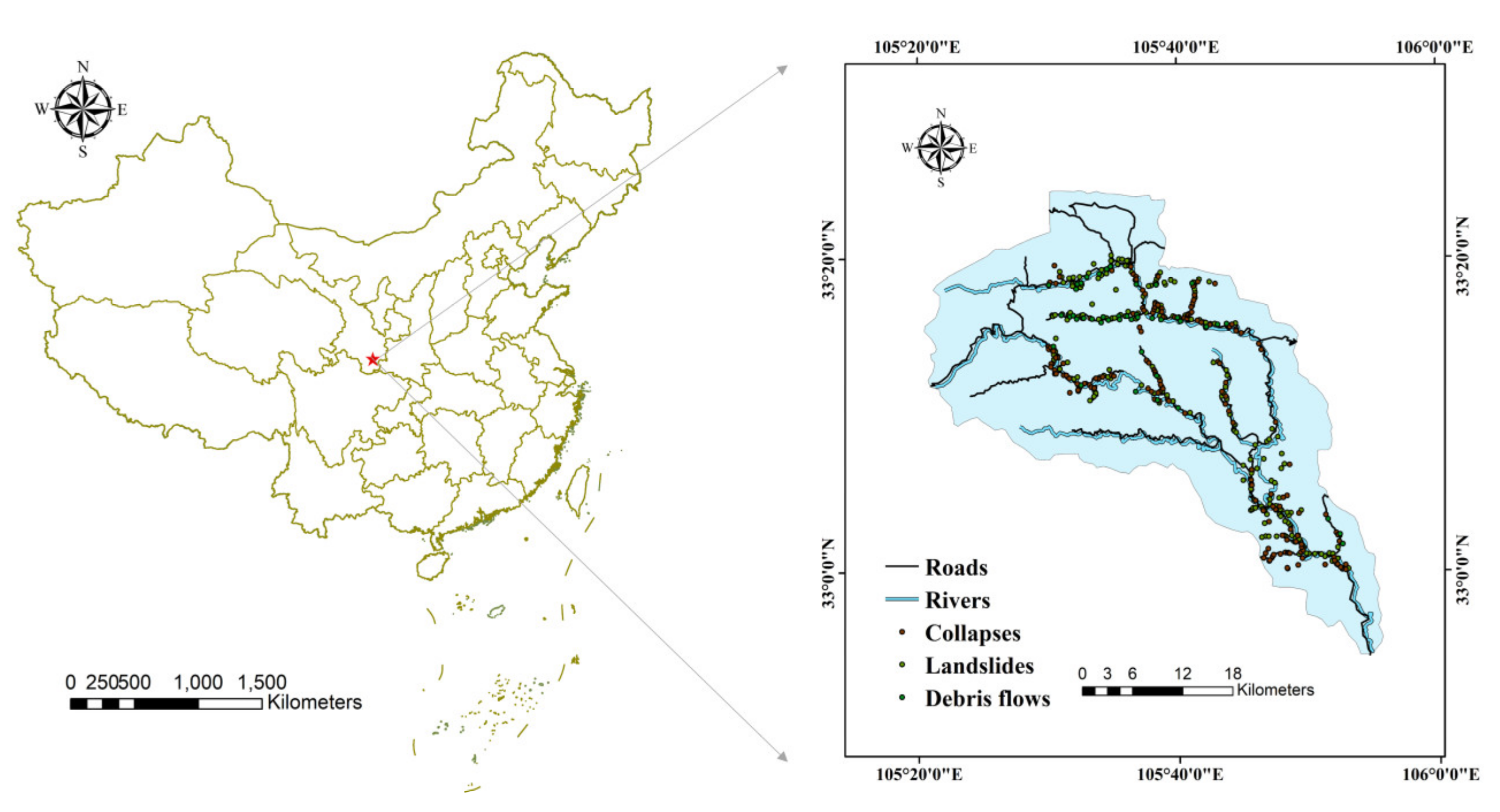
Figure 1. Location of the Yanzi River Basin and the geological hazard distribution map (Source: Dataset of the 2015 Geo-Hazard Survey of the Yanzi River Basin, Upstream of the Jialing River).
Ijgi 10 00218 g001
Figure 2. Conditioning factors: (a) Altitude. (b) Slope. (c) Aspect. (d) Plane curvature. (e) Profile curvature. (f) TWI. (g) NDVI. (h) Lithology. (i) Distance to rivers. (j) Distance to roads. (k) Distance to faults.
Ijgi 10 00218 g002aIjgi 10 00218 g002bIjgi 10 00218 g002c
Figure 3. Schematic diagram of the support vector machine (SVM) method.
Ijgi 10 00218 g003
Figure 4. Flowchart of the methodology used in this study.
Ijgi 10 00218 g004
Figure 5. The information gain ratios of the conditioning factors for collapse, landslide, and debris flow.
Ijgi 10 00218 g005
Figure 6. The basic geological hazard susceptibility maps: (a) Collapse susceptibility map, (b) landslide susceptibility map, and (c) debris flow susceptibility map.
Ijgi 10 00218 g006
Figure 7. The ROC curves based on training data. (a) The ROC curve of collapse. (b) The ROC curve of the landslide. (c)The ROC curve of debris flow.
Ijgi 10 00218 g007
Figure 8. The ROC curves based on validation data: (a) The ROC curve of collapse. (b) The ROC curve of landslide. (c) The ROC curve of debris flow.
Ijgi 10 00218 g008
Figure 9. The multiple geological hazard susceptibility maps: Maps (a)–(m) correspond to weighting schemes a to m.
Ijgi 10 00218 g009aIjgi 10 00218 g009bIjgi 10 00218 g009c
Table 1. Definition of comparative importance.
1Two factors are equally important
3One factor is more important
5One factor is strongly more important
7One factor is very strongly more important
9One factor is extremely more important
2, 4, 6,8 Intermediate values
Table 2. The random average consistency index.
n123456789101112
RI000.520.891.121.261.361.411.461.491.521.54
Table 3. Scoring standard table of geological hazard probability.
Probability LevelScore
Very low1
Low2
Moderate3
High4
Very high5
Table 4. The sample statistical results of the basic susceptibility maps.
GroupsNo. of CollapsesPercentage of CollapsesNo. of LandslidesPercentage of LandslidesNo. of Debris FlowsPercentage of Debris Flows
Very low84.7%115.0%00.0%
Low63.5%73.2%24.5%
Moderate158.8%3013.5%36.8%
High2816.5%4018.0%49.1%
Very high11366.5%13460.3%3579.5%
Table 5. The judgment matrices.
A 1A 2
ElementHazard 1Hazard 2Hazard 3ElementHazard 1Hazard 2Hazard3
Hazard 110.50.33Hazard 1110.5
Hazard 2210.5Hazard 2110.5
Hazard 3321Hazard 3221
A 3A 4
ElementHazard 1Hazard 2Hazard 3ElementHazard 1Hazard 2Hazard3
Hazard 110.50.5Hazard 1111
Hazard 2211Hazard 2111
Hazard 3211Hazard 3111
Table 6. The weighting schemes.
Types of Weighting SchemesWeighting SchemesWeight of CollapseWeight of LandslideWeight of Debris FlowCIRICR
1a0.1640.2970.5390.0050.520.009
b0.1640.5390.297
c0.2970.1640.539
d0.2970.5390.164
e0.5390.1640.297
f0.5390.2970.164
2g0.2500.2500.50000
h0.2500.5000.250
i0.5000.2500.250
3j0.4000.4000.20000
k0.4000.2000.400
l0.2000.4000.400
4m0.3330.3330.33300
Table 7. The classification distribution table of the susceptibility map of geological disasters.
MapsMap 1Map 2Map 3Map 4Map 5Map 6Map 7Map 8Map 9Map 10Map 11Map 12Map 13
Susceptibility
Very low42.0%40.0%42.0%40.0%41.5%41.5%31.4%31.4%31.4%35.4%37.5%35.9%31.4%
Low20.6%23.2%21.0%23.1%23.3%20.6%25.8%24.6%25.6%25.1%24.2%25.0%34.7%
Moderate16.2%13.7%16.1%13.6%14.8%14.2%19.2%17.5%17.7%13.8%17.5%14.0%8.2%
High12.3%12.5%12.2%12.3%12.2%11.7%13.3%13.8%12.8%13.4%11.0%15.1%14.2%
Very high8.8%10.7%8.7%11.1%8.2%12.0%10.3%12.7%12.5%12.3%9.8%10.0%11.5%
Table 8. Spatial relationship between each conditioning factor and geohazard.
FactorsClassNo. of
Landslide
Percentage of LandslideNo. of
Collapse
Percentage of CollapseNo. of
Debris Flow
Percentage of
Debris Flow
Altitude
(m)
<10007935.56136.349.1
1000–13008739.27343.53579.5
1300–16005524.83420.2511.4
1600–190010.50000.0
>1900000000.0
Slope (°)<153314.97242.82556.8
15–247935.63923.21840.9
24–3380363017.912.3
>333013.52716.100.0
AspectFlat000000.0
North198.5116.51022.7
North east3917.64023.9818.2
East2092213.124.5
South east3917.62313.7511.4
South4922.1148.3511.4
Southwest31142514.9715.9
West156.81810.749.1
Northwest104.4158.936.8
Plan curvature<−0.473.2137.7511.4
−0.4–09040.510160.12659.1
0–0.410145.54627.41329.5
>0.42410.884.800.0
Profile curvature<−0.583.65300.0
−0.5–07332.94225613.6
0–0.511953.689533170.5
>0.5229.93219715.9
TWI<57734.72716.136.8
5–79040.56840.51840.9
7–114922.15633.31534.1
>1162.71710.1818.2
Lithology131.331.700.0
24218.91061227.3
311551.810864.300.0
45926.73118.52965.9
531.3169.536.8
NDVI<0.13515.84325.6715.9
0.1–0.23917.647281125.0
0.2–0.36428.85130.41738.6
>0.38437.82716920.5
Distance to rivers (m)<11001627311970.82352.3
1100–24002310.32917.3613.6
2400–37002611.7137.7715.9
>370011574.2818.2
Distance to faults (m)<250012355.47544.73579.5
2500–55005826.14023.836.8
5500–10,0004118.55331.5613.6
>10,000000000.0
Distance to roads (m)<100018884.714586.34090.9
1000–2000115169.524.5
2000–40002095312.3
>400031.321.212.3
Table 9. The frequency ratio of three geological hazards.
FactorsClassNo. of Pixels in DomainPercentage of DomainFrequency Ratio of CollapseFrequency Ratio of LandslideFrequency Ratio of Debris Flow
Altitude (m)<1000166,22011.23.243.170.81
1000–1300324,92721.82.001.803.65
1300–1600503,25633.80.600.730.34
1600–1900387,049260.000.020.00
>1900106,9627.20.000.000.00
Slope (°)<15256,29717.22.490.873.30
15–24474,63831.90.731.121.28
24–33525,26835.30.511.020.07
>33232,21115.61.030.870.00
AspectFlat33550.20.000.000.00
North192,20912.90.500.661.76
North east187,10112.61.901.401.44
East166,74711.21.170.800.40
South east203,54413.71.001.280.83
South223,046150.551.470.76
Southwest186,66312.51.191.121.27
West150,01910.11.060.670.90
Northwest175,73011.80.750.370.58
Plan curvature<−0.4162,33710.90.710.291.05
−0.4–0577,53938.81.551.041.52
0–0.4562,12437.80.721.200.78
>0.4186,41412.50.380.860.00
Profile curvature<−0.5107,4707.20.420.500.00
−0.5–0608,29140.90.610.800.33
0–0.5659,24244.31.201.211.59
>0.5113,4117.62.501.302.09
TWI<5603,10640.50.400.860.17
5–7641,10443.10.940.940.95
7–11207,852142.381.582.44
>1136,3512.44.211.137.58
Lithology149,8463.30.520.390.00
2337,62122.70.260.831.20
3871,76758.61.100.880.00
4179,42012.11.532.215.45
548,6093.32.880.392.06
NDVI<0.1212,37314.31.791.101.11
0.1–0.2249,01616.71.681.051.50
0.2–0.3433,39529.11.040.991.33
>0.3593,63039.90.400.950.51
Distance to rivers (m)<1100505,451342.082.151.54
1100–2400454,05730.50.570.340.45
2400–3700289,40019.40.400.600.82
>3700239,50616.10.260.311.13
Distance to faults (m)<2500748,37650.30.891.101.58
2500–5500370,76124.90.961.050.27
5500–10,000245,78316.51.911.120.82
>10,000123,4948.30.000.000.00
Distance to roads (m)<1000594,05839.92.162.122.28
1000–2000430,80428.90.330.170.16
2000–4000357,265240.130.380.10
>4000106,2877.10.170.180.32
Table 10. The sample statistical results of the multiple susceptibility maps.
GroupsNo. of
Collapses
Percentage of
Collapses
No. of
Landslides
Percentage of LandslidesNo. of
Debris Flows
Percentage of
Debris Flows
Very low42.4%62.7%00.0%
Low95.3%167.2%14.5%
Moderate2011.8%2310.4%76.8%
High3621.2%6428.8%119.1%
Very high10159.4%11350.9%2575.6%
Publisher’s Note: MDPI stays neutral with regard to jurisdictional claims in published maps and institutional affiliations.