Encoding Conversion Algorithm of Quaternary Triangular Mesh

Abstract

In the process of global information construction, different fields have built their own discrete global grid systems (DGGS). With the development of big data technology, data exchange, integration, and update have gradually become a trend, as well as the associative integration of different DGGS. Due to the heterogeneity of DGGS and the different encoding rules, how to build the encoding conversion rules and data mapping relationship between the same object in various DGGS is an effective support and key technology to achieve the interoperability of DGGS. As a kind of multipurpose DGGS, the quaternary triangular mesh (QTM) has become an effective spatial framework for constructing the digital earth because of its simple structure. At present, there are many schemes for QTM encoding research, which plays a key role in the development of QTM, but at the same time, it also leads to difficulties in the communication and integration of QTM under different encoding. In order to solve this problem, we explore the characteristics of QTM encoding, and put forward three conversion algorithms: resampling conversion algorithm, hierarchical conversion algorithm, and row–column conversion algorithm.

1. Introduction

A Discrete global grid system (DGGS) is a suitable grid system for representing the Earth, and it can indefinitely subdivide a sphere without changing its grid shape. Each subdivision level has a regular structure, so there are strict transformation relations between grids at different subdivision levels, which provides a unified expression model for the fusion of geographic data with arbitrary distribution and different scales [1,2,3,4]. In addition, a DGGS is characterized by discrete hierarchy and global continuity. It is not limited by the type of map projection. A DGGS can fundamentally solve problems inherent in planar map projections, such as such as data discontinuities, geometric deformation, scale transformations, and topological inconsistency when handling global spatiotemporal data [5,6].

Quaternary triangular mesh (QTM) is a DGGS based on an inscribed regular octahedron [7]. It has the characteristics of hierarchical organization and continuous sorting [8], and it also conforms to spherical characteristics. In recent years, many scholars have used the QTM structure to explore global spatial data extraction and multi-resolution management [9], spatial data hierarchical indexing [10], map synthesis and fuzzy data discrimination [11,12], and global navigation [13]. However, because various implementations of QTM employ different indexing and encoding schemes, translating data from one to another can be a problem.

The problem of geographic information interoperability has a long history. Like earlier GI frameworks, interoperability of DGGS has become an obstacle to its further development [14]. In 2014, the Open Geospatial Consortium (OGC) established the Global Discrete Grid Standardization Working Group to promote the progress of DGGS interoperability across domains (or disciplines) [1]. Especially after OGC promulgated the DGGS standard in 2017, it strongly advocated this research.

In order to exchange, unify, or standardize the data represented by different forms of the DGGS, Arimi first proposed a categorization of indexing methods used for DGGS and then defined a general process for their interconversion [15]. Lingyu Du found “weak duality" relations between the hexagonal grid and the triangular or rhombus grid and established a unified transformation relationship between heterogeneous grids and vector line grid expression models [16]. Arimi realized an efficient visualization algorithm that was applicable to a variety of hexagonal grids [17]. Jin Ben combined adjacent triangular faces of a regular octahedron into a “quadrilateral logical structure" and established a generation algorithm of various hexagonal grids [18]. Yihang Chen proposed a uniform encoding of DGGS structural elements based on the distribution characteristics of grid vertices [14].

In summary, the research on QTM and the interoperability of DGGS has made considerable progress and fruitful results, and is one of the frontiers in the field of geographic information science. However, it can be seen from the previous discussion that there are many QTM encoding (i.e., spatial indexing) schemes and determining how to realize the encoding conversion and data sharing of different QTMs in the actual application process has become the key to the problem. Therefore, according to the QTM coding classification, we have established conversion rules for different encodings and proposed three algorithms to provide a new idea for QTM interoperability.

2. The Encoding of QTM

QTM is an approximately regular triangular grid model built on a spherical finite discrete space of 8 × 4^N (N is the subdivision level), as shown in Figure 1.

The encoding is the core of the DGGS, as it supports the rapid indexing and application for efficiently computing the entire spatial data analysis. According to the characteristics and main uses of the grid, the QTM encoding schemes are as follows: Goodchild encoding [19], Lee and Samet encoding (LS encoding) [13], quaternary encoding [20], Dutton encoding [7], modified direction encoding [21], triangular encoding of rhombic quadtree (TRQ encoding) [22], and arithmetic layer encoding [13], etc., and the attribute characteristics of these encodings are shown in

Table 1. Attribute characteristics of QTM encoding.

Encoding Method	Hierarchically Nesting	Type	Supported Applications
Goodchild encoding	√	Hierarchical encoding	Spatial data hierarchical indexing
LS encoding	√	Hierarchical encoding	Global navigation
Quaternary encoding	√	Hierarchical encoding and filling curve encoding	Data storage
Dutton encoding	√	Hierarchical encoding	Global spatial data extraction and multi-resolution management
TRQ encoding	×	Integer coordinate encoding and filling curve encoding	Establish the relation between rhombus grid and triangular grid
Arithmetic layer encoding	×	Integer coordinate encoding	The uniform encoding and generation method of structure elements of DGGS

. According to the encoding principle, they can be divided into three types: hierarchical encoding, integer coordinate encoding, and filling curve encoding.

2.1. The Encoding

2.1.1. Goodchild Encoding

The sequence of the Goodchild encoding is strict. The four children of “center”, “up (down)”, “left”, and “right” are identified with “0”, “1”, “2”, and “3”, respectively, as shown in Figure 2.

2.1.2. LS Encoding

LS encoding is similar to Goodchild encoding in that its encoding order also has a fixed direction, and the difference is that the encoding of the child is to add two digits after the encoding of its parent. Its rule is to mark “up (down)”, “left”, “right”, and “center” four children by “00”, “01”, “10”, and “11”, respectively, as shown in Figure 3.

2.1.3. Modified Direction Encoding

The sequence of the modified direction encoding is the same when the upward and lower triangles are downward and they are all counterclockwise. When the direction of the triangle is upward, the four children of “center", “up", “left", and “right" are marked with “0”, “1”, “2”, and “3”, respectively, when the direction of the triangle is downward, the four children of “center", “down", “right", and “left" are marked with “0”, “1”, “2”, and “3”, respectively, as shown in Figure 4.

2.1.4. Quaternary Encoding

Quaternary encoding not only has the characteristics of hierarchy and nesting, but also has the characteristics of continuity, which greatly improves the efficiency of data access, and helps to store the absolute relationship between adjacent spaces. There are 4 situations in which the encodings of 4 children formed by the division of a triangular grid, as shown in Figure 5.

2.1.5. TRQ Encoding

Different from the above-mentioned encoding methods which are based on quadtree, TRQ encoding is based on linear quadtree rhombic grid encoding. Its method is to divide the rhombus into two triangles, then the two triangles are respectively represented by the encoding of the rhombus grid with the suffixes “0" and “1", as shown in Figure 6.

2.1.6. Arithmetic Layer Encoding

The arithmetic layer encoding can be divided into row number and column number, where the row number corresponds to the latitude line, and the column number is the number of grids along the same latitude starting from 0° longitude, as shown in Figure 7.

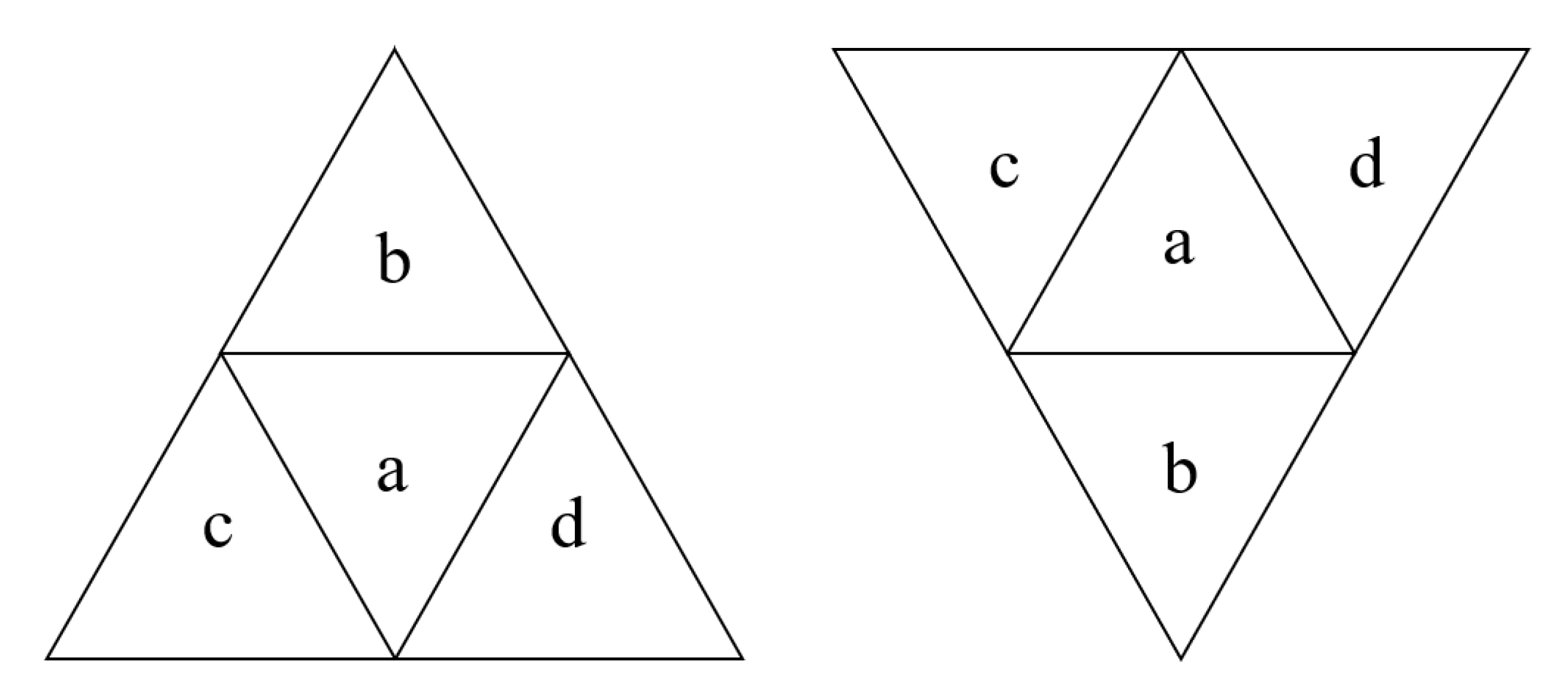
2.2. Encoding Classification

2.2.1. Hierarchical Encoding

The boundaries of the parent and child cells generated by QTM dividing are completely coincident. Their hierarchical relationship is simple and clear, so QTM generally uses hierarchical encoding to establish grid identification.

As shown in Figure 8, “a”, “b”, “c”, and “d” represent the four directions (center, upward (downward), left and right) of the children positioned by the central triangle in the hierarchical division, which are used to represent the directional characteristic of triangle grid encoding. According to the sequence of a-b-c-d, there is 1 case for Goodchild encoding and LS encoding, 2 cases for modified direction encoding, and 4 cases for quaternary coding, as shown in

Table 2. Directivity of QTM encoding.

Encoding Method	a	b	c	d	Arrangement Situation
Goodchild encoding	0	1	2	3	1
LS encoding	10	00	01	11	1
Modified direction encoding	0	1	2	3	2
	0	1	3	2
Quaternary encoding	1	2	0	3	4
	1	2	3	0
	1	0	2	3
	1	0	3	2

. The directionality of the encoding determines the frequency of enumeration judgments in the algorithm design process. The higher the directionality, the more complicated the conversion between the corresponding QTM encoding and the geographic coordinate and the neighbor finding algorithm.

2.2.2. Other Encoding

The encoding methods described above are based on quadtree subdivision of triangular grids. In addition, there are TRQ encoding and arithmetic layer encoding methods. TRQ encoding is based on linear quadtree rhombus grid, which is convenient for data sharing, exchange, and fusion between triangular grid and rhombus grid. Arithmetic layer encoding belongs to integer coordinate coding. Its advantage is to avoid the complex recursive calculation when coding and geospatial coordinate transformation. Its adjacent relationship calculation is simple, however, it loses the hierarchical characteristics of a triangular grid.

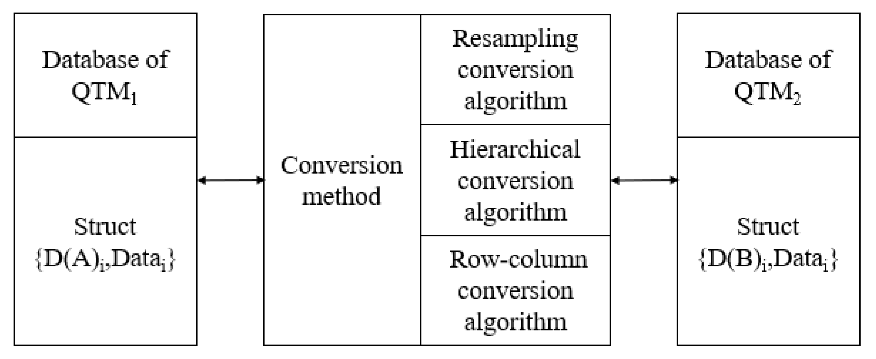
3. Conversion Method

The conversion of QTM encodings provides core algorithms for facilitating data fusion and sharing, and is used for data sharing across QTMs, importing and exporting of QTM databases, etc. Depending on the problem, the encoding of the grid cell is different, but its position and the attribute information contained in it are constant (under the same projection), as shown in Figure 9. The key content of encoding conversion is to establish the mapping rules between different codes, as shown in Figure 10. D(<T>) = {[D(<T>)]_i |i∈N}, where D is the set of encodings, <T> is the category of QTM encodings, and N is the total number of cells in the grid in the study area, such as D(LS) is expressed as a collection of LS encodings.

3.1. Resampling Conversion Algorithm

The resampling conversion method is the calculation process of obtaining the QTM₂ encoding D(B) from the geographic coordinate data set of the grid center points corresponding to the QTM₁ encoding D(A). The specific process is as follows: according to the conversion method of encoding and latitude and longitude, D(A) is converted into the spatial coordinate set$C(x,y,z)=\left\{C{\left(x,y,z\right)}_i|i\in N\right\}$, then D(B) can be calculated from $C\left({x,y,z}_i\right)$, as shown in Figure 11. In the figure, Point₀, Point₁, and Point₂ are the coordinates of the 3 vertices of the grid, and $C\left({x,y,z}_i\right)$ can be obtained according to Equation (1).

$$C({x,y,z}_i)=\frac{Poin{t}_0+Poin{t}_1+Poin{t}_2}{3}$$

(1)

3.2. Hierarchical Conversion Algorithm

The hierarchical conversion method is to replace D(A)_i from front to back step by step to D(B)_i according to the encoding allocation rules in the process of QTM subdivision.

3.2.1. Conversion Rules between Goodchild Encoding and LS Encoding

As mentioned above, the Goodchild encoding and LS encoding have the same characteristics, and the main difference is that the encoding identifiers for the 4 children are different. Therefore, their conversion rules are relatively simple. We only need to swap “0” and “10”, “1” and “00”, “2” and “01”, and “3” and “11” step by step to complete the conversion. According to the correspondence between the two encodings, except for “0” and “1”, the rest are equal after the base conversion. Therefore, in the process of encoding conversion, the “0” and “1” in the fixed direction encoding can be first replaced, and then the obtained quaternary encoding string can be converted into N-bit binary string, which is the LS encoding. Compared with direct conversion, this method reduces the frequency of enumeration in the algorithm, so the time complexity of the algorithm is greatly reduced. The process of extracting Goodchild encoding from LS encoding is the opposite.

3.2.2. Conversion Rules between Goodchild Encoding and Modified Direction Encoding

For the modified direction encoding, the encoding of the left and right children are opposite to those of the Goodchild encoding in the triangular grid with orientation below. According to the subdivision level, the direction of the triangle is judged step by step from the front to the back. If the direction of the triangle is downward, “2” and “3” will be exchanged; otherwise, no changes will be made. The algorithm flow is shown in Figure 12, where GCODE is the Goodchild encoding, and FCODE is the modified direction encoding.

3.2.3. Conversion Rules between Goodchild Encoding and Quaternary Encoding

Although the quaternary coding method ensures the continuity of the index and has the characteristic of a one-dimensional space filling curve, it sacrifices the directionality of the identifier.

Code(Q) represents the quaternary encoding, and Code(Q)[i] is the encoding of the i-th bit of Code(Q)(i < N, where N is the hierarchical level), then Code[i] depends on Code [i-1], and its encoding rules are shown in

Table 3. Quaternary division encoding rule of QTM based on quaternary encoding.

CODE[i]	Direction	CODE[i−1]	a	b	c	d
0	Upward	0, 1, 2	1	2	0	3
		3	1	0	2	3
	Downward	0, 1, 2	1	0	3	2
		3	1	2	3	0
1	Upward	0, 1, 2	1	2	0	3
		3	1	0	2	3
	Downward	0, 1, 2	1	0	3	2
		3	1	2	3	0
2	Upward	0, 1, 2	1	2	0	3
		3	1	0	2	3
	Downward	0, 1, 2	1	0	3	2
		3	1	2	3	0
3	Upward	0, 1, 2	1	0	2	3
		3	1	2	0	3
	Downward	0, 1, 2	1	2	3	0
		3	1	0	3	2

according to triangular grid orientation.

The “a”, “b”, “c”, and “d” in Table 3 can be equivalently replaced by the identifiers “0”, “1”, “2”, and “3” of the four children with Goodchild encodings. Therefore, the conversion between quaternary encoding and Goodchild encoding can be calculated according to the above rules.

3.3. Row–Column Conversion Method

Goodchild encoding, LS encoding, modified direction encoding, and quaternary encoding can complete the encoding conversion step by step through the above algorithms because they belong to the hierarchical encoding of quadtree. The advantage of the hierarchical conversion method is that it avoids a lot of floating number calculation in the resampling conversion method, but it is only limited to the hierarchical encoding of the quadtree division of the triangular grids. However, there are other encoding types of QTM, such as integer coordinate encoding and TRQ encoding. Due to the particularity of the encoding rules, the hierarchical conversion method is not applicable to this type of encoding. In response to this problem, according to the distribution characteristics of the triangular grid, this chapter proposes a row–column conversion method. The row–column encoding set corresponding to the encodings set of QTM is$L(\phi ,\kappa )=\left\{L{(\phi ,\kappa )}_i|i\in N\right\}$. The basic principle of this algorithm is that D(A)_i is converted to row–column number L((φ,κ)i according to the row–column algorithm or the three-orientation translating algorithm, and then L(φ,κ)_i is converted to D(B)_i through the inverse operation, the algorithm flow is shown in Figure 13.

3.3.1. Conversion Algorithm of the QTM Encoding and Row–Column Number

The row–column number of the QTM encoding is the arithmetic layer encoding described in Section 2. As shown in Figure 14, φ is the row number, κ is the column number. For ease of understanding, we convert the triangular grid into a square grid as shown in Figure 15. The following takes Goodchild encoding as an example, we respectively use the row–column algorithm [23] and the three-orientation translating algorithm [24] to calculate the row–column number.

(1) Row and column algorithm

The range of the row number of the triangular grids in a quadrant is φ ∈ [0, 2ⁿ−1] (from the pole to the equator), and the range of the column number is κ ∈ [0, 2φ]. Suppose the encoding of the triangular grid is Code = C₀C₁C₂C₃C₄C₅…C_n−1, where n is the subdivision level. The row–column number is calculated according to the row–column algorithm as described below.

A. Calculation of row number

According to the orientation of the parent triangular grid, set a marker to Q. When Q = 0, its direction is upward, and when Q = 1, its direction is downward. If the direction is different, the row numbers corresponding to the cells are also different, as shown in Figure 14. In the triangular grid of each level, 4 cells can be divided into 2 rows. If the direction of the cell is upward, the row number identifier of the grid encoding as “1” is “0”, and the row number identifier of the grid encoding as “0”, “2”, and “3” is “1”. If the direction of the cell is down, it is completely opposite. The calculation of the row number is as follows: according to Equation (2), a binary string Str = S₀S₁S₂S₃…S_n−1 can be calculated, finally, the row number of the cell can be obtained by converting Str into a decimal number.

$$Str\left[i\right]=\left\{\begin{array}{c}0\left\{\begin{array}{c}Q=0\cup CODE\left[i\right]=1\\ Q=1\cup CODE\left[i\right]=0\cup 2\cup 3\end{array}\right.\\ 1\left\{\begin{array}{c}Q=1\cup CODE\left[i\right]=1\\ Q=0\cup CODE\left[i\right]=0\cup 2\cup 3\end{array}\right.\end{array}\right.$$

(2)

B. Calculation of column number

The κ can be calculated recursively by the φ and the encoding rules. The algorithm is as follows. Among them, the initial value of κ and i are 0, m = φ_max + 1 = 2ⁿ.

①

If CODE[i] = 0, then κ = κ + [2 × (φ − m/2) + 1], φ = m − φ − 1, m = m/2;

②

If CODE[i] = 1, then κ = κ, m = m/2;

③

If CODE[i] = 2, then κ = κ, m = m/2, φ = φ − m;

④

If CODE[i] = 3, then κ = κ + m, m = m/2, φ = φ − m;

⑤

Repeat the above calculations until i = 2ⁿ−1 and output the value of κ.

3) Calculate the encoding from the row–column number

m = φ_max + 1 = 2ⁿ, the algorithm is as follows:

①

If φ < m/2, then CODE[i] = 1, m = m/2, φ = φ − m;

②

If φ ≥ m/2, and κ < (φ+1−m/2), then CODE[i] = 2, m = m/2;

③

If φ ≥ m/2, and κ ≥ m ∩ κ ≥ (φ + 1− m/2), then CODE[i] = 3, κ = κ − 2m;

④

If φ ≥ m/2, and (φ + 1 − m/2) ≤ κ < m, then CODE[i] = 0, κ = κ + m − 2φ −1, m = m/2, φ = φ − m;

⑤

Repeat the above calculations until i = 2ⁿ−1 and output CODE.

(2) Three-orientation translating algorithm

A. Calculation of row–column number

This chapter uses three orientation coordinates to calculate the row–column number of QTM encoding. The three-orientation coordinate system of the triangular grids is shown in Figure 16, where α,β,γ ∈ [0,2ⁿ − 1]. The method of calculating α from the encoding is the same as the row number calculated above, and the calculation of β and γ are similar. Finally, the row number and column number can be calculated according to Equation (3).

$$\left\{\begin{array}{c}\phi =\alpha \\ =\alpha +\gamma -\beta \end{array}\right.$$

(3)

B. Calculate the encoding from the row–column number

According to the properties of the three-orientation coordinate system, it can be obtained as follows: if the direction of the grid is upward, then α + β + γ = 2ⁿ, otherwise α + β + γ = 2ⁿ + 1. Therefore, the direction of the triangular grid can be determined according to the sum of α, β, and γ. At the same time, because of the row–column coordinates of the triangular grid, when k is an odd number, the direction of the grid is downward, and when k is non-odd, the direction of the grid is upward. Combining the two properties can result in another relationship between the row–column number and the three-orientation coordinate, such as Equation (4) and Equation (5). Combining the two formulas can calculate the three-orientation coordinates of the grid cell from the row–column number.

$$\left\{\begin{array}{c}\phi =\alpha \\ \gamma -\beta =-\alpha \end{array}\right.$$

(4)

$$\left\{\begin{array}{c}\alpha +\beta +\gamma =2^n, k\%2=0\\ \alpha +\beta +\gamma =2^n+1, k\%2=1\end{array}\right.$$

(5)

After obtaining the three-orientation coordinates of the grid, the algorithm flow of calculating the encoding according to the three-orientation coordinates is as follows:

①

Convert α, β, γ into n-bit binary strings Str_α, Str_β, Str_γ, where n is the subdivision level;

②

According to the rules in

Table 4. Correspondence rules of three-orientation coordinates and encodings.

Identifiers at Each Level	Encoding of Triangles
	Upward Triangle	Downward Triangle
Strα[i] = 0	1	0, 2, 3
Strα[i] = 1	0, 2, 3	1
Strβ[i] = 0	3	0, 1, 2
Strβ[i] = 1	0, 1, 2	3
Strγ[i] = 0	2	0, 1, 3
Strγ[i] = 1	0, 1, 3	2

, the encoding are calculated from Strα[i], Strβ[i], and Str_γ[i], and the same value in the encodings corresponding to the three level identifiers is the desired encoding;

③

Repeat the above steps until the calculation is completed.

(3) Algorithm efficiency analysis

We used all the triangular grids within a hexagram limit (subdivision level 6–12) as the experimental objects and calculated the time consumption with the above two algorithms, respectively, and finally compared and analyzed the experimental results, as shown in

Table 5. Algorithmic efficiency of encoding conversion to row–column number.

Subdivision Level	The Number of Cells in the Grid	Time (s)		Average Number of Conversions of 1s		Algorithm (1) 1 Time/Algorithm (2) 2 Time
		Algorithm (1) 1	Algorithm (2) 2	Algorithm (1) 1	Algorithm (2) 2
6	4096	0.013	0.008	315,077	512,000	62%
7	16,384	0.057	0.035	287,439	468,114	61%
8	65,536	0.246	0.149	266,407	439,839	61%
9	262,144	1.050	0.643	249,661	407,689	61%
10	1,048,576	4.506	2.715	232,707	386,216	60%
11	4,194,304	17.789	10.695	235,781	392,174	60%
12	16,777,216	72.894	43.565	230,159	385,108	60%

¹ Row–column algorithm. ² Three-orientation translating algorithm.

and

Table 6. Algorithmic efficiency of row–column number conversion to encoding.

Subdivision Level	The Number of Cells in the Grid	Time (s)		Average Number of Conversions of 1s		Algorithm (1) 1 Time/Algorithm (2) 2 Time
		Algorithm (1) 1	Algorithm 2) 2	Algorithm (1) 1	Algorithm (2) 2
6	4096	0.006	0.014	682,667	292,571	43
7	16,384	0.025	0.058	655,360	282,483	43
8	65,536	0.103	0.243	638,504	269,695	42
9	262,144	0.436	1.048	601,248	250,137	42
10	1,048,576	1.844	4.534	568,642	231,270	41
11	4,194,304	7.568	18.459	554,216	227,223	41
12	16,777,216	30.589	74.973	548,472	223,777	41

¹ Row–column algorithm. ² Three-orientation translating algorithm.

. Among them, the computer hardware environment is DELL T3620, 8-core Intel(R) Core (TM) i7-7700 CPU @ 3.60 GHZ processor, RAM 32.0 Gb, and Win10 Professional Edition.

Through analysis, we can get the following conclusions:

A. In the conversion algorithm from encoding to row–column number, the row number calculation in the row–column algorithm is consistent with the calculation logic of α, β, and γ in the three-orientation coordinate positioning algorithm, and the algorithm execution process is simple because their time consumption is mainly concentrated in the process of calculating the binary identifier from the quaternary encoding. However, the calculation of the column number in the row–column algorithm is more complicated. In the step by step recursive process of the algorithm, there are many parameters that need to be calculated and changed. Therefore, the three-orientation coordinate positioning algorithm is more efficient. As shown in Figure 17, Figure 18, and Table 4, the three-orientation coordinate positioning algorithm is 1.67 times that of the row–column algorithm.

B. In the conversion algorithm from the row–column number to encoding, the logic of the three-orientation coordinate positioning algorithm is simple; however, the process of calculating the encoding from the binary string is relatively cumbersome. On the contrary, although the logic of the row–column algorithm is complicated, the computational workload is relatively small. As shown in Figure 18 and Table 5, the row–column algorithm is 2.5 times that of the three-orientation coordinate positioning algorithm.

In summary, we will use the three-orientation coordinate positioning algorithm and the row–column algorithm to process the conversion of encoding to row-column number and the conversion of row–column number to encoding respectively.

3.3.2. Conversion Algorithm of the TRQ Encoding and Row–Column Number

The rhombus grid based on linear quadtree has a natural Morton encoding coordinate system [25], as shown in Figure 19, where I and J indicate the position of a rhombus grid. Morton encoding (M_code = M₀M₁M₂M₃…M_n−1) can be represented by Mcode = 2I + J.

(1) Calculation of row–column number

The encoding of triangular grids based on linear quadtree rhombic grids division can be suffixed “0” and “1”in M_code to distinguish upward and downward triangles. According to Equation (6), the transformation between the IJ and φκ coordinate system (as shown in Figure 20) can be realized by using spatial similarity transformation. Finally, according to the correspondence between the triangular grid and the rhombus grid (as shown in Figure 21) and the orientation of the triangular grid, the row–column number of the triangular grid can be calculated by Equation (7).

$$\left[\begin{array}{c}{\phi }_D\\ {\kappa }_D\end{array}\right]=\left[\begin{array}{cc}-1& 1\\ 0& 1\end{array}\right]\left[\begin{array}{c}I\\ J\end{array}\right]+\left[\begin{array}{c}{2}^n-1\\ 0\end{array}\right]$$

(6)

$$\left\{\begin{array}{c}{\phi }_T=\left\{\begin{array}{c}{\phi }_D,Q=0\\ {\phi }_D+1,Q=1\end{array}\right.\\ {\kappa }_T=\left\{\begin{array}{c}{\mathrm{2\kappa }}_D,Q=0\\ {\mathrm{2\kappa }}_D-1,Q=1\end{array}\right.\end{array}\right.$$

(7)

where, (φ_T, κ_T) and (φ_D, κ_D) are the row–column numbers of the diamond and triangle grids in the φκ coordinate system, respectively; (I, J) is the row–column coordinates of the diamond grid in the IJ coordinate system; if Q = 0, the direction of the triangle is upward, and Q = 1 is the opposite; $\left[\begin{array}{cc}-1& 1\\ 0& 1\end{array}\right]$ is the rotation matrix between different coordinate systems; and $\left[\begin{array}{c}{2}^{n-1}\\ 0\end{array}\right]$ is the coordinate of the origin of the φκ coordinate system in the IJ coordinate system.

(2) Calculate the encoding from the row–column number.

①

First the rhombic grid coordinates φ_D, κ_D; in the φκ coordinate system can be obtained by inverse calculation using Equation (8) and the row–column number of the triangular grid;

②

Then it uses the Equation (9) and φ_D, κ_D to obtain the coordinates of the rhombic grid in the IJ coordinate system, and converts I and J to the diamond grid encoding;

③

Finally, according to the orientation of the triangle and the encoding rules, the TRQ encoding of the triangular grid can be obtained.

$$\left\{\begin{array}{c}{\phi }_D=\left\{\begin{array}{c}{\phi }_T,{\kappa }_T\%2=0\\ {\phi }_T-1,{\kappa }_T\%2=1\end{array}\right.\\ {\kappa }_D=\left\{\begin{array}{c}\frac{{\kappa }_T}{2},{\kappa }_T\%2=0\\ \frac{{\kappa }_T+1}{2},{\kappa }_T\%2=0\end{array}\right.\end{array}\right.$$

(8)

$$\left[\begin{array}{c}I\\ \mathrm{J}\end{array}\right]=\left[\begin{array}{cc}-1& 1\\ 0& 1\end{array}\right]\left[\begin{array}{c}{\phi }_D\\ {\kappa }_D\end{array}\right]+\left[\begin{array}{c}{2}^n-1\\ 0\end{array}\right]$$

(9)

4. Comparison and Analysis of Algorithm Efficiency

We used the 2015 average annual rainfall grid data of Inner Mongolia from the 9th to 13th levels as the experimental object (data from the Institute of Geographic Sciences and Natural Resources Research, Chinese Academy of Sciences http://www.resdc.cn/, accessed on 20 December 2021), as shown in Figure 22, and calculated the time consumption with the above three algorithms, respectively. Among them, the QTM construction method is great arc division [15], and the hardware environment is the same as described above.

4.1. Comparative Analysis of Conversion Algorithms of Hierarchical Encoding

(1) Comparative analysis of resampling algorithm and hierarchical conversion algorithm

Both of these algorithms use recursive methods, and their time complexity is O(4ⁿ). In terms of a single operation, the resampling conversion algorithm is mainly based on the conversion between encoding and space coordinates, involving floating-point number multiplication, square root and other operations, and the calculation is complex. The hierarchical conversion algorithm is the integer conversion of the quaternary system, or the conversion between quaternary system and binary system, and the calculation is relatively simple. However, the resampling conversion algorithm has a wide range of applications, and can be used for any conversion of projection, subdivision, and coding. The level conversion algorithm is limited to the conversion of the same projection and subdivision. The experimental results are shown in

Table 7. Comparison table of the algorithms efficiency of conversion from Goodchild encoding to LS encoding.

Subdivision Level	The Number of Cells in the Grid	Time (s)		Average Number of Conversions of 1s		Algorithm (1) 1 time/Algorithm (2) 2 Time
		Algorithm (1) 1	Algorithm (2) 2	Algorithm (1) 1	Algorithm (2) 2
9	3455	0.019	0.004	181,842	909,211	20%
10	14,653	0.084	0.017	174,440	861,941	20%
11	57,087	0.357	0.072	159,908	792,875	20%
12	225,264	1.445	0.290	155,892	776,772	20%
13	894,665	5.849	1.171	152,960	764,018	20%
14	3,587,606	23.688	4.766	151,452	752,750	20%
15	14,386,302	96.056	19.334	149,770	744,093	20%

¹ Resampling conversion algorithm. ² Hierarchical conversion algorithm.

,

Table 8. Comparison table of the algorithms efficiency of conversion from Goodchild encoding to modified direction encoding.

Subdivision Level	The Number of Cells in the Grid	Time (s)		Average Number of Conversions of 1s		Algorithm (1) 1 Time/Algorithm (2) 2 Time
		Algorithm (1) 1	Algorithm (2) 2	Algorithm (1) 1	Algorithm (2) 2
9	3455	0.016	0.008	215,938	431,875	50%
10	14,653	0.07	0.035	209,329	418,657	50%
11	57,087	0.283	0.142	201,721	402,021	50%
12	225,264	1.177	0.579	191,388	389,057	49%
13	894,665	4.944	2.398	180,960	373,088	49%
14	3,587,606	20.918	10.25	171,508	350,010	49%
15	14,386,302	88.692	43.637	162,205	329,681	49%

¹ Resampling conversion algorithm. ² Hierarchical conversion algorithm.

and

Table 9. Comparison table of the algorithms efficiency of conversion from Goodchild encoding to quaternary encoding.

Subdivision Level	The Number of Cells in the Grid	Time (s)		Average Number of Conversions of 1s		Algorithm (1) 1 Time/Algorithm (2) 2 Time
		Algorithm (1) 1	Algorithm (2) 2	Algorithm (1) 1	Algorithm (2) 2
9	3455	0.021	0.013	164,524	265,769	62%
10	14,653	0.092	0.056	159,272	261,661	61%
11	57,087	0.399	0.239	143,075	238,858	60%
12	225,264	1.632	0.958	138,029	235,140	59%
13	894,665	6.669	3.883	134,153	230,406	58%
14	3,587,606	27.276	15.820	131,530	226,777	58%
15	14,386,302	112.104	64.796	128,330	222,025	58%

¹ Resampling conversion algorithm. ² Hierarchical conversion algorithm.

and Figure 23. The analysis shows that for the conversion between different encodings, the conversion efficiency of the hierarchical conversion algorithm is better than that of the resampling algorithm.

(2) Analysis of the relationship between directivity and encoding conversion efficiency

The following conclusions can be obtained by comparison of the relationship between the encoded directivity conversion efficiency. The complexity of the encoding conversion mapping rule depends on the complexity of the encoding directionality, and the direction complexity is inversely proportional to the encoding conversion efficiency, as shown in Figure 24.

4.2. Comparison and Analysis of Conversion Algorithm Efficiency of Other Types of Encoding

For TRQ encoding, it does not have the hierarchical characteristics of triangles, so it is necessary to use the “row–column number" as an intermediary for encoding conversion. Therefore, the row–column conversion algorithm is similar to the resampling algorithm, and they both need a medium as a bridge for conversion. However, like the hierarchical conversion algorithm, the row–column conversion algorithm avoids the calculation of floating-point numbers. The analysis of the experimental results is shown in

Table 10. Comparison table of the algorithms efficiency of conversion from Goodchild encoding to TRQ encoding.

Subdivision Level	Number of Grids	Time (s)		Average Number of Conversions of 1s		Algorithm (1) 1/Algorithm(2) 2
		Algorithm (1) 1	Algorithm (2) 2	Algorithm (1) 1	Algorithm (2) 2
9	3455	0.016	0.014	215,938	246,786	88
10	14,653	0.072	0.063	203,514	232,587	88
11	57,087	0.306	0.268	186,559	213,011	88
12	225,264	1.243	1.080	181,226	208,578	87
13	894,665	5.116	4.476	174,876	199,880	87
14	3,587,606	21.054	18.103	170,400	198,177	86
15	14,386,302	87.051	74.863	165,263	192,168	86

¹ Resampling conversion algorithm. ² Row–column conversion algorithm.

and

Table 11. Comparison table of the algorithms efficiency of conversion from TRQ encoding to Goodchild encoding.

Subdivision Level	Number of Grids	Time (s)		Average Number of Conversions of 1s		Algorithm (1) 1/Algorithm(2) 2
		Algorithm (1) 1	Algorithm (2) 2	Algorithm (1) 1	Algorithm (2) 2
9	3455	0.018	0.012	191,944	287,917	67
10	14,653	0.079	0.052	185,481	280,709	66
11	57,087	0.341	0.225	167,411	253,720	66
12	225,264	1.395	0.919	161,480	245,119	66
13	894,665	5.638	3.703	158,685	241,605	66
14	3,587,606	23.061	14.992	155,570	239,301	65
15	14,386,302	93.355	60.680	154,103	237,085	65

¹ Resampling conversion algorithm. ² Row–column conversion algorithm.

and Figure 25 and Figure 26. Compared with the resampling conversion algorithm, the row–column conversion algorithm is more efficient, and the difference between the conversion efficiency of Goodchild encoding and TRQ encoding is mainly reflected in the complexity of the encoding and row–column number conversion algorithm.

5. Conclusions

This paper proposes three conversion algorithms for QTM encoding. The main research results are as follows: Firstly, based on the research of QTM encoding characteristics classification, we put forward a directional feature to measure the complexity of encoding conversion, and there is a negative correlation between directional complexity and encoding conversion efficiency. Then, this paper proposes the resampling conversion algorithm, hierarchical conversion algorithm, and row–column conversion algorithm of QTM encoding according to the relationship between the encoding and spatial coordinates, the directionality of the encoding, and the row–column encoding of the grid. In addition, through experimental verification, it can be seen that the efficiency of the hierarchical conversion algorithm and the rank conversion algorithm is higher. Finally, this paper proposes an algorithm for interchange of TRQ encoding and row–column number, and compares the two methods of conversion between QTM encoding and row–column number. The results show that when the row number and column number are calculated by QTM, the three-axis coordinate positioning algorithm is better, otherwise the row-column algorithm is better. In summary, the encoding conversion algorithm proposed in this article provides a theoretical and technical basis for the interoperability of QTM encoding. At the same time, the above row–column conversion algorithm can also be applied to the conversion between QTM and rhombus grids.

References

1. Purss, M.B.; Peterson, P.R.; Strobl, P.; Dow, C.; Sabeur, Z.A.; Gibb, R.G.; Ben, J. Datacubes: A discrete global grid systems perspective. Cartogr. Int. J. Geogr. Inf. Geovis. 2019, 54, 63–71. [Google Scholar] [CrossRef]
2. Yao, X.; Li, G.; Xia, J.; Ben, J.; Cao, Q.; Zhao, L.; Ma, Y.; Zhang, L.; Zhu, D. Enabling the big earth observation data via cloud computing and DGGS: Opportunities and challenges. Remote Sens. 2019, 12, 62. [Google Scholar] [CrossRef] [Green Version]
3. Kolar, J. Representation of the geographic terrain surface using global indexing. In Proceedings of the 12th International Conference on Geoinformatics, Gävle, Sweden, 7–9 June 2004; pp. 321–328. [Google Scholar]
4. Zhao, X.S.; Ben, J.; Sun, W.B.; Tong, X. Overview of the research progress in the earth tessellation grid. Acta Geod. Et Cartogr. Sin. 2016, 45, 1–14. [Google Scholar]
5. Dutton, G.H. A Hierarchical Coordinate System for Geoprocessing and Cartography; Spring: Berlin/Heidelberg, Germany, 1999; p. 23. [Google Scholar]
6. Goodchild, M.F. Reimagining the history of GIS. Ann. GIS 2018, 24, 1–8. [Google Scholar] [CrossRef]
7. Dutton, G. Modeling Locational Uncertainty via Hierarchical Tesselation: Accuracy of Spatial Database; Taylor and Francis: London, UK, 1989; pp. 125–140. [Google Scholar]
8. Hou, M.; Xing, H.; Zhao, X.; Chen, J. Computing of complicated topological relation in spherical surface quaternary triangular mesh. Geomat. Inf. Sci. Wuhan Univ. 2012, 37, 468–470. [Google Scholar]
9. Fekete, G. Rendering and managing spherical data with sphere quadtrees. In Proceedings of the First 1990 IEEE Conference on Visualization, San Francisco, CA, USA, 23–26 October 1990; pp. 176–186. [Google Scholar]
10. Goodchild, M.F.; Yang, S. A hierarchical spatial data structure for global geographic information systems. CVGIP Graph. Models Image Processing 1992, 54, 31–44. [Google Scholar] [CrossRef] [Green Version]
11. Dutton, G. Digital map generalization using a hierarchical coordinate system. In Proceedings of the Auto Carto 13, Bethesda, MD, USA, 7–10 April 1997; ACSM/AS-PRS. pp. 367–376. [Google Scholar]
12. Dutton, G. Scale, sinuosity and point selection in digital line generalization. Cartogr. Geogr. Inf. Sci. 1999, 26, 33–53. [Google Scholar] [CrossRef]
13. Lee, M.; Samet, H. Navigating through triangle meshes implemented as linear quadtree. ACM Trans. Graph. 2000, 19, 79–121. [Google Scholar] [CrossRef]
14. Chen, Y.H.; Wang, J.X.; Cao, Z.N. The uniform encoding and generation method of structure elements of Discrete Global Grid Systems. J. Geo-Inf. Sci. 2021, 23, 1382–1390. [Google Scholar]
15. Amiri, A.M.; Samavati, F.; Peterson, P. Categorization and conversions for indexing methods of discrete global grid systems. Int. J. Geo-Inf. 2015, 4, 320–336. [Google Scholar] [CrossRef]
16. Du, L.Y.; Ben, J.; Maq, H. An algorithm for generating discrete line transformation of planar triangular grid based on weak duality. Geomat. Inf. Sci. Wuhan Univ. 2020, 45, 105–110. [Google Scholar]
17. Amiri, A.M.; Harrison, E.; Samavati, F. Hexagonal connectivity maps for Digital Earth. Int. J. Digit. Earth 2015, 8, 750–769. [Google Scholar] [CrossRef]
18. Ben, J.; Tong, X.C.; Zhou, C.H.; Zhang, K.X. Construction algorithm of octahedron based hexagon grid systems. J. Geo-Inf. Sci. 2015, 17, 789–797. [Google Scholar]
19. Gold, C.; Mostafavi, M.A. Towards the global GIS. ISPRS J. Photogramm. Remote Sens. 2000, 55, 150–163. [Google Scholar] [CrossRef]
20. Bartholdi, J.J.; Goldsman, P. Continuous indexing of hierarchical subdivisions of the globe. Int. J. Geogr. Inf. Sci. 2001, 15, 489–522. [Google Scholar] [CrossRef] [Green Version]
21. Wang, J.X.; Chen, Y.H.; Cao, Z.N.; Qin, Z.; Shi, Y. Algorithm of neighbor finding on quaternary triangular mesh with modified direction coding. Sci. Surv. Mapp. 2021, 46, 196–202. [Google Scholar]
22. Bai, J.J.; Zhao, X.S.; Chen, J. Indexing of discrete global grids using linear quadtree. Geomat. Inf. Sci. Wuhan Univ. 2005, 30, 805–808. [Google Scholar]
23. Zhao, X.S.; Chen, J. Fast translating algorithm between QTM code and longitude/latitude coordination. Acta Geod. Cartogr. Sin. 2003, 32, 272–277. [Google Scholar]
24. Tong, X.C.; Zhang, Y.S.; Ben, J. Three orientation translating algorithm of long./lat. coordination and QTM code along with its criterion judge of precision. Geomat. Inf. Sci. Wuhan Univ. 2006, 31, 27–30. [Google Scholar]
25. White, D. Global grids from recursive diamond subdivisions of the surface of an octahedron or icosahedron. Environ. Monit. Assess. 2000, 64, 93–103. [Google Scholar] [CrossRef]
Figure 1. Schematic diagram of level 3 QTM.
Ijgi 11 00033 g001
Figure 2. Goodchild encoding method.
Ijgi 11 00033 g002
Figure 3. Goodchild encoding method.
Ijgi 11 00033 g003
Figure 4. Modified direction encoding method.
Ijgi 11 00033 g004
Figure 5. Quaternary encoding method.
Ijgi 11 00033 g005
Figure 6. TRQ encoding method.
Ijgi 11 00033 g006
Figure 7. Arithmetic layer encoding method.
Ijgi 11 00033 g007
Figure 8. The direction encoding.
Ijgi 11 00033 g008
Figure 9. Encoding conversion diagram of QTM1 and QTM2.
Ijgi 11 00033 g009
Figure 10. Conceptual diagram of QTM encoding conversion.
Ijgi 11 00033 g010
Figure 11. Flow chart of resampling conversion method.
Ijgi 11 00033 g011
Figure 12. Algorithm flow chart of conversion from Goodchild encoding to modified direction encoding.
Ijgi 11 00033 g012
Figure 13. Algorithm flow chart of QTM encoding through the row–column conversion method.
Ijgi 11 00033 g013
Figure 14. Schematic diagram of row–column encoding.
Ijgi 11 00033 g014
Figure 15. Schematic diagram of simplified row–column encoding.
Ijgi 11 00033 g015
Figure 16. The three-orientation coordinate system of the triangular grids.
Ijgi 11 00033 g016
Figure 17. The algorithm efficiency analysis diagram of encoding conversion to row–column number.
Ijgi 11 00033 g017
Figure 18. The algorithm efficiency analysis diagram of row–column number conversion to encoding.
Ijgi 11 00033 g018
Figure 19. Linear quadtree encoding based on Morton encoding coordinate System.
Ijgi 11 00033 g019
Figure 20. The φκ coordinate system of the rhombic grid.
Ijgi 11 00033 g020
Figure 21. The φκ coordinate system of triangular grids based on linear quadtree rhombic discrete grids.
Ijgi 11 00033 g021
Figure 22. Inner Mongolia’s average annual rainfall in 2015.
Ijgi 11 00033 g022
Figure 23. Comparison of efficiency between resampling algorithm and hierarchical conversion algorithm.
Ijgi 11 00033 g023
Figure 24. Efficiency of hierarchical conversion algorithms for different types of encoding.
Ijgi 11 00033 g024
Figure 25. The time-consumption of the algorithms of conversion from Goodchild encoding to TRQ encoding.
Ijgi 11 00033 g025
Figure 26. The time-consumption of the algorithms of conversion from TRQ encoding to Goodchild encoding.
Ijgi 11 00033 g026