Evaluation of Community Livability Using Gridded Basic Urban Geographical Data—A Case Study of Wuhan

Abstract

The evaluation of community livability quantifies the demands of human settlement at the micro scale, supporting urban governance decision-making at the macro scale. Big data generated by the urban management of government agencies can provide an accurate, real-time, and rich data set for livability evaluation. However, these data are intertwined by overlapping geographical management boundaries of different government agencies. It causes the difficulty of data integration and utilization when evaluating community livability. To address this problem, this paper proposes a scheme of partitioning basic geographical space into grids by optimally integrating various geographical management boundaries relevant to enterprise-level big data. Furthermore, the system of indexes on community livability is created, and the evaluation model of community livability is constructed. Taking Wuhan as an example, the effectiveness of the model is verified. After the evaluation, the experimental results show that the livability evaluation with reference to our basic geographic grids can effectively make use of governmental big data to spatially identify the multi-dimensional characteristics of a community, including management, environment, facility services, safety, and health. Our technical solution to evaluate community livability using gridded basic urban geographical data is of large potential in producing thematic data of community, constructing a 15-min community living circle of Wuhan, and enhancing the ability of the community to resist risks.

1. Introduction

Building safe and livable cities has become a global focus. Large-scale, large-population, and complex environments associated with the progression of urbanization and globalization have created great challenges to urban construction and development [1]. For instance, the difficulties in the abatement and mitigation of the Coronavirus epidemic in 2020 have revealed the shortage of public resources and services, and further delayed the responses to public emergencies. The goal of livable human settlements is to build inclusive, safe, resilient, and sustainable communities [2]. Based on the goal and principles of livability, we argue that evaluating the livability of a community is beneficial to citizen-oriented community governance.

In the existing research, urban livability is divided into three levels [3] (

Table 1. Evaluation livability of three levels.

Research Level	Evaluation Object	Evaluation Content
Macro level	Metropolis, city or urban area	Urban economy, culture, environment, education, and medical care of city.
Meso level	Administrative district, urban functional area or rural area	Regional geography, urban function, economic status, transportation, and public facility resources
Micro level	Community, residential quarter	Community management and service, community facility provision, public security, sense of community

). At the macro level, urban livability measures the pressure on citizen living space and the environmental burden of industrialization [4], focusing on an evaluation system constructed by the urban economy, culture, environment, education, and medical care of the whole city [5,6]. At the meso level, livability is analyzed at a set of administrative boundaries of government agencies and urban functional areas [7], whose working content and indicators are domain-specific. The administrative district or street sector has insight into urban space with an emphasis on heterogeneity in regional geography, urban function, economic status, transportation, and public facility resources. At the micro level, there are the community or residential quarters. At these smaller scales, the study of livability is related to the population, income, culture, architectural style, and other attributes of the community [8]. The sustainable development community is a representative livable community in the United States, and it proposes environmental, population, youth education, and health indicators [9]. Mohammadamin Khorasani considers that livable communities should have affordable housing choices, and safe and convenient, walkable transportation conditions [10]. Wei discusses the livability of subsidized housing estates in the residential policy field [11]. Community management and service, community facility provision, public security, sense of community have been discussed in literature to construct a multi-perspective, multi-level research framework [9,10,11]. However, there are some limitations. The indicators of community livability are constructed according to specific conditions [3,11]. It rarely considers the features, public security, management efficiency, and the matching of public facilities and population of the community inner. It is difficult to compare horizontally in a certain period of time and in a certain area [12], especially to identify spatial heterogeneity in facilities, services, safety in the inner city. As the basic unit of community governance, the livability of community-based units is an ideal method to reflect and collect issues of local concern [13]. We argue that the goal of livability evaluation helps to build livable, employable, and travelable communities. Hence, it is necessary to use government data to evaluate community livability from the perspective of the community unit. It can not only precisely describe the urban livability, shorten the period of evaluation, but also identify the coordination between people and the environment as it pertains to the life quality of residents and the healthy development of the city.

For the sake of community livability evaluation, we need to establish a flexible evaluation model [14,15,16] based on the multi-dimensional factors, such as community development, economic status, physical environment, and resident demands. Traditional methodologies are used to evaluate urban livability, such as qualitative Delphi methods, an analytical hierarchy process (such as the technique for order preference by similarity for ideal solution (TOPSIS) and entropy), cluster analysis, factor analysis, principle component analysis, geographic information system (GIS) and spatial modeling, Economist Intelligence Unit and Mercer city rankings, comprehensive marking or standard method, the livable level integrated index, neural networks and global livable cities index (GLC) [17]. AHP is suitable to transform quantitative and qualitative criteria into numerical scales, which have been extensively utilized in a wide variety of areas [18]. The reliability of results in the AHP method depends on the objectivity of the parameters and weights. In order to make the evaluation more convincing, some studies tried to extract livability-related index data from high-resolution remote sensing images and Internet big data [18]. It is known that the accuracy of the data source and data extraction affects the reliability of livability evaluation results [18,19]. A more reliable data source is mainly the micro data from the government information system, stored in different thematic and spatial units. For example, data concerning population, houses, urban facilities, and the economy status of the community are distributed across the sectors of urban household, urban management, fire control, and social governance grids. There are few studies on the integration of multi-source government data to evaluate the livability of communities. Critically, the inconsistent boundaries of these spatial management sectors may lead to data redundancy and conflicts, which statistically causes a spurious correlation. Thus, the accuracy of data analysis cannot meet the demand of livability evaluation. Likewise, the modifiable areal unit problem exists in multi-level livability evaluation. Geographical grid size and geographical grid shape resulting from space partition will affect the accuracy of a livability evaluation [20]. Therefore, this paper discusses how to integrate these geographic grids of multi-source spatial data to reveal the differences in resource allocation and quality difference among communities, which is of great scientific and practical significance in promoting a high-quality development of communities.

The critical issues in community livability evaluation are addressed here. They are the geographical mismatch between administrative boundaries used for data collection by governmental agencies and the integration of these diverse data into a single comprehensive weight of livability. This study proposes a scheme of extracting the basic geographical grids with the relatively permanent and clear boundary of each geographical object. Furthermore, the community livability evaluation model is constructed. Particularly, this study pays more attention to the spatial characteristics of community livability and demonstrates the rationality of the community livability evaluation model. This study is aimed at: (1) generating basic geographical grids concerning the multiple demands of community governance, while integrating human settlement data with irregular grids; (2) constructing an evaluation model of community livability for identifying the fine-grained community public services, human settlements, and public security, for rationalizing public resources allocation, social governance modernization, and sustainable development.

2. Materials and Methods

2.1. Study Area

The study area is in central Wuhan, the capital city of Hubei province, China. The long-term development plan of Wuhan in 2049 envisions the city as an international metropolis that is green, livable, efficient, and energetic [21]. Figure 1 shows the study area of Wuhan, containing six administrative districts and 916 communities, approximately the total area of 545.57 km², and the population of 5,339,728 people [22]. The government has built many information systems to improve city management, such as the information infrastructure, environmental information system, urban management information system. In these systems, the conflicts between management boundaries stemming from fuzzy responsibilities and standards of urban management mainly induces difficulty in data application in central city. Therefore, a central urban area was selected to test our proposed approach for integrative analysis of big data with reference to various geographical grids.

In Figure 1a, the dark part represents the central urban area in relation to the rivers that connect and divide the city, and the administrative districts are explicit. The grey part in Figure 1b shows all the bounded communities located in the central urban area. In this area, data used to evaluate community livability comes from different information systems owned by different government agencies, who are in charge of their own administrative regions. Therefore, data normalization needs to be done before multi-source urban data analysis and community livability evaluation.

2.2. Data and Data Processing

This section introduces the proposed approach to partitioning geographical space into basic grids and integrating data of livability evaluation. These data are big data stored in several government information systems and are spatially referenced with domain-specific grids (Figure 2).

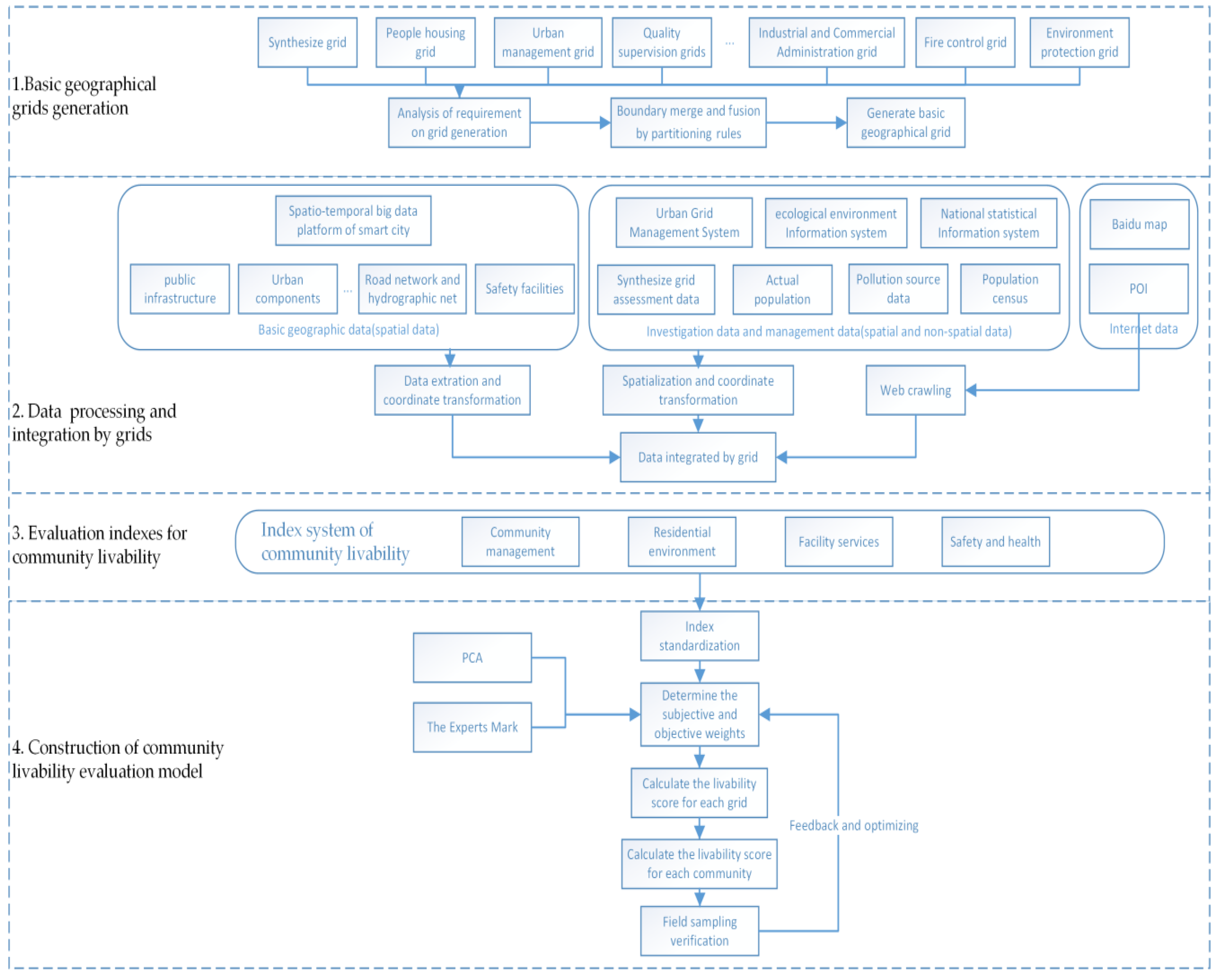
Figure 2 shows the entire technical process of grid-based livability evaluation. From top to bottom, it is divided into four stages: basic geographical grid generation, data processing and spatial data integration, the evaluation indicators establishment, and the construction of a livability evaluation model. In the first stage, generalized rules were established based on the requirements of multi-specialized grids, and then basic geographical grids were generated. In the second stage, major data from spatial and non-spatial datasets of the government information systems were collected, and subsidiary crowd-sourced data were downloaded in a timely manner through the Internet. These data were transformed to unify coordinate system, matched with the address database to link to a latest unique spatial grid by spatial location. In this way, it overcomes the incompatibility in various spatial management grids from different government agencies. A system of index on community livability was established in the third stage. In the last stage, critically, the data were quantified and standarlized, the livability was scored using principal component analysis that combined subjective and objective weights. The reliability of the results was verified by field surveying. The technical details are discussed in the following subsections.

2.2.1. Basic Geographical Grids Generated by Integrating Domain-Specific Grids

Requirements on Grid Generation

We define a basic grid set as a partition of geographical space based on the overlapping boundaries from government agencies that some may traverse a community. Mathematically, the grid system is one partition of continuous space, for integration, organization, management, and sharing of spatial information resources [23]. Such a grid system will serve the compatibility and information exchange of gridded data from various urban management sectors in charge of water, fire, zoning, and social data management. In urban management, these geographic grids refer to diverse physical and social data in real-time from government information systems. Figure 3 shows four kinds of domain-specific grid boundaries.

The size of the grid in Figure 3a–d increases successively, and originally the boundaries of the grid are inconsistent and crossed. It indicates that there are differences in geographical boundaries assigned by the responsibilities of various governmental sectors, and actually none of the grid systems are used in urban management, industry and commerce, environmental protection, food, and medical quality supervision. In Figure 3a,b, the management grid is mostly within 100 hectares, which indicates that urban components, events, and enterprise data generated by urban management, industrial and commercial supervision are concentrated in small grids. In addition, the study area without covering the grids means the non-clear or empty of the corresponding regional responsibility assignment and the lack of data. In Figure 3c,d the management grid is at street scale, and the corresponding data density of environment monitoring, food, and medical law enforcement events is relatively low. Figure 3e shows the overlap and the conflicts in space by professional grids. As a result, the basic data in different management grids cannot be related and shared due to the relatively independent semantics of various grids with different sizes and spatial shapes. Therefore, it is necessary for us to generate a set of basic grids by comprehensively considering issues of management objects, data availability, application decisions, and time-varying characteristics.

Partitioning Rules

The purpose of grid partition is to construct a set of spatial basic cells resolving the conflicts of multi-level management boundaries. Both the spatial relationship of management boundaries existing and the basic data integration of different management boundaries should be modeled in this set of spatial basic cells. The rational grid partition should be compatible with management boundaries as far as possible when dealing with various contradictions of urban management boundaries, so that the spatial basic cell is stable and easy to combine into large-scale management units. The partition result should be of most irregularity, technical expansibility, and universality in urban agency. Specifically, it should obey the following criteria:

(1)

Accuracy of spatial data. The spatial partitioning of geographical grids needs to be in the same coordinate system with urban basic geographical information, so as to keep the consistency of spatial reference.

(2)

Boundary stability. The partition of the basic geographic grid should cover the whole space without gaps or overlaps and minimize the changes in the original grid boundary as much as possible. In this way, the grid is relatively stable and easy to maintain.

(3)

Identification and classification. The residential content inside the grid should be homogenous. The land use type inside the grid shall be the same one as far as possible, with significant characteristics.

(4)

Geographical integrity. The grid boundary must not split geographical features and urban facilities like water resources, transportations, and buildings.

(5)

Balancing management capacities. Multiple factors need to be coordinated in each grid. The public infrastructure allocation and urban management capacity in each grid should be balanced.

In terms of these criteria, the partition grid can mostly undertake the tasks of association, expression, extraction, and combination of different management data consistently gridded with a reference system.

Basic Grid Generation

A basic grid system is the result of geospatial partition and coordination for the sake of integrating information resources. In a sense, it can be modeled as a map projection on specific applications. Each grid records the geometric coordinates, projection parameters, topological relations, and different grid-referenced data. Formally, the mathematical expression can be denoted as follows:

Definition 1.

The map projection on specific applications is defined by

X = F₁(B,L)

(1)

Y = F₂(B,L)

(2)

Here, X and Y are the rectangular coordinates of the projection plane; B and L are the geographical coordinates of longitude and latitude on the earth’s surface, respectively; F₁ and F₂ are projection transformation functions.

Definition 2.

Given a set S, a partition of S is a set of subsets conditioning:

$$A_i\subseteq S,(i=1,2,\dots ,m)$$

(3)

$$A_i\cap A_j=\Phi (i,j=1,2,\dots ,m),i\ne j$$

(4)

$$U_{i=1}^m{A}_i=S$$

(5)

Each element (subset Ai) of S is regarded as one spatial cell or grid of partition, and m is the number of grids (1,2). Each element Ai is independent of each other Aj (4), and all elements Ai and Aj constitute one union or the full coverage of S (5). Likewise, the original urban geographical space can be conceptually modeled as set S, which can be divided into a set of subsets or grids [23].

2.2.2. Data Processing and Data Integration with Reference to Basic Grids

To evaluate community livability, we use spatial and non-spatial data from government information systems, statistical yearbooks, and Internet crowdsources.

• Extraction of spatial entity

Multi-source spatial data must be integrated, cleaned, extracted and transformed to geospatial entity information. Spoon is an easy-to-use graphic tool of Kettle, which is used for data cleaning and integration, information extraction. Firstly, the workflow was established by Spoon to extract information from excel files, SQL Server, and Oracle database. Secondly, data in various management information systems were aggregated in standard formats. Those non-spatial data of missing value, abnormal value, and duplication data were handled. Address text was converted to spatial data by matching standard addresses and toponymy. Spatial consistency, completeness, and logical errors were checked. The result data was converted from World Geodetic System-1984 Coordinate System (WGS84) to the China Geodetic Coordinate System 2000 (CGCS2000) by the parameters of the tool, so as to unify the coordinate datum of data. The extracted spatial entities were coded and referenced by the grid, establishing a spatial association between data and basic geographical grids.

2.

Spatialization of survey data

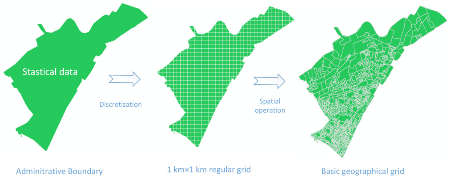
For other data, such as population census data and survey data, data collection was based on administrative districts. Data were discrete, based on regular grids of 1 km × 1 km. The mapping from regular grids to basic grids is created by geographical location, where regular grids were aggregated into irregular basic grids. At last, the data of urban management events and population are referenced to the basic grid system (Figure 4).

2.3. Evaluation Indexes for Community Livability

In a city, a community is an independent object with rich semantics in physical and human urban geography. Meanwhile, the community is also a basic unit of data analysis. A livability index system was therefore constructed from quantifiable dimensions of human needs at the community scale. These dimensions relate to safety, health, convenience, and comfort. Particularly, data availability and quantification are required when constructing a livability index system [24,25]. In our work, 26 indices were identified as shown in a table in Appendix A. The community livability index system is constructed in four dimensions of community management, living environment, facilities and services, and safety.

(1)

Community management

Community management reflects the level of community self-management ability and community service quality, which are implied by residential district level and public service management [26]. There are two indicators in this dimension. The residential district level refers to the class of residential environment, spatial layout, and auxiliary facilities. Public service management implies the community self-organization and management ability and are measured with the number of complaining events from community residents.

(2)

Residential environment

The living environment of a community provides residents with human environment and physical environment, particularly built environment [27,28]. Six indicators are used to quantify the residential environment dimension. The physical environment reflects the status of obligatory living resources, including natural water, noise pollution, greening rate, and industrial pollution. Built environment reflects building quality and indoor conditions, such as floor area ratio and building age.

(3)

Facility services

Facility services, indicating life quality of community residents, consist of facilities related to transportation, commerce, education, sports, and medical infrastructure. Facility services are calculated with 15 indicators. The traffic facilities are concerned with the coverage area of bus stop service, subway station service, and parking lot service [28,29]. Commercial services are mainly divided into convenience store service, supermarket service, and shopping center service. Education services are concerned with kindergartens, primary and secondary schools. Cultural and sports services are concerned with parks, public squares, cultural facilities, and sports facilities. Medical services are concerned with hospitals, clinics, and community health service centers.

(4)

Safety and health

Safety and health start from the resident feelings, reflecting their sense of security in the community and the situation of safety facilities, including community and fire safety [30,31]. Three indicators are used to describe safety and health dimension. Community security includes the proportion of unsafe population, such as prisoners, drug addicts, and the density of electronic monitoring device, whereas fire safety is mainly quantified by the coverage index of the fire station service area.

2.4. Construction of Community Livability Evaluation Model

The evaluation model is used to calculate a livability score for each community. After data cleaning and normalization, the value indexes described as in Section 2.3 are calculated objective weight based on the contribution rate estimated via principal component analysis (PCA), then combined expert scoring to create a comprehensive weight. This comprehensive weight can be used to estimate livability for each grid. These livability scores for grids are aggregated into the community livability value.

2.4.1. Evaluation Index Quantification

Principal component analysis is a typical method of multivariate statistics, simplifying the observed variables. Principal component analysis was used for dimension reduction of 26 indices [32,33]. Through index standardization and PCA dimension reduction, data can be prepared well for the community livability evaluation.

• Index standardization

Before performing the PCA, 26 indices were standardized to eliminate the influence of the redundancy and order of magnitude of the data. Public complaints, noise pollution along the main road network, and industrial pollution are treated as negative indicators. Residential area services and facility services are measured as ordinal data, taking standard scores according to the classification rules [34,35]. The coverage of various public facilities, transport, and the proportion of area covered by lakes were scored with reference to standard values. Building density was quantified by residential plots. The floor area ratio was calculated by gross floor area divide the area of plot. According to the threshold value of 1.8 [35], the score is 100 if the floor area ratio is less than 1.8; in addition, the score was calculated according to the proportion of floor area ratio to 1.8 when the floor area ratio is more than 1.8.

2.

Calculate the correlation matrix Z and covariance matrix R

$$z=\left(\begin{array}{cccc}{z}_{11}& z_{12}& \dots & z_{1p}\\ z_{21}& \dots & \dots & z_{2p}\\ \dots & \dots & \dots & \dots \\ z_{n1}& z_{n2}& \dots & z_{np}\end{array}\right),$$

(6)

Denoted as the correlation matrix Z (z_ij), is the correlation matrix of standardized indicator variables X_i and X_j (i, j = 1, 2, …, p). The correlation matrix Z is transformed into the covariance matrix R, denoted as [r_ij]_p*p. r_ij referred to the covariance of the variable z_i and z_j. Both matrices have the characteristics of real-value and symmetry, (z_ij = z_ji) and (r_ij = r_ji).

$$r_{ij}=\frac{{\displaystyle \sum _{k=1}^n(z_{ki}-{\overline{z}}_i)(z_{kj}-{\overline{z}}_j)}}{\sqrt{{\displaystyle \sum _{k=1}^n{(z_{ki}-{\overline{z}}_i)}^2{\displaystyle \sum _{k=1}^n{(z_{kj}-{\overline{z}}_j)}^2}}}}$$

(7)

3.

From the covariance matrix R, the eigenvalues $\mathsf{\lambda }$ and eigenvectors e_ij are calculated by factor analysis of Statistical Product and Service Solutions (SPSS). The principal component contribution rate M_i and cumulative contribution rates N_i are calculated by extraction of factor analysis of SPSS. As the cumulative contribution rate of the eigenvalues is 85–95%, correspondingly 18 principal components are selected.

$${\mathrm{N}}_i=\frac{{\displaystyle \sum _{k=1}^i{\lambda }_k}}{{\displaystyle \sum _{k=1}^p{\lambda }_k}}(i=1,2,\dots ,p),$$

(8)

2.4.2. Determine the Comprehensive Weight

The subjective and objective weights were combined into a comprehensive weight for livability evaluation. The objective weight has been calculated according to the cumulative contribution rate and eigenvector of principal component analysis.

$${\mathrm{L}}_i={\displaystyle {\sum }_{k=1}^{18}{\mathrm{N}}_{\mathrm{K}}\ast {\mathrm{e}}_{\mathit{ki}}}.$$

(9)

Here N_K has been calculated as the kth cumulative contribution rate and e_ki has been represented the ith component of the kth eigenvector.

The subjective weight ${\mathsf{\omega }}_i$ takes a value with reference to Chinese scientific evaluation standard of livable cities, expert experience and data quality. They were determined by expert consultation. Five experts familiar with the development and environment protection actual situation of Wuhan were invited to discuss and decide the weight value for each index from environmental, geography, public management aspects. The following expression is used to determine the comprehensive weight:

$${\mathrm{J}}_i=\mathsf{\alpha }\ast {\mathrm{l}}_i+(1-\mathsf{\alpha })\ast {\mathsf{\omega }}_i,$$

(10)

where l_i is the objective weight, α is the adjustment ratio of objective weight and subjective weight, and (1 − α) is the proportion of subjective weight. Normally, the subjective and objective weights are equal, and α equals 0.5 by default [36]. According to the experimental data statistical results in the previous literature [30], livability is positively correlated with urban housing prices. In our study, α is an experience value depending on whether the scores of livability is conformed with the house price and public experience. Therefore, this study takes α = 0.8 to calculate the comprehensive weight.

2.4.3. Calculation of Livability Score

After acquiring the standardized data and comprehensive weights for each index in Section 2.4.1 and Section 2.4.2, the livability scores of each grid F_k were calculated. In addition, the livability score for a community was obtained under the considerations of grid score C and its proportion for the total area of the community.

Let the k-th grid score be

$$F_k={\displaystyle {\sum }_{i=1}^p}{Z}_i{}_k\ast {\mathrm{J}}_i,$$

(11)

Assume that n grids exist in a community, the area of the community is S, the area of the kth grid is S_k, and grid score is F_k, then the community livability score C is as follows:

$$C={\displaystyle {\sum }_{k=1}^n(S_k/S)\ast F_k}.$$

(12)

Similarly, the livability scores of all communities in the study area are obtained.

3. Results

The basic geographical grid system is the crucial part of our work. It can be regarded as irregular division of geographical space concerning community boundaries and multiple constraints. All kinds of big data from governmental information systems were spatially aggregated with basic geographical grids for livability evaluation. The results of livability index and livability score showed the effectiveness of basic geographical grids on the community livability evaluation.

3.1. Space Partition: Basic Grids

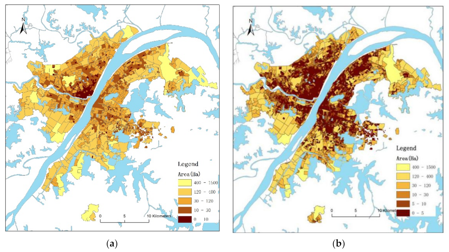
Figure 5 compared the spatial distribution of community and basic grids, displaying the results of partition of 916 communities into 7702 basic grids in the study area.

As Shown in Figure 5a, the spatial distribution of communities included small size communities clustered in the center and large size communities located in the peripheral area. According to

Table 2. Number and size of communities and basic geographical grids.

Area Range of Communities (ha)	Number	Proportion	Area Range of Grids (ha)	Number	Proportion
0–10	168	18.34%	0–5	6462	83.90%
10–30	353	38.54%	5–10	571	7.41%
30–120	286	31.22%	10–30	391	5.08%
120–400	93	10.15%	30–120	192	2.49%
over 400	16	1.75%	120–400	78	1.01%
			over 400	8	0.10%

, 56.7% of the communities covered an area of less than 30 hectares, which were distributed along Yangtze and Hanjiang river banks, the central area of Hankou, and the Wuluo road of Wuchang district, but 11.9% of the communities covered an area of more than 120 hectares, which were distributed in the peripheral of the city. Among them, the largest community was the WISCO community located in the WISCO plant of Qingshan District, covering an area of 1499.49 hectares. The smallest community was the Nanhu Yayuan community located in Hongshan street of Hongshan District, covering an area of 0.2186 hectares. Communities of different sizes would affect the spatial difference of grid.

The communities were different in basic geographical grids. Figure 5b showed that smaller grids were concentrated in small size and medium sized communities. In terms of the grid size (Table 2), the size of 96% basic grid cells was less than 30 hectares, and one community was partitioned into 8.4 grids on average. The largest grid was the Wuhan Iron and Steel (Group) Company (WISC) community of the WISC plant in Qingshan District, where the whole community was one grid cell. The smallest grid was located in Hualou street covering an area of 0.0528 hectares. The grid cells less than 30 hectares were not only distributed along the Yangtze and Hanjiang river banks, the central area of Hankou, and along Wuluo Road, but also near Gusaoshu, South Lake, and the Optical Valley area. It can be seen that the partitioned grid could be transformed from any management grid with spatial constraints, so as to describe the subtle changes of community inner space.

3.2. Results of Community Livability Index

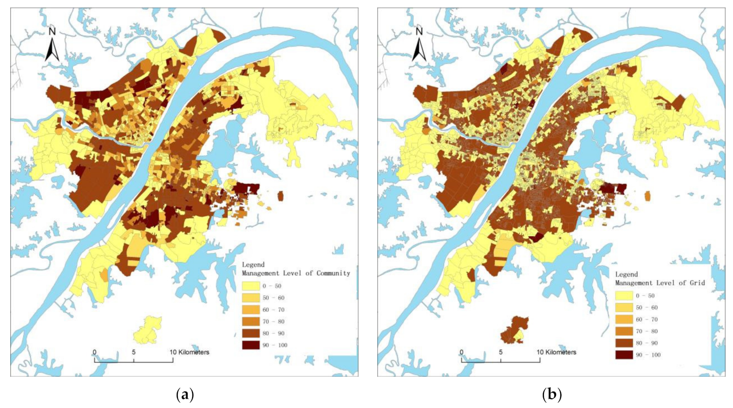
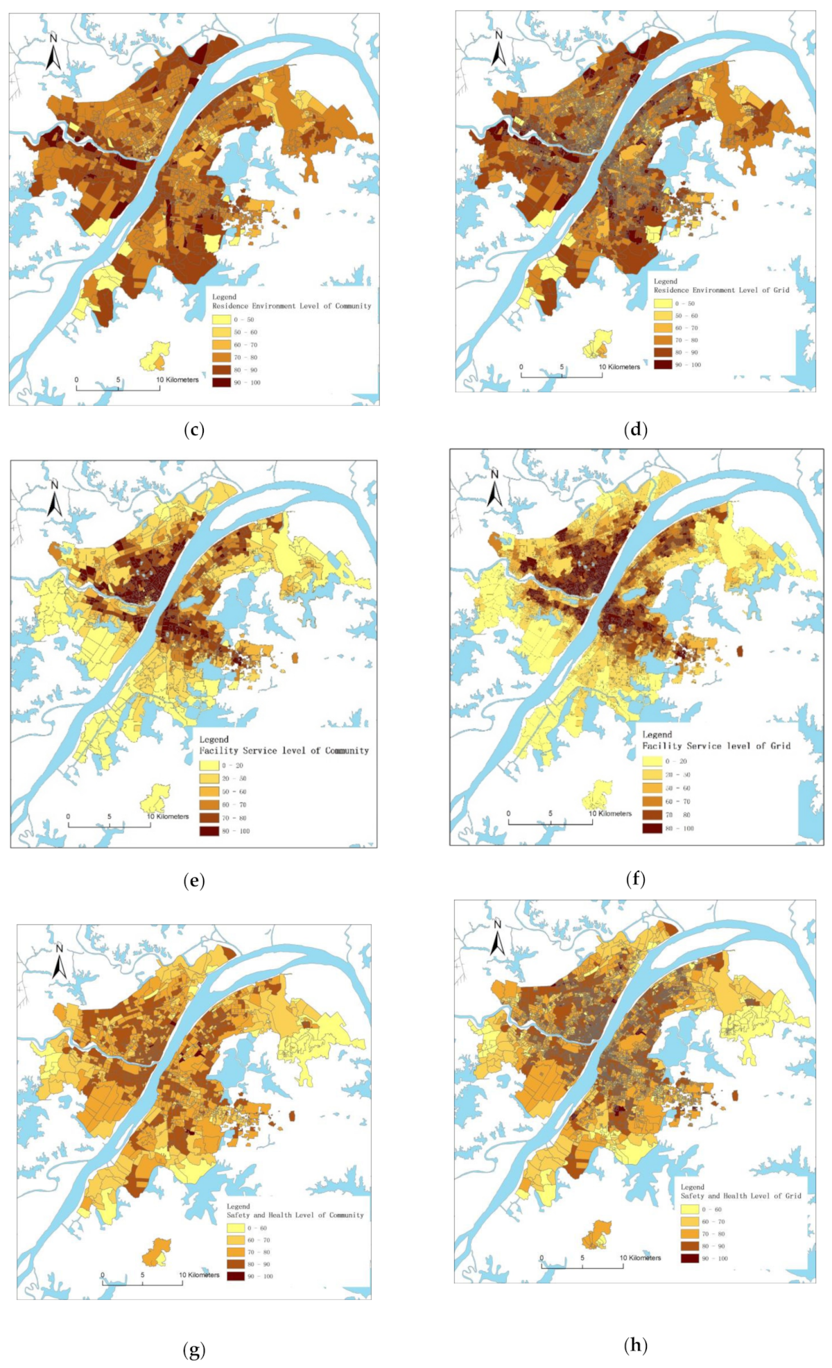
Figure 6 shows the spatial distribution of the calculation results of community management, residence environment, facility services, safety, and health index at the community and basic grid scales separately. Figure 6b,d,f,h is graphed by the calculation of indices of 18 principal components by grids. Figure 6a,c,e,g is aggregated into the community livability score by weighting the grid values. The weight values of each index are used for the calculation of livability (Appendix B).

In Figure 6a,b, there was obvious spatial heterogeneity in the scores of community management index at grid scale. Correspondingly, the high scores distribution at the community scale were consistent with the high score distribution at the grid scale. Most of them were aggregated in the large-scale community in the northern peripheral area of Hankou, the new community along the Yangtze river bank in Wuchang, the new community along the Yangtze River bank in Nanhu area of Wuchang and Yongfeng area of Hanyang. In Figure 6c,d, the residence environment index score was mainly 60–80. The spatial distribution of high scores was relatively uniform at the scales of both community and grid. The similarity distribution implies that the residence environment is greatly affected by geographical location and the water system, and is little affected by the grid size. In Figure 6e,f, the communities with facilities services index over 60 were mainly distributed along the Yangtze river bank in Hankou, Qintai Avenue in Hanyang, and Wuluo road in Wuchang. In general, the communities with complete facility services were symmetrically distributed along the Yangtze river bank, showing the L-shape pattern. This result indicates that the clustering trend of facilities in the urban center is consistent with the axis of urban expansion. In Figure 6g,h the average score of safety and health index was 60–80, and the spatial distribution of safety and health was relatively uniform. Overall, the spatial heterogeneity of community livability, especially concerning residence level, safety, and health level, was explored by gridded data mapping.

3.3. Evaluation of Community Livability

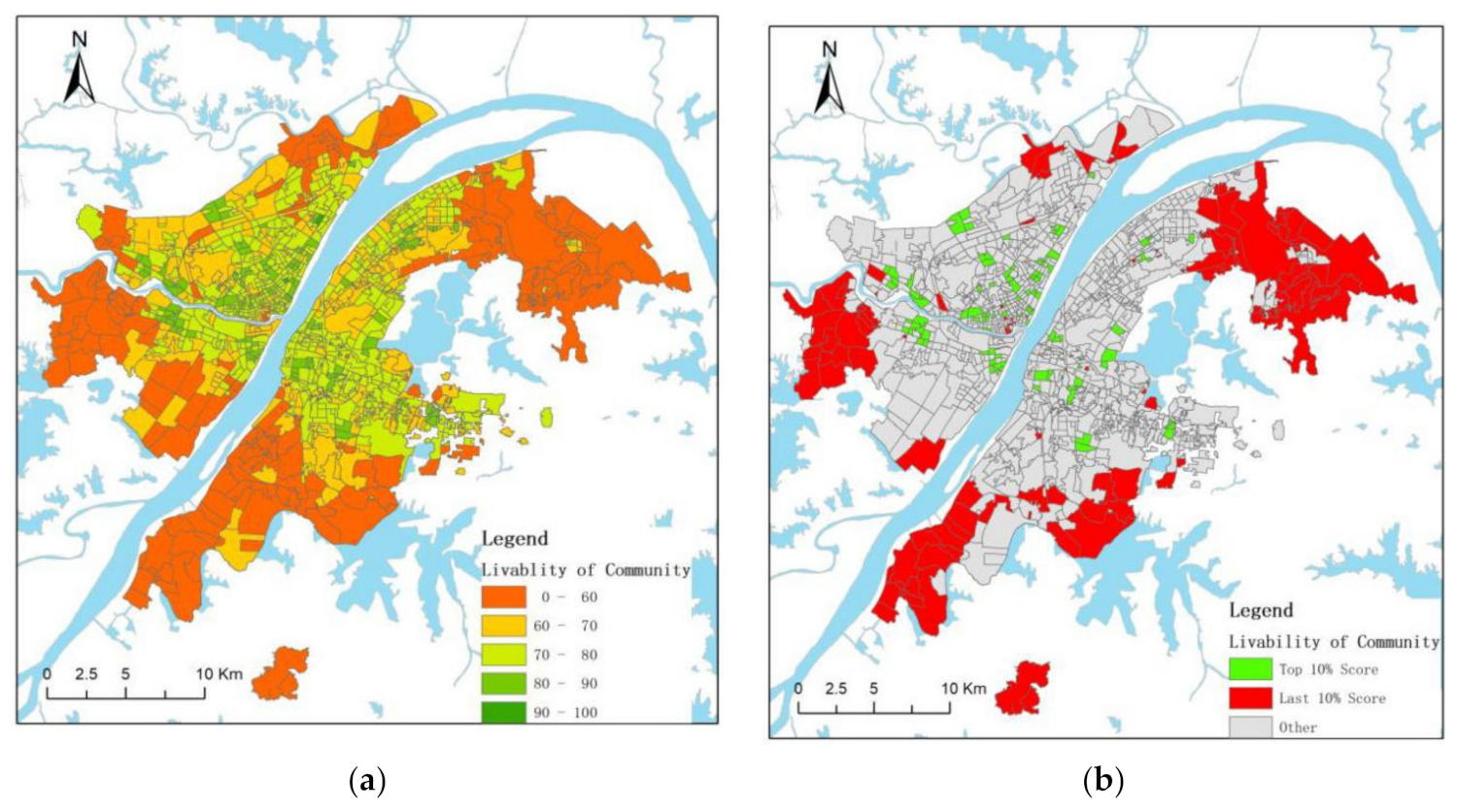
Figure 7 introduces the results of community livability evaluation and explores the spatial distribution of community livability scores (Figure 8).

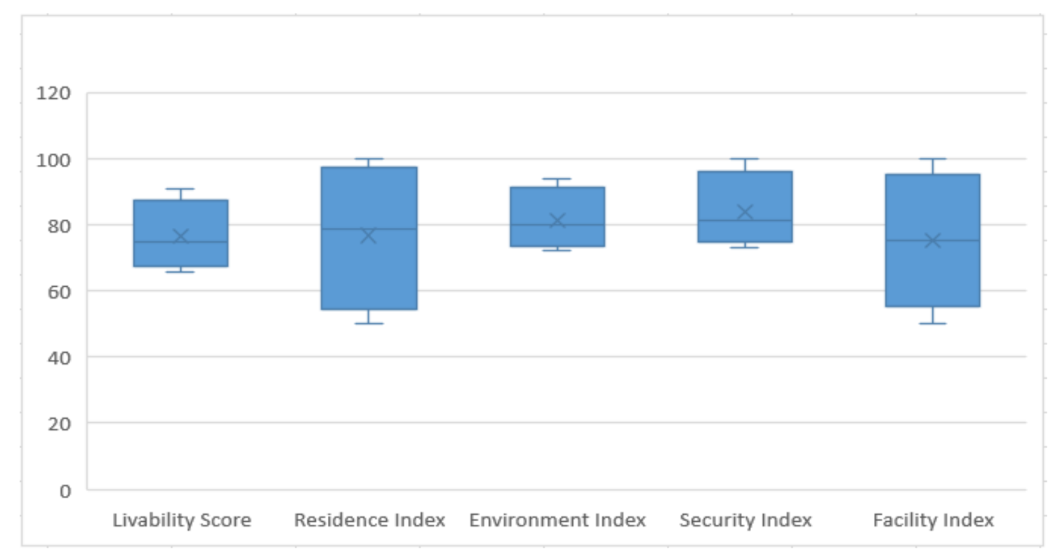
According to Figure 7a, the distribution of community livability scores is unbalanced, and owns the “cross” feature of decreasing from the center to periphery. Medium and high livable scores clustered along the river bank in the central region, but not clustered in areas of sufficient water resources. There is a spatial pattern on the main axis of urban development and the business circle along the river bank. On the contrary, the areas with poor livability is less surrounded with physical environment, and are mainly distributed in the chemical industry zones on the city peripheral. Moreover, these communities have poor housing conditions, old aging population, many dangerous buildings, insufficient facilities. Thus, the spatial distribution is relatively random. In Figure 7b, communities of livability high scores are not clustered in the central area, but evenly distributed around the second ring road. Communities of livability low scores are obviously clustered, such as Wugang community of Qingshan District, Yongfeng street of Hanyang District and Zhangjiawan Street of Hongshan District. Apart from the overall trend (

Table 3. Overall and dimension assessment scores of community livability.

	Min	Median	Quartile	Max	Average	Std
Overall Livability	66	72.62	77.19	90.84	67.68	17.51
Residence Index	50	67.02	90	100	64.03	24.52
Environment Index	72	76.62	82.92	93.85	74.49	16.74
Security Index	73	79.37	83.34	100	77.76	8.88
Facility index	50	69.94	80.20	99.93	62.10	25.81

), Figure 8 shows that the residential management level and facility service level vary widely in the region. In general, communities of high and relatively high livability scores are distributed along Yangzi and Hanjiang river banks. Meanwhile, communities of low livability scores, being with polycentric and lumpy features, are located on the city peripheral.

4. Analysis and Discussion

The purpose of this study is generating a set of basic geographic grids for data connections between irregularly shaped management boundaries, and further evaluating the community status of economic development, living environment, convenience, safety, and health. Therefore, space partitioning into basic grids was proposed for aggregating government data of overlapping management boundaries. The set of basic grids is used for community livability evaluation with weighted summarization of grid scores based on the data of Wuhan. As a result, it is found that the fragmentation degree of basic geographical grids is increasing along the intersection of two rivers. This grid partition impacts the management, environment, facilities and security of the community, and then affects the livability score of the community.

4.1. Spatial Pattern

The results of geostatistical analysis of indexes for each dimension is useful to prove statistically the spatial pattern of community management, physical environment, public facility and security found by the visualization in Section 3. Since the livability is affected by the distance from the community to the city center and related to the surrounding communities, two spatial relationship conceptual models of inverse distance and continuity edges and corners are selected to generalize the spatial model of community. An inverse distance model is suitable to analyze community features while the nearby neighboring community have a larger influence on the computations for a target community. Continuity edges and corners model is adaptive for calculating community polygon feature, on account of influence by community sharing a boundary, or a node. Using ArcGIS 10.3 software to analyze global spatial autocorrelation of evaluation index for each dimension. The spatial pattern analyzed by the spatial autocorrelation tool can diagnoses whether the evaluation scores are cluster or not.

Table 4. Global spatial autocorrelation of community livability.

Livability Dimension	Spatial Relationships Modeling	Moran’s I Index	Z-Score	p-Value	Spatial Pattern
Residence management index	Inverse Distance	0.13	17.34	0	Clustered
Residence management index	Continuity edges and corners	0.30	15.76	0	Clustered
Environment index	Inverse Distance	0.05	7.20	0	Clustered
Environment index	Continuity edges and corners	0.05	7.20	0	Clustered
Facility index	Inverse Distance	0.06	7.72	0	Clustered
Facility index	Continuity edges and corners	0.08	4.39	0	Clustered
Security index	Inverse Distance	0.28	37.14	0	Clustered
Security index	Continuity edges and corners	0.44	23.56	0	Clustered

shows Moran’s I value of global autocorrelation in all four dimensions of community livability. It reveals positive spatial autocorrelation in both spatial modeling statistically. The P-value associated with Z-scores of eight indexes prove that the pattern is significant at the 99% confidence level (Table 4). Overall, these four dimensions were clustered statistically in space. Obviously, the spatial autocorrelation of residence management index and security index are higher than the other two dimensions based on the spatial relationship model of continuity edges and corners.

Furthermore, statistical results of Anselin local Moran’s I in Figure 9 have been executed to explore the spatial clustering pattern of these four dimensions. From the results, there are obviously high-value clusters and low-value clusters in community residence and community safety, which is consistent with the conclusion in Table 2. On the contrary, there is no obvious spatial clustering phenomenon in human settlements and facility services. It reveals that the spatial heterogeneity of community management needs and community security needs can be easily quantified by the indicators, while the clustering pattern of residential environment needs and public facility needs is explored weakly. Specific to the dimension of community management, the heterogeneity of the index is reflected in the construction year of the community, the scale, and the property management quality. High-value clusters are concentrated in Tazi Lake, Sixin area, Nanhu area, and residential areas near East Lake. These communities are newly built residential groups with a large area in dense grids and standardized property management. Low-value clusters are in communities such as Wuhan Iron and Steel, Qingling Township. These communities are old communities in sparse grids, insufficient public facilities, and non-closed management. It is necessary to strengthen community quality and property services. In the dimension of community security, security indicators are related to the density of the grid and the number of security devices. In Figure 9d, the security index showed high-high clustering in the center of Hankou, Hanyang, and Wuchang near the Yangtze River Bridge, and low-low clustering in urban fringe communities. To explain this phenomenon, central communities in large populations required more security monitoring devices to help to analyze and predict security events. Meanwhile, the urban fringe communities in a small population are normally required in fewer security devices and sparse grid partition. In the dimensions of human residence and facility service, the phenomenon of spatial clustering is not obvious (Figure 9a,c). Although the high values of the residential environment index and facility service index are in similar distribution (Figure 9b,c), the heterogeneous and the cluster effect in the living environment and facility resource allocation of the communities are not significant. According to the low Moran’s I value in Table 4, it proves that residential conditions and facilities in the study area are matched with residential demand in balance. In a sense, the spatial pattern of four dimensions helps to explain the mismatch of residential needs and community life at grid scale. This method fit to qualify the spatial difference in residential and security dimensions than environment and public facility dimensions.

4.2. Spatial Heterogeneity of Community Livability

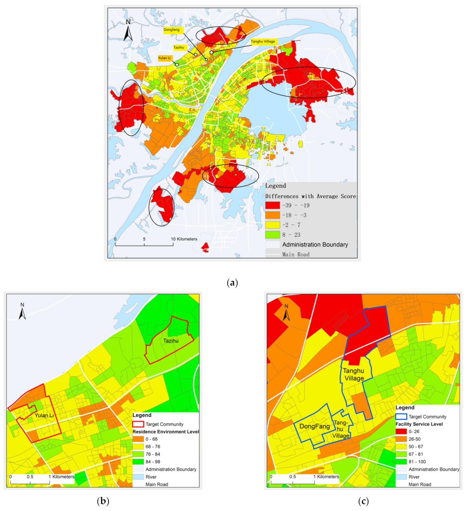
Judging from the evaluation results of community livability (Figure 7), this grid-based modeling method can analyze the spatial differences in resource allocation, land use situation, and population within the community. As shown in Figure 10a, the spatial differences between community livability scores and average livable scores were apparent. According to resource allocation, the community is divided into several internal plots by grid boundary, and their ability to obtain surrounding public service facilities is different (Figure 10). On one hand, this difference is affected by the different locations of the community itself and the uneven distribution of public service facilities. For example, in Figure 10b the residential area in the Yulanli community locates in a large residential group with sufficient shopping, education, and public facility, so the overall level of resource allocation is 85.5. Only seldom plots in this community are around 64.2 in facility service level. Figure 10b shows the comparison of residence environment by grids in the Yulan Li community and the Tazihu community. Residence environment scores in grids vary from 0–76 in the Yulan Li community while it varies from 76 to 97 in the Tazihu community. On the contrary, Yuejin and Tazihu communities in Yangcha Lake residential group lack education and medical facilities, and the level of resource allocation is around 38.9. On the other hand, the level of public service facilities in the plots within the community is related to the size of the community. From the same location, communities in a large area are more liable to access facilities such as hospitals, shopping centers, and public transportation. Such as in Figure 10c, in the same Houhu area, the service level of grids in the Dongfang community of 50 ha varies from 50–70, while the service level of grids in the Tanghu Village community of 170 ha spans 4 levels from 20 to 60. This is due to the increase of the matching difference between the internal plots of the community and the adjacent resources while the area of community increases. It can be seen that using grid cells smaller than the community to measure the level of resource allocation is better to reflect the availability of public facilities in the community.

From the perspective of land use, the livability of the community is affected by the interactions with the environment, public facilities, and transportation by its land function. Compared with communities located in residential land, communities in industrial land are larger in area and scale, less public facilities, and have lower quality of community management level due to different functional positions (Figure 10a). For example, the levels of public transportation, shopping, primary and secondary school facilities, and medical service in the Qingshan Industrial Zone and the Yingwuzhou Industrial Zone, which were circled in Figure 10a are lower than those in the residential group area around rivers and lakes. Thus, the livability based on the analysis of the internal plots of the community will reveal the differences in community functions.

Thirdly, the livability based on community plots in Wuhan can reflect the population differences within the community. In China, communities range from thousands to tens of thousands of people. For large communities, the population is large and the population characteristics of the inner plots are diverse. High-income young people prefer to live in neighborhoods with convenient commutes and well-equipped facilities. The inner livability of the community in Figure 10 will support the study of how the population affects livability further. From the above three aspects, it can be seen that the evaluation of a livability-based grid method is suitable to analyze the association between the community inner and the surrounding urban elements in the spatial location, land use nature, population, and other dimensions.

4.3. Validation and Uncertainty

The sensitivity of community livability scores is varying with domain-specific semantics, spatial shape, and spatial scales [37,38].

(1)

Validation of grouping communities. The uncertainty of community livability evaluation exists in multiple aspects of index system, index scores, evaluation, data accuracy, data standardization, weighting. To test the truth of livability evaluation, we perform field surveying about the grouping communities of high, middle, and low livability scores (

Table 5. Field surveying about grouping communities.

Community Name	livability Score	Area (Ha)	Grid	Population Density (Person/ha)	Community Surveyed
Wuhan Xintiandi Community	87.39	36	10	120.7	The high-class community built in 2009, adjacent to Jiangtan park and multi-functional commercial facilities. It is close to 2 subway lines, 13 primary and secondary schools and 1 Grade-A hospital.
Island Community	76.70	25.9	5	137.28	The Island community is an ordinary community built in 2002 with a good landscape, a floor area ratio of 1.05, and a greening rate of 45%. It is close to three subway stations, primary and secondary schools, and hospitals.
Danshuichi Village Community	74.9	141.9	2	57.38	This community is a general residential area built in 2004, including 396 buildings. The accessibility of facilities meets the daily need, but it lacks primary and secondary education facilities and large hospitals.
Wuyi Community	29.1	30.6	1	25.12	The Wuyi community is located in Qingshan District, the village in the city formed in 1997. There is a serious shortage of cultural, educational and commercial facilities and inconvenient transport while obvious air pollution problem.

).

(2)

Spatial scale effects. Moreover, the modifiable area unit problem (MAUP) exists objectively [38]. Following that, the evaluation results of grid- and community-scales in Figure 5 show that granularity and partition affect the livability scores. Multiple scales or the optimal scale of data and analysis are in demand.

4.4. Overall Comparison and Advantages

Community livability offers a means of analyzing the interaction between humans and the environment, and further improving urban living quality. We have partitioned space into a set of basic grids. The basic grid is smaller than the community and is helpful to construct the community livability evaluation model. Firstly, the small scale grid analysis of livability clarifies more structural details of community livability. Using a community for livability evaluation, the livability results may not be at high precision [39]. For example, few communities near the lake and the river are livable [23]. Evaluation based on the grid can increase the differentiation degree of livable results and reflect the index of different plots in the community. Secondly, the subjective and objective weights given on the grid are flexibly used for evaluating community livability. These weights are not absolute livability standards. However, it reflects the coordination of resources within the community by considering the internal land use relationship, spatial partition, and data availability. Using these combined weights is helpful to track and find the shortboard of the community in time. Thirdly, the evaluation model meets the data requirement of accuracy, granularity, and effectiveness. Previous studies used remote sensing images, POI data, and statistical data to calculate the livability index [18]. By the influence of data source and data processing methods, these results showed some deviation. However, this study handles big data from different governmental information systems, resulting in higher data accuracy and reliability in community livability evaluation. This method is more suitable for application and promotion to other cities.

Our results are approximately consistent with the studies [30,40]. The spatial distribution of community livability shows the mode of “low outside and high inside”. The high livability and low livability communities are medium size communities. In Wuhan, the high livability communities are mostly distributed along the two river banks, and Luoyu road extending into the Optical Valley. The difference from other studies is that no clustering effect is found in Wuhan’s residential environment and public facilities service level, otherwise spatial aggregation is revealed in community management, safety, and health. In the case of Wuhan, this method is sensitive to examine livable in community management and security.

5. Conclusions

This study proposes an approach to integrating government spatial data, POI, and other multisource data. Through space partitioning into basic grids and the index system construction of community livability, 26 livability index data are extracted for practically evaluating the livability of community management, residence environment, facilities service, and safety and health in Section 2.2.2. Taking Wuhan as an example, the feasibility and effectiveness of a basic grid system or space partition experiment in community livability evaluation. Compared with the studies of community livability in Section 1, this paper introduces the concept of a basic geographical grid and proposes an evaluation method based on integrating multi-source data of population, land, housing, and public facilities of multiple professional grids. It helps to reduce data deviation and promote government geographic information in the application of social governance, urban optimization, building 15 min of life circles. The conclusions are as follows:

(1)

The basic grid organizes and integrates the data of various management semantics in a smart city. It expresses the differences in public facilities and resources configuration needs within communities. Judging from the results of livability evaluation, this method is sensitive for revealing the potential short come and demands of public resources and services within community boundaries and provides a feasible technical method for urban modernization governance. Based on the study of Wuhan, it provides technical routes and experiences for more areas to integrate government data, improving the accuracy and time-efficiency of livability evaluation.

(2)

Urban basic grid partition helps to identify the spatial pattern of livability from the difference within the community. From the results, spatial cluster of community livability is at the 99% confidence level by Z value > 2.58, p-value < 0.01. According to the four dimensions, community management and safety and health have obvious high-value clusters and low-value clusters separately, while the residential environment and facility service have no obvious spatial cluster phenomenon in Figure 8. The spatial heterogeneity of livability was affected by location, facility service, and size of the grids.

(3)

The overall livability of the study area is good by the average livability index of 67.68. The quality of the environment and security dimension were better than those of residence and facility dimension by the score at 74.49 and 77.76. 33.5% of communities were over average livability score and were located in the center of the study area. Surrounding areas in poor livability mainly expose the lack of livability of communities located in industrial areas. Factors’ effects on community livability need more discussion.

References

1. Fang, C.; Yu, D. China’s New Urbanization: Developmental Paths, Blueprints and Patterns; Springer and Science Press Ltd.: Berlin/Heidelberg, Germany, 2016; pp. 14–18. [Google Scholar] [CrossRef]
2. International Institute for Sustainable Development. Sustainable Development Goals Report 2020; Department of Economic and Social Affairs Press: New York, NY, USA, 2021; pp. 46–47. [Google Scholar]
3. Zhan, D.; Kwan, M.P.; Zhang, W.; Fan, J.; Yu, J.; Dang, Y. Assessment and determinants of satisfaction with urban livability in China. Cities 2018, 79, 92–101. [Google Scholar] [CrossRef]
4. Zhang, W.Z. Index system and method of residential environmental evaluation in inner cities. Sci. Geogr. Sin. 2007, 27, 17–23. [Google Scholar]
5. Howard, E. Garden Cities of Tomorrow; Swan Sonnenschein & Co Ltd.: London, UK, 1902; p. 26. [Google Scholar] [CrossRef]
6. Kashef, M. Urban livability across disciplinary and professional boundaries. Front. Archit. Res. 2016, 5, 239–253. [Google Scholar] [CrossRef] [Green Version]
7. Giannousopoulou, M.I. Enhancing the livability of urban blocks by assessing and improving the microclimate in the Mediterranean: The case of Peristeri, Athens. Master Thesis, HafenCity University Hamburg, Hamburg, Germany, 2016. [Google Scholar]
8. Norouzian-Maleki, S.; Bell, S.; Hosseini, S.B.; Faizi, M. Developing and testing a framework for the assessment of neighbourhood livability in two contrasting countries: Iran and Estonia. Ecol. Indic. 2015, 48, 263–271. [Google Scholar] [CrossRef] [Green Version]
9. AtKisson, A. Developing indicators of sustainable community: Lessons from sustainable Seattle. Environ. Impact Assess. Rev. 1996, 16, 337–350. [Google Scholar] [CrossRef]
10. Khorasani, M.; Zarghamfard, M. Analyzing the Impacts of Spatial Factors on Livability of Peri-Urban Villages. Soc. Indic. Res. Int. Interdiscip. J. Qual. Life Meas 2018, 136, 693–717. [Google Scholar] [CrossRef]
11. Wei, Z.; Chiu, R.L.H. Livability of subsidized housing estates in marketized socialist China: An institutional interpretation. Cities. 2018, 83, 108–117. [Google Scholar] [CrossRef]
12. Li, S.; Yang, Z.Z. The contents and index system of evaluating livable community for urban elderly. Northwest. Popul. 2012, 33, 17–21. [Google Scholar]
13. Miller, H.J.; Witlox, F.; Tribby, C.P. Developing context-sensitive livability indicators for transportation planning: A measurement framework. J. Transp. Geography. 2013, 26, 51–64. [Google Scholar] [CrossRef] [Green Version]
14. Onnom, W.; Tripathi, N.; Nitivattananon, V.; Ninsawat, S. Development of a liveable city index (LCI) using multi criteria geospatial modelling for medium class cities in developing countries. Sustainability 2018, 10, 520. [Google Scholar] [CrossRef] [Green Version]
15. Lu, J. Building a New Community: A Study of Community Governance in Chinese Cities; Peking University Press: Beijing, China, 2019; pp. 136–138. [Google Scholar]
16. Zhang, W.Z. Theoretical research of the livable city construction and its practice reflection in China. Urban Plan. Int. 2016, 31, 1–6. [Google Scholar] [CrossRef]
17. Khorrami, Z.; Ye, T.; Sadatmoosavi, A. The Indicators and Methods used for Measuring Urban Liveability: A Scoping Review. Rev. Environ. Health 2021, 36. [Google Scholar] [CrossRef]
18. Zhang, Y.; Li, Q.Z.; Wang, H.Y.; Du, X.; Huang, H.P. Community scale livability evaluation integrating remote sensing, surface observation and geospatial big data. Int. J. Appl. Earth Obs. Geoinf. 2019, 80, 173–186. [Google Scholar] [CrossRef]
19. Zhang, W.Z.; He, J.; Chen, L. Method System of Urban Physical Examination for High Quality Development in China. Sci. Geogr. Sin. 2021, 41, 1–12. [Google Scholar]
20. Chen, J.P.; Zhang, Y.; Yu, Y.J. Effect of MAUP in spatial autocorrelation. Acta A Geogr. Sin. 2011, 66, 1597–1606. [Google Scholar]
21. Wuhan Natural Resources and Planning Bureau. Wuhan 2049 Long-Term Development Strategic Plan; People’s Government of Wuhan City: Wuhan, China, 2014. [Google Scholar]
22. Wuhan Bureau of Statistics. Wuhan Statistical Book 2020; Wuhan Bureau of Statistics: Wuhan, China, 2020. Available online: http://tjj.wuhan.gov.cn/ (accessed on 1 November 2021).
23. Li, D.R.; Zhu, X.Y.; Gong, J.Y. From digital map to spatial information on grid: Thoughts on multi-level grid theory of spatial information. J. Wuhan Univ. (Inf. Sci. Ed.) 2003, 28, 642–650. [Google Scholar] [CrossRef]
24. Ballas, D.; Tranmer, M. Happy people or happy places? A multi-level modelling approach to the analysis of happiness and well-being. Int. Reg. Sci. Rev. 2012, 35, 70–102. [Google Scholar] [CrossRef]
25. China Urban Science Research Association. Livable City Chinese Scientific Evaluation Standard; China Urban Science Research Association: Beijing, China, 2007. [Google Scholar]
26. Komeily, A.; Srinivasan, R.S. A need for balanced approach to neighborhood sustainability assessments: A critical review and analysis. Sustain. Cities Soc. 2015, 18, 32–43. [Google Scholar] [CrossRef]
27. Wagner, F.; Caves, R. Community Livability: Issues and Approaches to Sustaining the Well-Being of People and Communities; Routledge: London, UK, 2012. [Google Scholar] [CrossRef]
28. Long, Y.; Li, M.Y.; Li, J. Monitoring built environment of China with new data: Indicator system and case studies. Urban Dev. Stud. 2018, 25, 86–96. [Google Scholar]
29. Giap, T.K.; Thye, W.W.; Aw, G. A new approach to measuring the livability of cities: The global livable cities index. World Rev. Sci. Technol. Sustain. Dev. 2014, 11, 176–196. [Google Scholar] [CrossRef] [Green Version]
30. Peng, K.; Zhang, K.; Yan, H.H. Construction of evaluation index system of livable community in Wuhan based on multidisciplinary evaluation perspective. Urban. Archit. 2017, 26, 70–72. [Google Scholar]
31. Arifwidodo, S.D.; Perera, R. Quality of life and compact development policies in Bandung, Indonesia. Appl. Res. Qual. Life 2011, 6, 159–179. [Google Scholar] [CrossRef]
32. Govindan, K.; Rajendran, S.; Sarkis, J.; Murugesan, P. Multi criteria decision making approaches for green supplier evaluation and selection: A literature review. J. Clean. Prod. 2015, 98, 66–83. [Google Scholar] [CrossRef]
33. Guangdong Bureau of Quality and Technical Supervision. Evaluation for the Construction of a Livable Community; DB44/T 1577-2015; Guangdong Bureau of Quality and Technical Supervision: Guangdong, China, 2015; pp. 1–2. [Google Scholar]
34. Office of the Leading Group for the First National Geographical Census of the State Council. Contents and Indicators of National Geoinformation Survey; Surveying and Mapping Press: Beijing, China, 2013. [Google Scholar]
35. Ministry of Housing and Urban-Rural Development of the People’s Republic of China. Standard for Urban Residential Area Planning and Design; GB 50180-2018; China Architecture & Building Press: Beijing, China, 2018. [Google Scholar]
36. Zhu, L.K.; Guo, Y.Y.; Zhang, C.; Meng, J.J.; Ju, L.; Zhang, Y.S.; Tang, W.X. Assessing community-level livability using combined remote sensing and Internet-based big geospatial data. Remote Sens. 2020, 12, 4026. [Google Scholar] [CrossRef]
37. Feizizadeh, B.; Jankowski, P.; Blaschke, T. A GIS based spatially-explicit sensitivity and uncertainty analysis approach for multi-criteria decision analysis. Comput. Geosci. 2014, 64, 81–95. [Google Scholar] [CrossRef] [PubMed] [Green Version]
38. Kwan, M.P. How GIS can help address the uncertain geographic context problem in social science research. Ann. GIS 2012, 18, 245–255. [Google Scholar] [CrossRef]
39. Chen Zeng Song, Y.; He, Q.S.; Shen, F.X. Spatially explicit assessment on urban vitality: Case studies in Chicago and Wuhan. Sustain. Cities Soc. 2018, 40, 296–306. [Google Scholar] [CrossRef]
40. Min, L.; Xiong, B.N. Livable neighborhood planning strategies: Wuhan case. Planners 2012, 28, 18–23. [Google Scholar]
Figure 1. Study area mapping. (a) The central urban area in Wuhan; (b)The distribution of communities in the study area.
Ijgi 11 00038 g001
Figure 2. An approach to community livability evaluation mainly using gridded basic urban geographical data.
Ijgi 11 00038 g002
Figure 3. Domain-specific urban grids: (a) Urban management grid. The purple boundary represents the responsibility area of urban management law enforcement, relating to city image and sanitation; (b) Industrial and commercial administration grid. The dark green boundary represents the responsibility area of market supervision and administration, relating with market entities; (c) Environment protection grid. The blue boundary represents the responsibility area of environment supervision and environmental pollution control. (d) Food and medical quality monitoring grid. The dark yellow boundary represents the responsibility area of monitoring the food and medical quality; (e) Overlap of professional grids. Professional grids partition the space into spatial cells.
Ijgi 11 00038 g003
Figure 4. Then, POI data were converted into spatial data in the CGCS2000 coordinate system. The greening rate reflects ratio of green land area to total land area for each community. The text description of community greening rate is crawled from the community web page, and further the community name, community address, and greening rate were extracted. The result data of the greening rate to each community was then produced through cleaning and structural processing.
Ijgi 11 00038 g004
Figure 5. Spatial distribution of community and basic grids: (a) Distribution of community; (b) Distribution of basic geographical grids.
Ijgi 11 00038 g005
Figure 6. Spatial distribution of community livability indexes:(a) Management score of community; (b) Management score of grid; (c) Residence environment score of community; (d) Residence environment score of grid; (e) facility service score of community; (f) facility service score of grid; (g) Safety and health level of community; (h) Safety and health level of grid. (b,d,f,h) are graphed by the index scores of four dimensions calculated with grid data. (a,c,e,g) are graphed by weighted summarization of grid data in (b,d,f,h).
Ijgi 11 00038 g006aIjgi 11 00038 g006b
Figure 7. The spatial distribution of evaluation of community livability: (a) Distribution of community livability score; (b) High-score and low-score distributions. In (a), the red community represents the lower livable score community and the green community represents the high livable score community; (b) shows 10% communities of high scores in green and 10% communities of low scores in red.
Ijgi 11 00038 g007
Figure 8. Overall and dimension scores of community livability: The overall scores range from 70 to 90 and the dimensions scores range from 50–99.3.
Ijgi 11 00038 g008
Figure 9. Spatial pattern of community livability:(a) Hot and cold points of residence; (b) Hot and cold points of environment; (c) Hot and cold points of facility service; (d) Hot and cold points of security. It shows the statistical results of Anselin local Moran’s I by mapping hot and cold points. The black color represents the cluster around the high value, while the blue color represents the cluster around the low value, the yellow color represents the high value surrounded by low values.
Ijgi 11 00038 g009
Figure 10. Spatial heterogeneity of community livability:(a) Differences with the average community livability; (b) Difference of residence environment by grids; (c) Difference of facility service level by grids. (a) shows the distribution of differences between livable score and average score for each community. (b,c) shows the difference of residence environment, facility service level in grids separately.
Ijgi 11 00038 g010