Abstract
The UN 2030 Agenda sets poverty eradication as the primary goal of sustainable development. An accurate measurement of poverty is a critical input to the quality and efficiency of poverty alleviation in rural areas. However, poverty, as a geographical phenomenon, inevitably has a spatial correlation. Neglecting the spatial correlation between areas in poverty measurements will hamper efforts to improve the accuracy of poverty identification and to design policies in truly poor areas. To capture this spatial correlation, this paper proposes a new poverty measurement model based on a neural network, namely, the spatial vector deep neural network (SVDNN), which combines the spatial vector neural network model (SVNN) and the deep neural network (DNN). The SVNN was applied to measure spatial correlation, while the DNN used the SVNN output vector and explanatory variables dataset to measure the multidimensional poverty index (MPI). To determine the optimal spatial correlation structure of SVDNN, this paper compares the model performance of the spatial distance matrix, spatial adjacent matrix and spatial weighted adjacent matrix, selecting the optimal performing spatial distance matrix as the input data set of SVNN. Then, the SVDNN model was used for the MPI measurement of the Yangtze River Economic Belt, after which the results were compared with three baseline models of DNN, the back propagation neural network (BPNN), and artificial neural network (ANN). Experiments demonstrate that the SVDNN model can obtain spatial correlation from the spatial distance dataset between counties and its poverty identification accuracy is better than other baseline models. The spatio-temporal characteristics of MPI measured by SVDNN were also highly consistent with the distribution of urban aggregations and national-level poverty counties in the Yangtze River Economic Belt. The SVDNN model proposed in this paper could effectively improve the accuracy of poverty identification, thus reducing the misallocation of resources in tracking and targeting poverty in developing countries.
1. Introduction
The 2030 Agenda determined that eradicating extreme poverty is still the largest challenge in the world and placed “No poverty” at the top of the 17 Sustainable Development Goals, which demonstrated the determination to eradicate poverty and hunger in all forms and manifestations [1,2]. Poverty alleviation and eradication critically influence the development of the world economy [3,4,5]. Effective poverty alleviation lies in the accurate measurements of poverty, which are also essential for sound poverty alleviation policy and research because such measurements may shape decisions by individual governments about allocating human and material resources and provide the foundation for efforts to understand and track progress toward improving human livelihoods [6,7].
The scarcity of reliable explanatory variables and poverty measurement methods represents a major challenge to poverty identification [8]. Under the influence of the concept of absolute poverty, several researchers indicated that poverty is an inequality [9,10]. The essential explanatory variable for measuring this inequality was basic living materials, such as income and food. The method to measure this inequality is unidimensional measurement. For example, Brady defines poverty as social exclusion and uses Luxembourg income study data to measure the poverty index of advanced capitalist countries [11].
With the increasing complexity of social poverty, this inequality represented by poverty is increasing correspondingly, such as personal capability [12,13], physiological heath [14], economic well-being [15] and policy formulation [16]. The 2030 Agenda also emphasized the importance of multidimensional understanding of poverty [1]. Therefore, the hypothesis of absolute poverty measured based on basic living materials has been questioned by researchers [4,17]. Poverty, which is also related to health, education, capability and other factors, is multidimensional. The understanding of poverty has also surpassed the absolute poverty represented by basic living materials to multidimensional poverty involving multidimensional variables [18,19]. The poverty measurement method has changed from a unidimensional measurement to a multidimensional measurement [20].
Various approaches for the measurement of multidimensional poverty do exist; among them, A–F double cutoffs [21], Foster–Greer–Thorbecke [22] and first-order dominance [23] have been widely used. In the context of the generalized Alkire–Foster measurement, Bennett revealed the relative poverty state in India, which is not otherwise captured by the traditional unidimensional method [24]. Nowak modified the Alkire–Foster identification procedure to guarantee that the few dimensions of extremely poor individuals in Germany are not omitted [25]. Njoya used the FGT index to measure the poverty gap in Kenya and found that the expansion of tourism contributed to poverty alleviation [26]. These approaches can be compatible with multiple dimensions of multidimensional poverty, measuring the weight of multidimensional poverty indicators and determining the range of multidimensional poverty thresholds, thus specifically reflecting the deprivation of poverty in different dimensions. With the continuous advancement of research on multidimensional poverty, many researchers [27,28,29,30] have discovered the geospatial attribute of multidimensional poverty.
After recognizing the geospatial attribute of poverty, Ravallion [31] found evidence of geographic poverty traps, indicating that a remarkable geographic difference in levels of living within China. This has proven that multidimensional poverty is not only affected by socio-economic conditions and livelihood capital factors but also by the geographical factors [32]. The occurrence and distribution of multidimensional poverty have significant geographical heterogeneity [7,33]. The geographical factors have also become an important dimension in the selection of the explanatory variable [34]. The measurement methods of multidimensional poverty have also changed. The existing measurement methods combined with GIS analysis methods such as exploratory spatial data analysis [35], poverty mapping [36] and geo-detector [37] have been widely used in multidimensional poverty research.
While the existing multidimensional poverty measurements have shown promise in calculating the poverty line on a small scale (county level, village level), it appears less capable of distinguishing geographical differences on a large scale (entire country, entire province). Because the main data sources of such measurements were the census or household survey data collected by individual governments, while the poor nations are still lacking the budget and technology to conduct regular census [38,39]. In addition, most of the traditional multidimensional poverty measurements use manual weighting, which may inevitably bring errors and subjective effects to the results.
Given the difficulty of scaling up traditional data collection effort and the accuracy of existing multidimensional measurements, an alternative path to measuring poverty might use machine learning methods in combining spatio-temporal data. It has been widely applied in multidimensional poverty research, such as for the analysis of poverty spatial characteristics, the prediction of poverty probability and the identification of deep poverty areas [36,37,38,39,40]. These studies answered the question of “where are the poor population or poverty phenomenon distributed” and revealed the inherent connection between geographic factors and the process of poverty [41,42,43]. That this may prove fruitful is motivated by the fact that machine learning methods can accurately measure poverty, not only by eliminating the subjective factors caused by the manual weighting but also enhancing the nonlinear fitting ability of various dimensional explanatory variables, thus reflecting the real situation of the evaluated objects to a great extent [44,45,46].
Although many studies have been published concerning the spatial correlation of multidimensional measurements, this correlation is only reflected in the selection of variables or the analysis of identification results. Little attention has been paid to spatial correlation in the calculation process of poverty measurement. Spatial correlation plays an important role in describing and understanding the socio-economic phenomenon of poverty, and it is also essential for the poverty measurement because everything is related to everything else, but near things are more related to each other [47]. If the spatial correlation between areas is neglected in the measurement process, the poverty measurement result will capture noise from other areas and cause the results to be unstable or uncertain, which will lead to the misallocation of financial and human resources in the subsequent poverty alleviation phase.
To solve the above problems, this paper proposes a new multidimensional poverty measurement method called spatial vector deep neural network (SVDNN). Given the strong correlation between areas, this model incorporates this correlation into the calculation process of poverty measurement and expresses it in vectors. This model can effectively improve the identification accuracy of poverty measurement, thus avoiding the misallocation of human and material resources caused by the misidentification of poverty alleviation targets.
2. Materials
2.1. Study Area
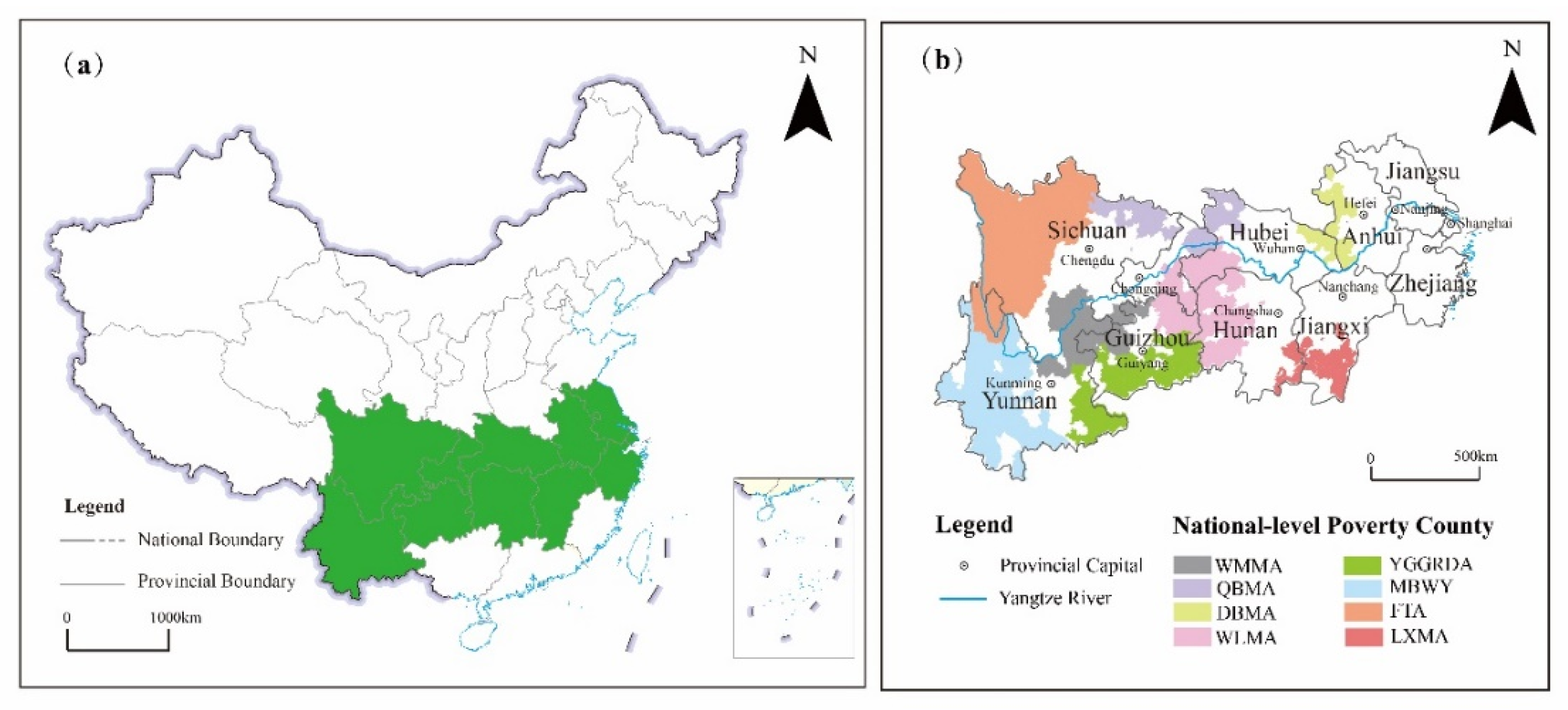
As one of the most strategically supporting regions in China, the Yangtze River Economic Belt (YREB) spans the three major regions of the east, central and west. It contains 1084 counties as well as many important urban aggregations (e.g., The Yangtze River Delta, the triangle of central China, and the Chengdu–Chongqing city group). Affected by differences in development conditions, poverty-stricken areas still exist in the YREB, such as the four Tibetan-inhabited areas and the Yunnan–Guizhou–Guangxi rocky desertification area. According to Chinese government statistics in 2015, there are still 346 national-level poverty counties in the YREB.
Figure 1 shows the geographical location of the YREB and the national-level poverty counties in this area. Given the adequacy of model training samples available in the YREB, the YREB is used as the study area of this paper. Moreover, there is also an evident contrast between the poverty samples and the wealth samples in this area. In addition, the county is the most basic administrative unit in China. The economic development condition and spatial distribution pattern of this unit is an intuitive manifestation of the current economic situation in the YREB [45]. Therefore, this paper selects counties as the basic study unit.
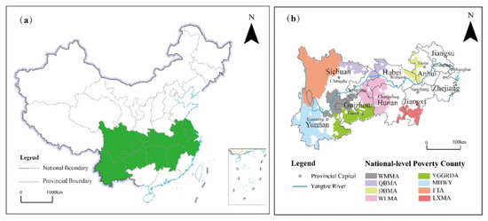
Figure 1.
Study area location: (a) Location of Yangtze River Economic Belt; (b) location of national-level poverty counties in Yangtze River Economic Belt. (Note: YREB represents the Yangtze River Economic Belt. FTA represents the four Tibetan-inhabited areas. MBWY represents the mountainous borderland of western Yunnan. QBMA represents the Qinba Mountain area. WLMA represents the Wuling Mountain area. WMMA represents the Wumeng Mountain area. YGGRDA represents the Yunnan–Guizhou–Guangxi rocky desertification area. DBMA represents the Dabie Mountain area. LXMA represents the Luoxiao Mountain area.).
2.2. Explanatory Variables
The 2030 Agenda determined that to eradicate poverty and achieve sustainable development, considering the three aspects of the economy, society and environment is necessary [1]. Therefore, this paper constructed a poverty explanatory variables table, which comprises three dimensions of natural, economic and social (Table 1). Based on this, the specific explanatory variables affecting poverty were chosen using an extensive literature review and expert knowledge. Several studies have also confirmed that the geographical (e.g., topographic, climatic and natural resources) and the socio-economic (e.g., economic, political and demographic) variables are indeed closely related to poverty [29,45,48,49,50,51]. The specific selection basis is as follows:

Table 1.
Multidimensional poverty explanatory variables.
In the natural dimension, considering that steep slopes, especially land with a slope higher than 15°, are unsuitable for use as farmland, the mean elevation and the proportion of land area with slopes higher than 15° were selected as explanatory variables to measure the natural terrain conditions of the county. The mean annual precipitation and cultivated land yield were selected because they can intuitively measure the regional water resource occupation and the productivity of cultivated land.
In the economic dimension, gross regional product (GRP) can characterize the risk of returning to poverty for residents in a region. The larger the value, the smaller the risk. In socio-economic variables such as per capita household savings, the proportion of secondary industry and per capita fiscal expenditure can comprehensively reflect the level and potential of regional economic development. The night light index was selected to measure the attraction and diffusion capacity of the counties.
In the social dimension, considering the compulsory education security and basic medical security in the basic needs of poverty, the number of hospital beds per capita and the proportion of compulsory education were selected to represent the supply capacity of regional medical services and education resources. The number of welfare institution beds per capita was selected to measure the level of regional welfare house construction. The proportion of phone access was selected because it can represent the capacity of the county to collect and disseminate information, thus measuring the information degree of the county.
In the variable selection process, the variance inflation factor (VIF) was used to measure the multicollinearity of the explanatory variables. The calculation formula of VIF is as follows:
Ri is the negative correlation coefficient of the regression analysis between ith explanatory variable (in Table 1) and the remaining explanatory variable in Table 1 [52]. According to existing research [53], the VIF of each explanatory variable is less than 7.5, explaining that there is no redundant variable.
The coordinate data of the county government are the latitude and longitude of the location of each county government, which are obtained from the Baidu Map platform. Digital elevation model data, with a resolution of 90 m, were obtained from the US Geological Survey website (https://lta.cr.usgs.gov/HYDRO1K, accessed on 1 September 2020). Rainfall data were derived from the Chinese National Meteorological Data Center (http://data.cma.cn/, accessed on 1 September 2020). The night light data derived from the DMSP/OLS data were provided by the National Atmospheric and Oceanic Administration (http://ngdc.noaa.gov/eog/download.html, accessed on 20 October 2020). Census data derived from the China County Statistical Yearbooks (1999~2016) and the Provincial Statistical Yearbooks (1999~2016) were collected by the Chinese government.
3. Methods
3.1. Model Definition
Definition 1.
Spatial vector V and spatial distance dataset D. Spatial vector V was used to describe the spatial correlation between counties, which is calculated by SVNN. The calculation process is as follows:
First, to obtain the spatial distance dataset D, the x and y coordinates were used to calculate the spatial distance between the ith county pi and other counties in turn. The x and y coordinates of the county pi are obtained from the latitude and longitude of the location of the county government. Dataset D can be presented by the following:
In Equation (2), dn,m represents the spatial distance between the nth county and the mth county. D is a symmetric matrix with a diagonal of 0, while the calculation method of spatial distance adopts the Euclidean distance. The equation is as follows:
In Equation (3), xn and yn are the longitude and latitude of the location of the nth county government. Therefore, the calculation of the space vector can be regarded as learning the SVNN model with the space distance dataset D as the input data. It can be expressed by Equation (4):
In Equation (4), Vn = {Vn,1,Vn,2, …Vn,6}, Vn is the spatial vector of the nth county. Because the number of SVNN output layer units was six, there are six elements in Vn.
Definition 2.
Explanatory variables dataset PN×M. P is an important part of the DNN input dataset, which is constructed by the county explanatory variables in Table 1, which can be expressed as P∈RN×M. Among them, N represents the county (N = 1084) and M represents explanatory variables (M = 15). The detailed input dataset P is shown in Equation (5):
In Equation (5), pn,m in P represents the characteristic value of the mth explanatory variable in the nth county. pn,1, pn,2, …, pn, and15 represents the characteristic values of the explanatory variables in Table 1. Therefore, the calculation of MPI can be expressed by Equation (6):
Definition 3.
Training sample. To obtain continuous MPI, the MPI output of the SVDNN model was set as a binary classification problem. The training sample contains two types of samples, namely the poverty sample and the wealth sample. The selection of the poverty sample was based on the national-level poverty counties designated by the Chinese government, and the sample value is set to 1. The selection of the wealth sample was based on the central cites of the Yangtze River Delta, and the sample value is set to 0. The closer MPI is to 1, the higher the poverty would be.
3.2. Model Structure
While commonly used machine learning models such as the random forest (RF) are widely used in the research of poverty probability classification and prediction research [44,45,46], the models above can only output discrete classification results, which may appear less capable of outputting continuous index results.
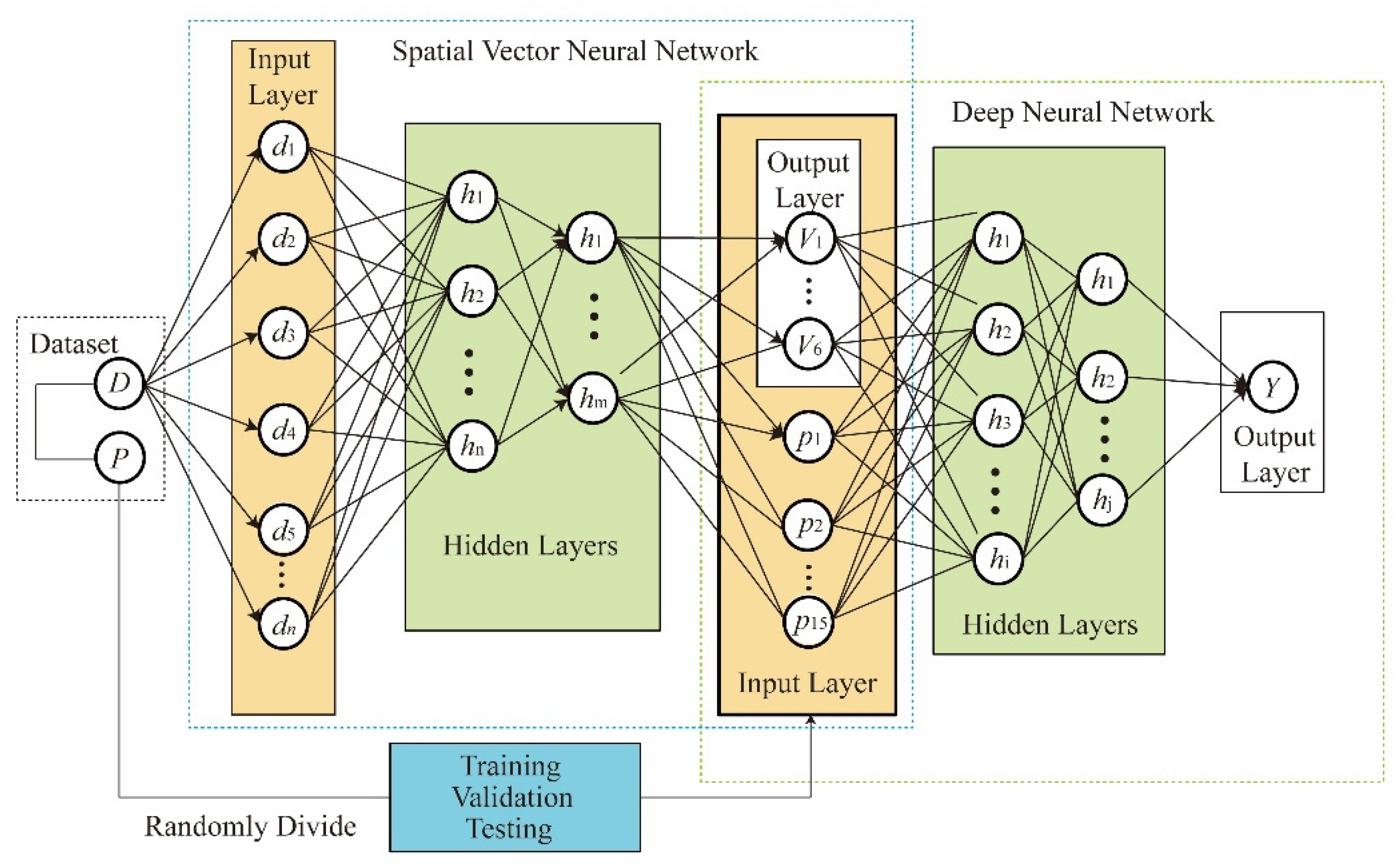
This paper overcomes this problem through the SVDNN model, whereby a specific output activation function sigmoid was used to map the MPI to the contiguous interval [0, 1]. First, the structure of SVDNN is shown in Figure 2. As Figure 2 has shown, the dataset P was randomly divided into a training set, a test set, and a validation set. Then, the SVNN calculated the spatial vector of the county. Finally, the spatial vector and explanatory variables were aggregated through the contact function provided by Tensorflow to calculate MPI by DNN. The Y output by the output layer is MPI. For the detailed algorithm design of SVNN and DNN, see Section 3.2.1 and Section 3.2.2.
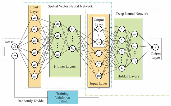
Figure 2.
Structure of SVDNN model.
3.2.1. SVNN
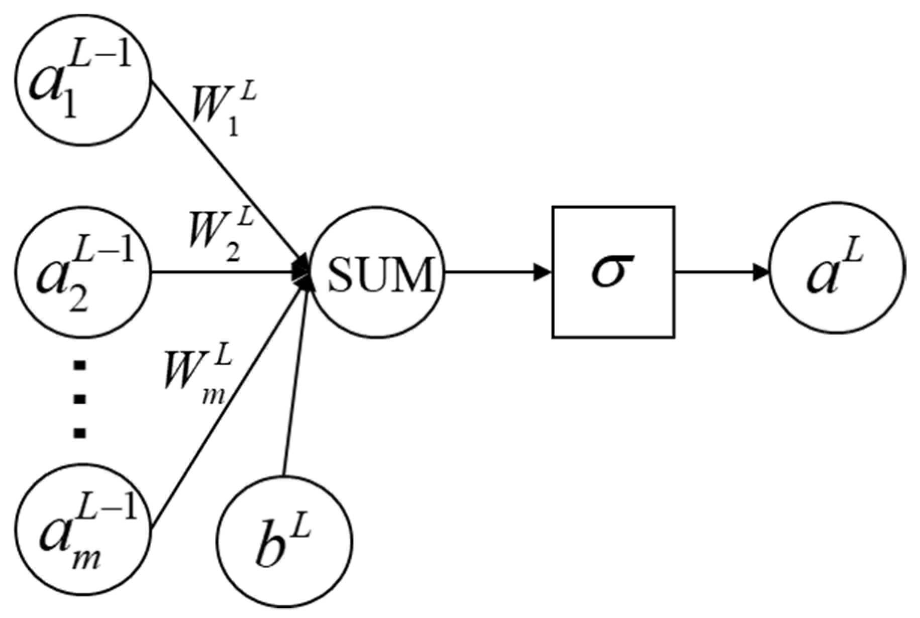
In the SVDNN model, the SVNN model uses error forward propagation. Figure 3 shows the transmission process of a single neuron in the SVNN model. In Figure 3, is the input data of the mth neuron in the L − 1 layer, is the weight, is the bias term, SUM is the summation function, is the activation function and is the output value of the output layer L.
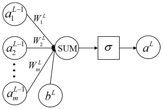
Figure 3.
The structure of SVNN single neuron.
The process above can also be expressed by Equation (7):
3.2.2. DNN
DNN was chosen to construct SVDNN because of its strong characterization ability, which can learn multidimensional and nonlinear features by stacking fully connected networks and nonlinear activation networks. It has been widely used in the modeling of spatio-temporal relationships [54,55].
In SVDNN, DNN was based on a multi-layer fully connected network and used an error back propagation to constrain network parameters to output results. A parameter update process is shown as follows:
In Equation (8), is the loss function. This paper uses binary cross entropy as the loss function, which is more suitable for a binary classification neural network with one output layer unit.
Take the derivative of Equation (8):
In Equation (9), is the output vector of the output layer L, is the output vector of the hidden layer l (l = 2, …, L − 1) and is the gradient vector of . The gradient vector of the hidden layer is further deduced from , where is defined as:
In Equation (10), can be replaced by the following Equation (11):
The relationship between and can be given by:
Substitute Equations (11) and (12) into Equation (10):
In Equation (13), represents the Hadamard product. After calculating , update the parameters of each network layer, for which the formula is as follows:
In Equation (14), is gradient vector and is the gradient element of the ith neuron on the hidden layer L. m is the total number of neuron in hidden layer l. is the weight vector of hidden layer L. is the bias term of the hidden layer L. is the learning rate. and are the weight vector and the bias term of the hidden layer l updated after the first iteration.
3.3. Model Evaluation Metrics
Because the output of the SVDNN model are continuous MPIs rather than discrete classification results, evaluation metrics such as the accuracy, recall and f1 score were not used in this paper. The four evaluation metrics were used to evaluate the model performance:
- Root mean square error (RMSE);
- 2.
- Mean absolute error (MAE);
- 3.
- Explained variance score (var)
- 4.
- Coefficient of determination (R2).
In Equations (15)–(18), N is the sample size, and and are the sample value and model prediction value. and are the dataset of sample value and model prediction value. is the mean value of and Var is the variance. The smaller the RMSE and MAE, the better the model performance will be. The maximum value of var and R2 is 1, and the closer to 1, the better the model performance will be.
3.4. Model Parameters Selection
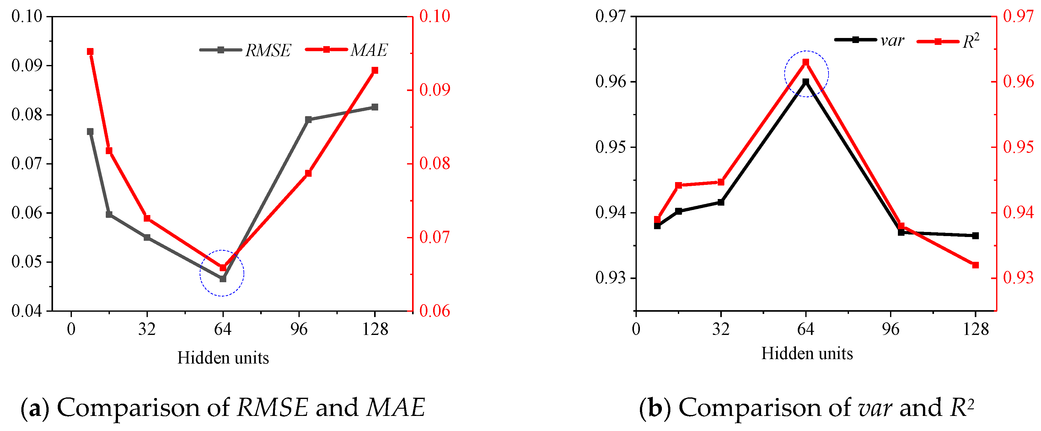
Selecting optimal model parameters (i.e., epoch, hidden units) is of paramount importance for neural network model training because the number of parameters with different numbers may greatly affect the accuracy of the model [56].
To determine the optimal number of epochs and hidden units, various numbers of epochs and hidden units were used for experimentation, and various evaluation metrics were used for determination, such as RMSE, MAE, var and R2. Figure 4 shows that when the epoch is equal to 450, RMSE and MAE are the lowest, while var and R2 are the highest. The epoch of SVDNN was set to 450. The number of hidden units was determined after the epoch was determined, as shown in Figure 5, which indicated that when the hidden units are equal to 64, RMSE and MAE are the lowest, and var and R2 are the highest. The number of hidden units of SVDNN was set to 64.
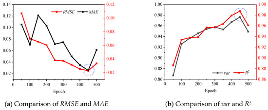
Figure 4.
Comparison of model performance under different epochs.

Figure 5.
Comparison of model performance under different epochs.
Combining Figure 4 and Figure 5, it can be found that with the increase in epoch and hidden units, RMSE and MAE first decrease and then increase, while var and R2 are the opposite, indicating that the model performance also increases first and then decreases. This variation may be caused by the over-fitting phenomenon in the training process.
For the input layer, the training dataset (60% of the total dataset) was used as the input in the training process, while the remaining data were used as the test dataset (20% of the total dataset) and the validation dataset (20% of the total dataset). To improve the computational performance of the model, several training parameters were also used in the training process, such as the Adam optimization, batch normalization [57] and dropout [58]. The sigmoid function was selected as the activation function of the output layer, which can continuously map the output value to [0, 1], and the output value can be directly used as MPI.
4. Results
4.1. Model Performance Comparison
The SVDNN model performance was compared with the following baseline models:
- Artificial Neural Network (ANN) [59]: ANN’s network layers adopted an error forward propagation, and the layers are fully connected;
- Back Propagation Neural Network (BPNN) [49]: A neural network trained according to an error back propagation. The basic idea of error back propagation is gradient descent;
- Deep Neural Network (DNN) [40]: DNN works in a similar way to ANN. The difference between DNN and ANN is that DNN has more hidden layers between the input layer and the output layer, which increased the computing capability of the model [60].
4.1.1. Comparison of the Spatial Correlation Structure
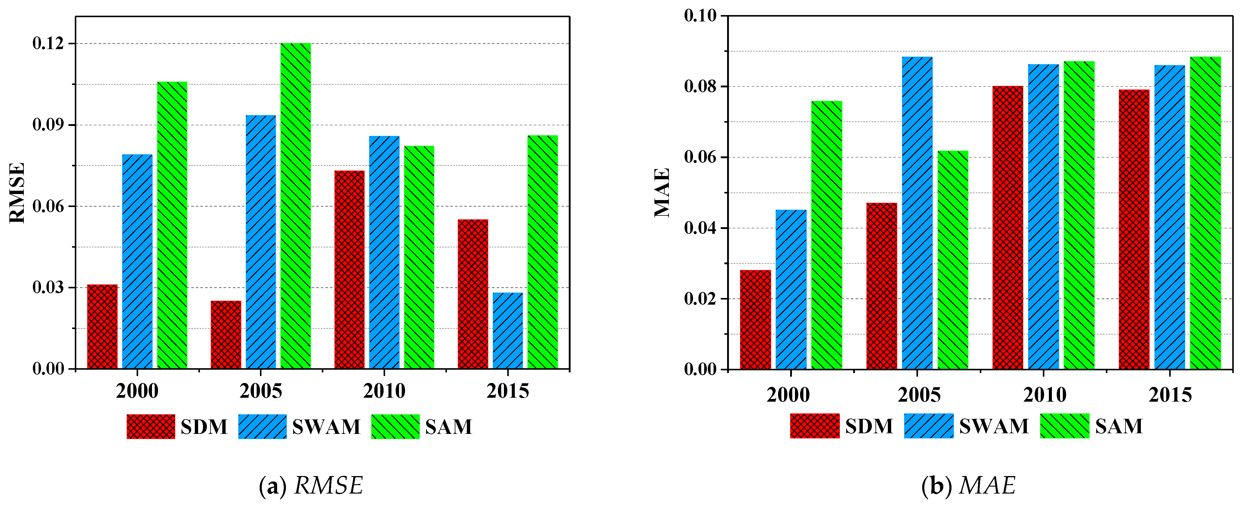
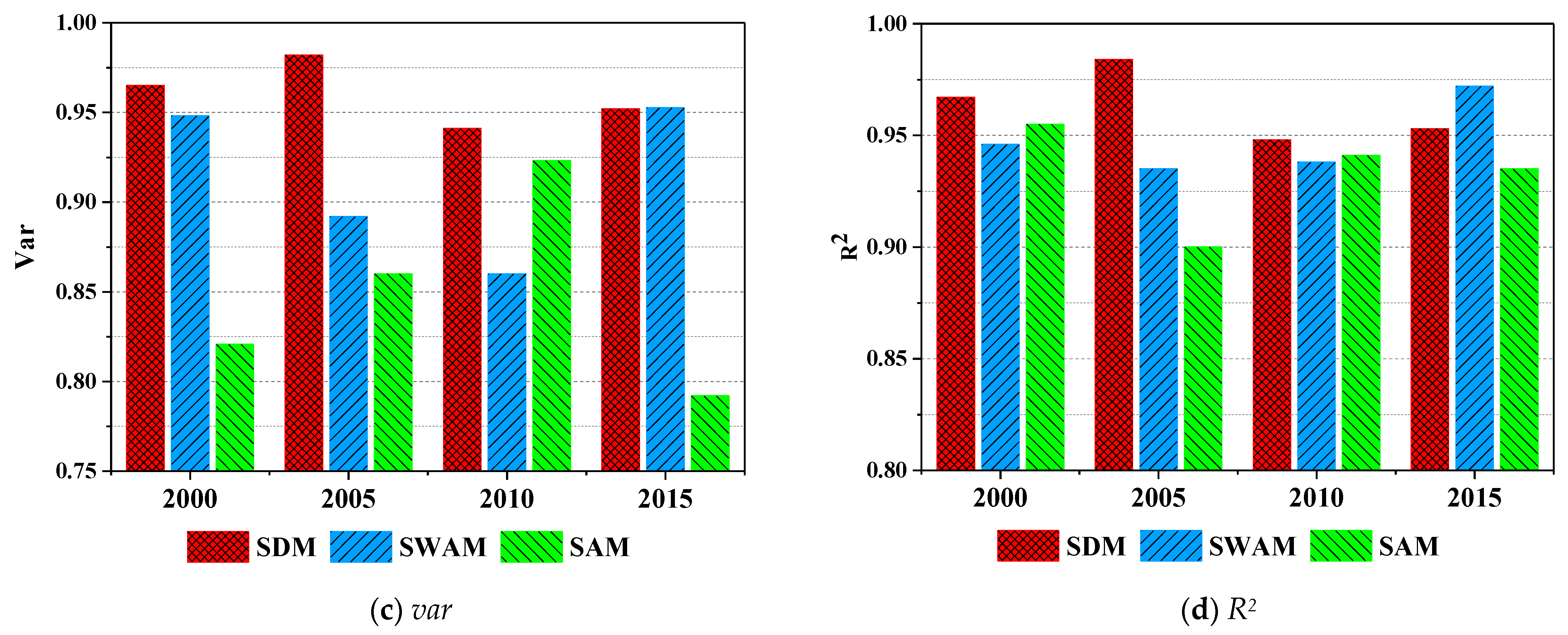
Spatial correlation structure is a critical input to the SVDNN model. However, the expression of spatial correlation structure is diverse, such as the spatial distance, topological relationship, etc. To determine the optimal spatial correlation structure, three types of structures were selected for experiments, and their evaluation metrics were calculated. The three structures were spatial distance matrix (SDM), spatial adjacency matrix (the adjacent area value was set to 1, while the non-adjacent area was set to 0) (SAM) and spatial weighted adjacency matrix (the matrix value of the adjacent area was the spatial distance, while the non-adjacent area was 0) (SWAM).
Figure 6 shows the evaluation metrics of the three spatial correlation structures. In 2000, 2005 and 2010, SDM had the best performance (RMSE and MAE were the lowest; var and R2 were the highest). Overall, the comprehensive model of SDM performed the best, followed by SWAM, while SAM was the worst.

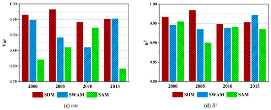
Figure 6.
Comparison of model performance under different spatial correlation structures. (Note: SDM represents the spatial distance matrix; SAM represents the spatial adjacency matrix (adjacent area value is set to 1, while the non-adjacent area is set to 0); SWAM represents the spatial weighted adjacency matrix (The matrix value of the adjacent area is the spatial distance, while the non-adjacent area is 0).
4.1.2. Comparison of the Evaluation Metrics
Table 2 shows the performance of the SVDNN model and other baseline models in calculating MPI in 2000, 2005, 2010 and 2015.
Table 2.
Evaluation metrics results of models.
As shown in Table 2, the values of RMSE and MAE of each model did not exceed 2, which were kept in a small numerical range. It is possible that the sample value of the poverty county was set to 1 and the wealth sample value was set to 0. In Table 2, the SVDNN model achieved the best performance in every year, which shows that the SVDNN model has the ability to capture spatial correlation between counties. Such an ability can be emphatically reflected in the model comparison between the SVDNN and the DNN because the difference between SVDNN and DNN is that the SVDNN model conducts the SVNN model before conducting the DNN model. Compared with DNN, the SVDNN’s RMSE decreased by 8.2%, while the R2 increased by 10.9% in 2015 (Table 2).
4.1.3. Comparison of the National-Level Poverty County
To validate whether the SVDNN model directly improves poverty identification accuracy, Figure 6 displays the poverty identification results for different models and compares them with the national-level poverty counties designated by the Chinese government.
As shown in Figure 6, the following can be observed: In the SVDNN identification results (Figure 7a), 252 poverty counties were correctly identified, with an accuracy of 72.83%, and unidentified counties and misidentified counties accounted for 10.87% and 16.30%. In the DNN identification results (Figure 7b), 204 poverty counties were correctly identified, with an accuracy of 58.96%, and unidentified counties and misidentified counties accounted for 11.90% and 29.14%. In the BPNN identification results (Figure 7c), 186 poverty counties were correctly identified, with an accuracy of 53.76%, while unidentified counties and misidentified counties accounted for 19.30% and 26.94%. In the ANN identification results (Figure 7d), 130 poverty counties were correctly identified, with an accuracy of 37.57%, while unidentified counties and misidentified counties accounted for 44.80% and 17.63%.
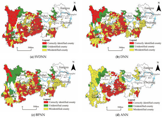
Figure 7.
Comparison of MPI identification results with national-level poverty counties. (Note: The identification rules for correctly identified counties, misidentified counties, and unidentified counties are as follows: First, the MPIs calculated by each model are divided into five values (low, mid-low, mid, mid-high and high) using the natural breaks classification. Second, the low value and mid-low value counties of the MPIs are divided into the poverty counties identified by the model and are examined to determine whether they belong to the national-level poverty counties. If they belong, the counties are identified correctly, if not, the counties are misidentified. Finally, the redundant poverty counties identified by the model or the counties belonging to the national-level poverty counties but not identified are divided into unidentified counties.).
The comparative analysis with the national-level poverty counties shows that the SVDNN model has a better identification accuracy compared with other baseline models. This indicates that the SVDNN model would obtain more accurate poverty information from the spatial distance dataset between the counties and the explanatory variable dataset than from measures based on the explanatory variable dataset.
4.1.4. Comparison of the Poverty Incidence
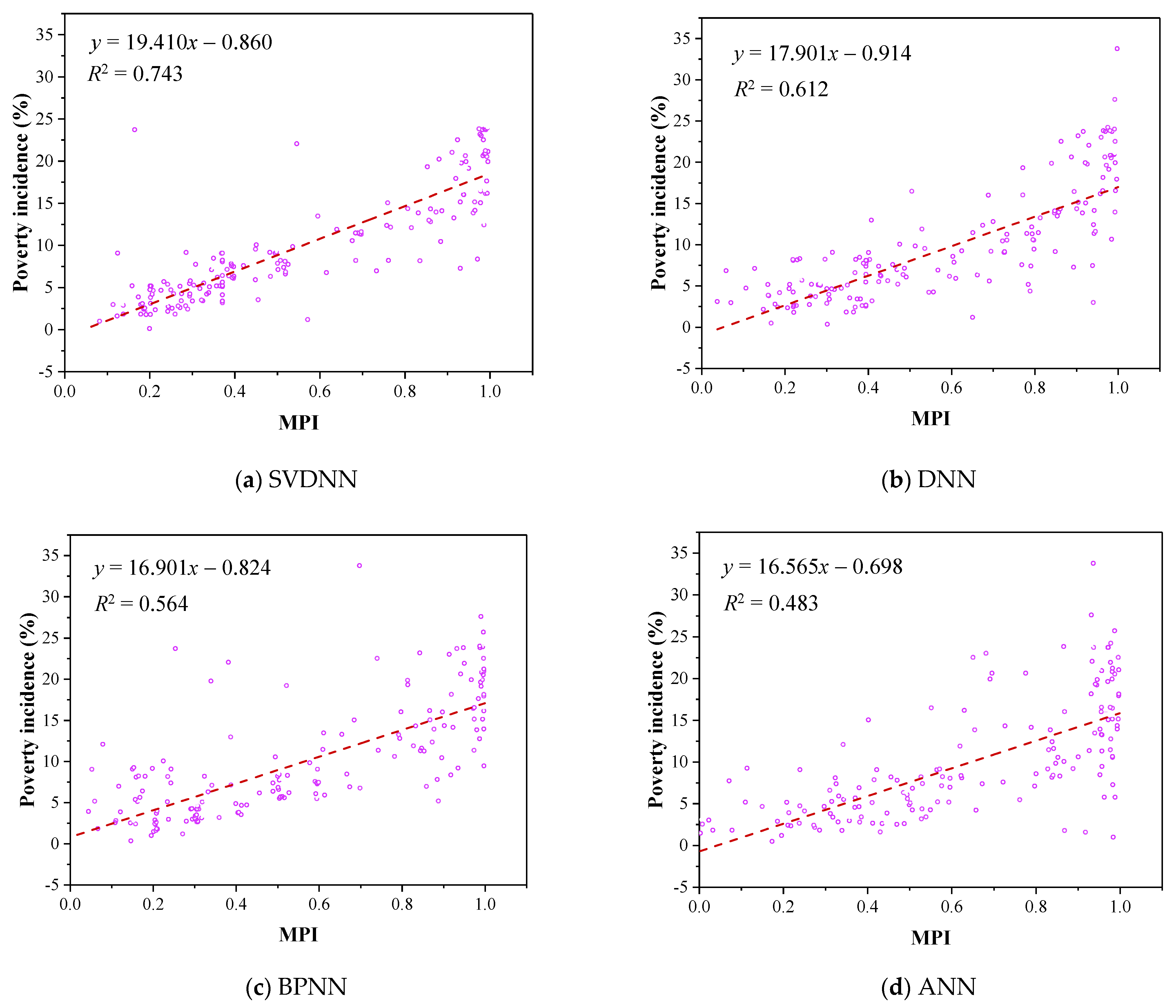
Given the strong correlation between MPI and poverty incidence, a linear regression was used to fit the MPI and the poverty incidence, based on the statistics of the county-level poverty incidence in 2015.
As seen Figure 8, the SVDNN model had the highest goodness of fit (R2 = 0.743), while the ANN model had the lowest goodness of fit (R2 = 0.483). In addition, SVDNN had the highest slope (19.410) and the highest concentration of scattered points, while ANN was the opposite, which indicated that the MPI results of the SVDNN model may have evident differences and regularity.
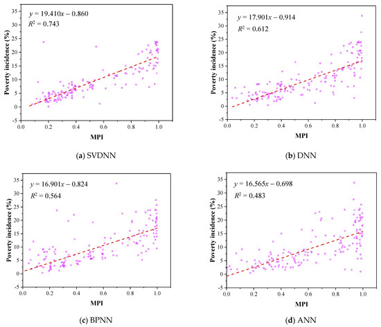
Figure 8.
Linear regression of MPIs and poverty incidence. (Note: Each scattered point represents a county, the abscissa is the MPI calculated by every model, and the ordinate is the poverty incidence rate corresponding to this county obtained from the county-level census data released by the Chinese government.)
4.2. Distribution Characteristics of MPI
4.2.1. Statistical Distribution Characteristics
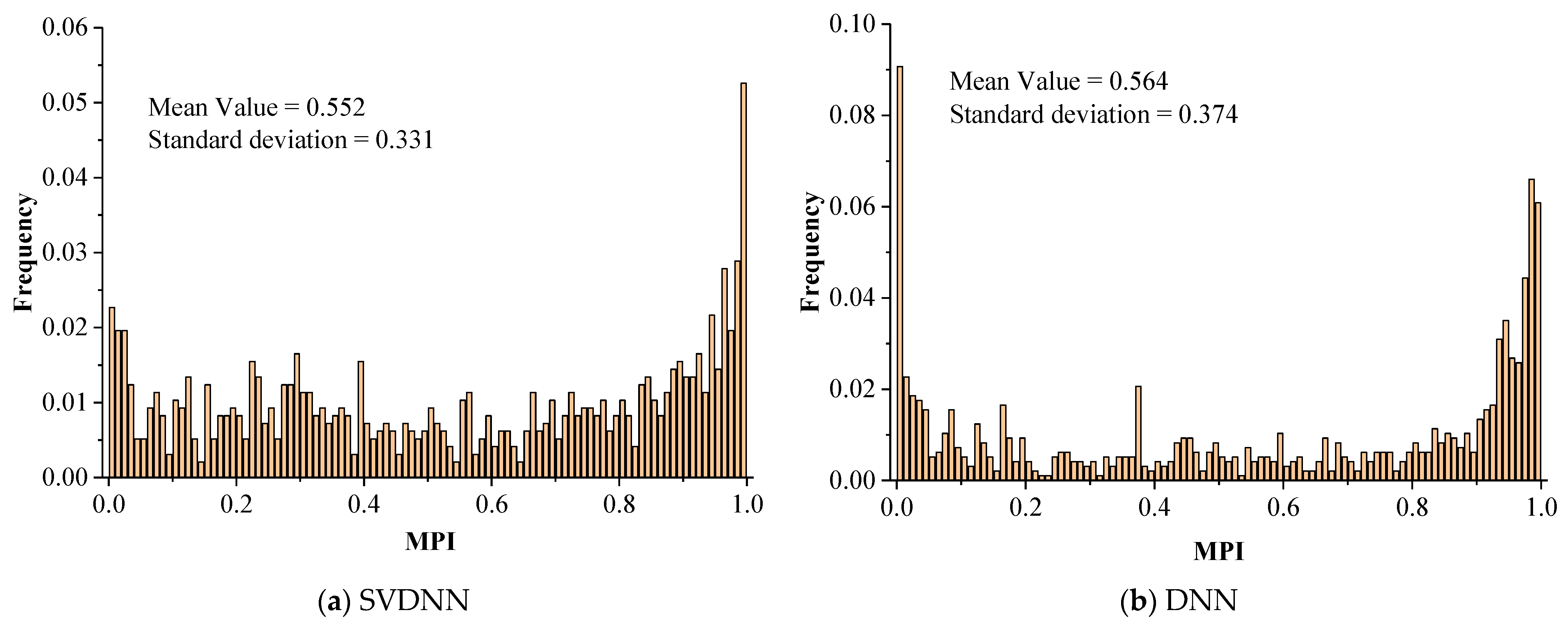
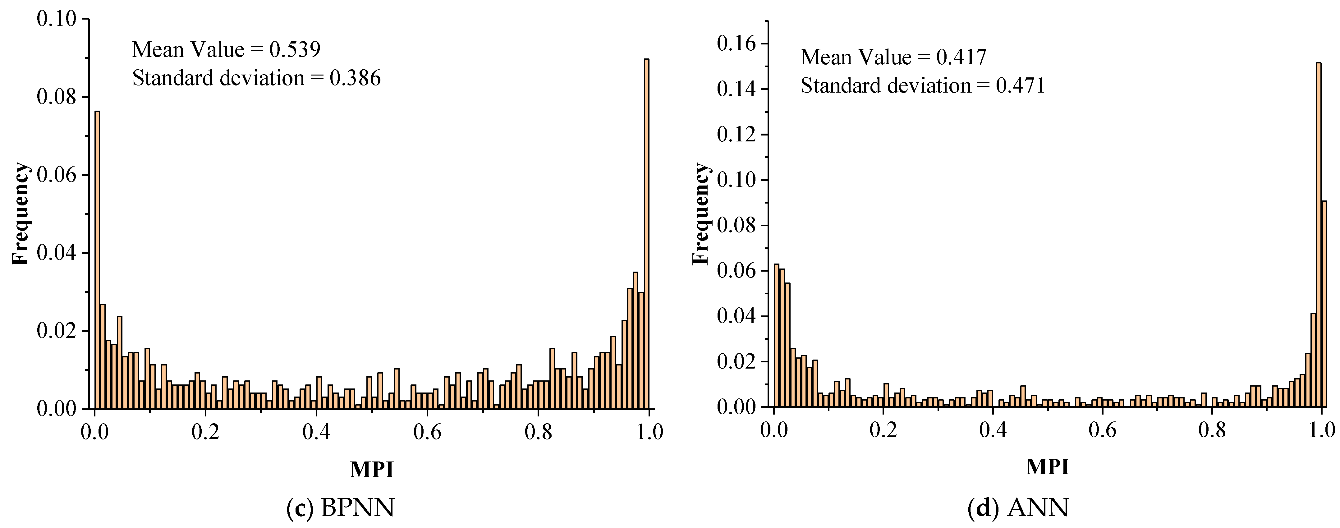
The frequency histograms of the 2015 MPIs calculated by the SVDNN model and other baseline models are shown in Figure 9. It used the mean value and standard deviation to measure the degree of concentration and dispersion of MPIs. The smaller the standard deviation, the less the MPIs deviated from the mean value and vice versa. Low standard deviation indicates that the MPI result and the corresponding calculated model may have a highly stable performance for the MPI in a different county.
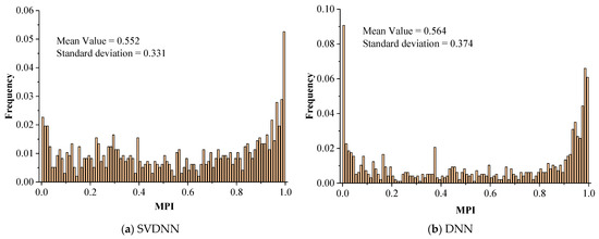
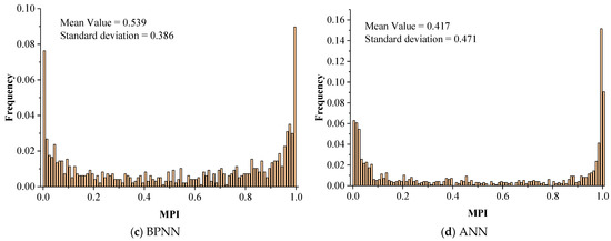
Figure 9.
Frequency distribution histogram of MPIs.
As shown in Figure 8, MPIs calculated by four models performed similarly, with the distribution characteristics of “low in the middle and high at both sides”. A possible explanation for this is that the SVDNN model and other baseline models chose the same training parameters. The mean values of SVDNN, DNN, BPNN and ANN were decreased (0.552, 0.548, 0.539 and 0.417), while the standard deviations were increased (0.331, 0.374, 0.386 and 0.471). Compared with other baseline models the frequency of the MPIs distribution of SVDNN was the highest in the (0.2, 0.8) interval. These results indicate that the SVDNN model had a better stability performance and is thus a more suitable method for calculating MPIs.
4.2.2. Spatio-Temporal Distribution Characteristics
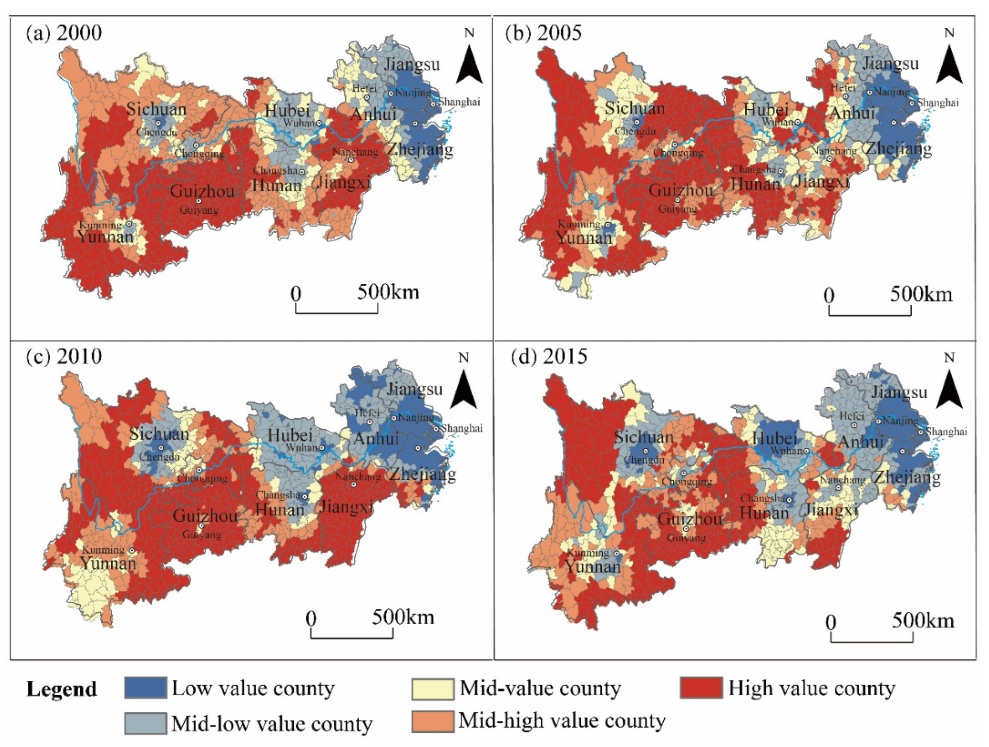
The calculated MPIs were continuous indices, but for an intuitive display, this paper divides them into five levels (Figure 10). Figure 10 illustrates the following: From the spatial scale, the MPIs present the spatial differentiation characteristics of “the central city is low and the city periphery is high”. The Yangtze River Delta, the triangle of central China, and the Chengdu–Chongqing city group were low-value agglomeration areas of MPI, and the degree of agglomeration decreased with the scale of the urban agglomeration from east to west, whereas the high-value areas of MPI were mainly concentrated in remote mountainous areas, border areas and ethnic minority areas in the central and western regions, such as the YGGRDA and the FTA.
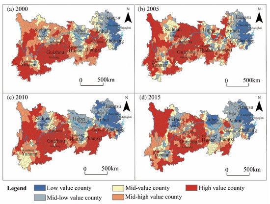
Figure 10.
Spatio-temporal distribution of MPIs. (Note: The MPI of each county is divided into five levels according to the natural breaks classification, which are high-value counties (1.000 ≥ MPI > 0.883), mid-high value counties (0.883 ≥ MPI > 0.686), mid-value counties (0.686 ≥ MPI > 0.437), mid-low value county (0.437 ≥ MPI > 0.167) and low-value counties (0.167 ≥ MPI > 0.000)).
From the time scale, the mean values of MPI in 2000, 2005, 2010 and 2015 were 0.741, 0.672, 0.667 and 0.552. The multidimensional poverty of the YREB has declined over time. From 2000 to 2010, the spatial agglomeration of high-value counties and low-value counties gradually increased. The counties with evident changes in MPI are mainly located in the middle reaches of the Wuhan metropolitan area and Changsha as well as theirs surrounding counties. The MPIs of the counties above both decreased, while the low-value counties spread to northern Hunan and eastern Hubei. The spatial characteristics of the low-value and mid-value areas have evolved from the sporadic distribution in 2005 to agglomerations in 2010, thus showing a trend of extending to the Yangtze River Delta. Compared with the previous period, the number of high-value counties in the YREB no longer dominated in 2015, whereas 17.81% of high-value counties have been reduced, and the number of low-value counties has increased from 15.83% to 20.10%.
4.3. Relative Contributions of Explanatory Variables to MPI
Also due to the fact that different models have different performances, various explanatory variables cannot make equal contributions to multidimensional poverty [61]. Such contributions can be quantitatively measured by the neural network connection weights of explanatory variables. These contributions provide a reference for the explanatory variable selection of other poverty measurement studies. The contributions of explanatory variables to MPIs were determined through calculating the mean value of relative contributions of each explanatory variable under the four neural network models (Table 3).
Table 3.
Relative contributions of explanatory variables to MPI under different models.
In Table 3, the contribution of the same explanatory variable in different models was different. In the training process using consistent training parameters, the differences in MPIs calculated by different models were mainly reflected in the weights assigned to the explanatory variables by a different model. For instance, in the DNN, BP and ANN models, the contribution of the mean elevation to MPI was 0.0673, 0.0681 and 0.0463, while in the SVDNN model, the contribution of average altitude to MPI was up to 0.1759. These differences are also partially driven by the calculation principles of different models that are different; for example, DNN used the error forward propagation, while BPNN used the error back propagation. In addition, the mean elevation, proportion of land area with a slope higher than 15°, per capital GRP and proportion of primary industry were the most important explanatory variables in the SVDNN, DNN, BPNN and ANN models.
Although the weights assigned to the explanatory variables by model were biased, from the mean value, the weight difference between explanatory variables does not exceed 0.064, indicating that the explanatory variables above have a certain contribution to MPIs. Therefore, the explanatory variables selected in this paper can be used as a powerful reference for poverty measurement research.
5. Discussion
5.1. Poverty Measurement and Identification
The inaccuracy of poverty measurement methods is hampering the efforts to identify regional poverty differences and effectively intervene in areas of the greatest poverty alleviation need, which places great pressure on poverty alleviation work [6,7,8,39]. Consequently, improving the identification accuracy of poverty measurement methods is of great significance to policy makers and researchers. The recent application of machine learning methods has led to a marked improvement in poverty measurement accuracy [44,45,46], but these methods only reflect the spatial correlation between poverty areas in the selection of explanatory variables or the visualized analysis of the poverty identification results. These techniques neglect the spatial correlation between the near and far areas in the calculation process of the poverty measurement.
However, spatial correlation, as an important reference for describing and understanding the socio-economic phenomenon of poverty, is also essential for poverty measurement. Thus, the key issue to improving the accuracy of poverty area identification is incorporating the spatial correlation between areas into the calculation process of poverty measurement. The design idea of the SVDNN model is similar to the basic concept of “We can better understand a person according to his/her friends” mentioned by Liu [62]. The SVDNN model first vectors the spatial distance between the counties and calculates the MPIs based on the explanatory variable dataset. The MPIs calculated by this model were closer to the real poverty situation.
To determine the optimal model expression structure of SVDNN, this paper quantitatively measured the model performance of SDM, SWAM and SAM through evaluation metrics. Then, the best model parameters were determined by assigning the epoch and hidden units different values. The model performance of SDM, SWAM and SAM decreased (see Section 4.1.1). The performance of SWAM was superior to SDM, showing that it insufficiently expresses the spatial correlation by relying on the topological relationship between two regions. Taking the spatial distance as the weight of the adjacency matrix can further simulate and quantify the spatial correlation between regions. From the comparison of SDM and SWAM, it is more appropriate to use a SDM than SWAM. The difference in model performance can be attributed to SWAM, which only measures the effect of adjacent areas. However, all areas around an area have corresponding radiation effects or siphon effects on the area, and the closer the distance, the stronger the effect. SDM is substantially superior in quantitatively measuring spatial correlation than the other two structures.
To demonstrate the model performance of the SVDNN, three baseline models of the DNN, BPNN and ANN in related poverty research were selected for comparison [40,49,59]. Commonly used machine learning methods such as RF and SVM were not used for comparison because although the machine learning methods above have shown promise in computing discrete poverty classification results, they appear less capable of outputting continuous index results in binary classification problems, while the MPIs calculated in this paper were continuous indices, which can reflect the changing trends of each county.
The MPIs calculated by the SVDNN model and other baseline models were compared in respect to three metrics: the evaluation metrics, the national-level poverty counties and the poverty incidence. The comparison results were consistent. The error back propagation mechanism of BPNN made its performance better than that of ANN. The DNN model with multiple hidden layers had a better identification accuracy than BPNN, indicating that the deep network structure can improve the learning ability of the model [57,60]. Therefore, in the construction of the SVDNN model an error back propagation mechanism and a deep network structure were used. To avoid the over-fitting phenomenon in the training process, the optimal parameters were also determined through experiments.
In addition, because each model adopts a fully connected method, each explanatory variable has a corresponding connection weight. The contribution of each explanatory variable in different models was derived from the mean value of the connection weight. The SVDNN has the highest identification accuracy, in which the weight of explanatory variables in the SVDNN model is of paramount importance. In this model, the explanatory variable with the highest contribution was the mean elevation, which indicates that the SVDNN model regards geographical environment variables as the determinant of poverty after vectorizing the spatial correlation between counties. This result also illustrates the rationality of the SVDNN model for weighing explanatory variables because existing studies indicate that the mean elevation has a spatial neighbor-based correlation with poverty incidence [63], which is also the fundamental control factor explaining the spatial pattern of poverty [29].
The proportion of secondary industry, per capita fiscal expenditure, number of welfare institution beds per capita and proportion of land area with a slope higher than 15° would be reliable explanatory variables for poverty measurement.
Finally, models for calculating MPIs in all counties in the YREB performed similarly, with the slope and intercept of the regression equation of each model exhibiting small differences (see Section 4.1.3), and the MPIs calculated by each model showed similar frequency distribution characteristics (see Section 4.2.1). The discussion above illustrates the robustness and applicability of the neural network model in poverty measurement. However, the SVDNN, which incorporates spatial correlation into the calculation process, can provide a better performance in measuring MPIs than other baseline models. This demonstrates that the SVDNN would obtain more accurate information estimates based on the spatial distance dataset and explanatory variables dataset than other baseline model estimates based on the explanatory variable dataset only.
5.2. Spatio-Temporal Characteristics of MPI
The MPIs formed a spatial pattern with the Yangtze River Delta as the low-value agglomeration center, while Wuhan, Changsha, Chengdu and other central cities constitute the low-value sub agglomeration center. Such characteristics were highly similar to the evolution of urban agglomeration [64]. From 2000 to 2015, the number of high-value poverty counties decreased over time, and its decrease in spatial range was centered in the provincial capital cities in the middle and upper reaches of the Yangtze River and extended to the periphery of the city. This evolution is consistent with the economic radiation generated by the provincial capital cities.
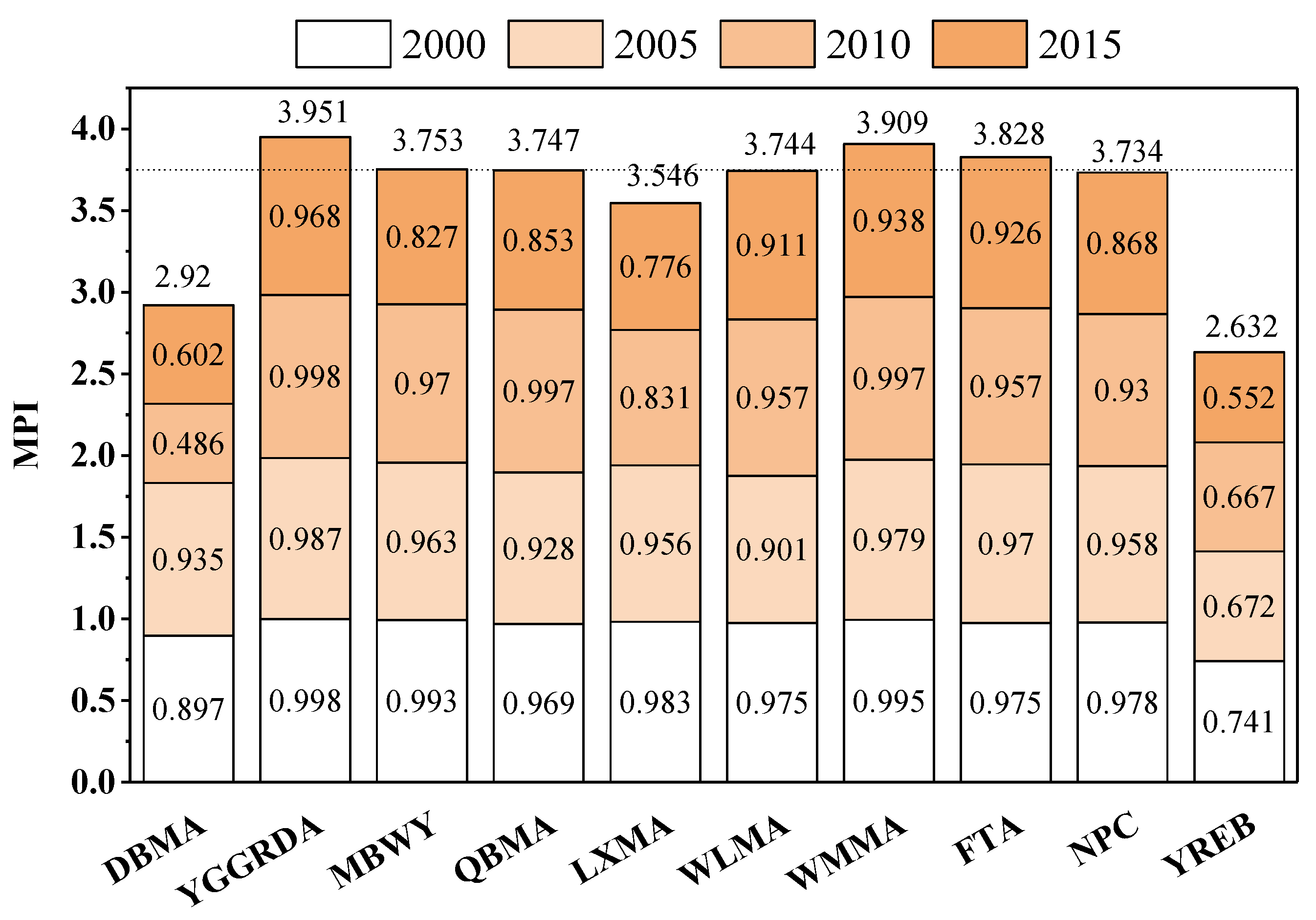
Compared with the counties surrounding the urban agglomerations where the poverty condition is easily improved, the MPIs of the national-level poverty counties are shown in Figure 11. As shown in Figure 11, the mean MPIs of the DBMA and the LXMA were lower than the mean MPIs of the national-level poverty counties. The mean MPIs of the YGGRDA, the WMMA and the FTA were relatively high, and they have been in a deep multidimensional poverty state for a long time. These findings are understandable because they are consistent with the poverty alleviation effect brought by the geographical location of national-level poverty counties. For example, the MPI of the DBMA and the LXMA was lower because the aforementioned areas have superior social, economic and natural environments compared with the inland areas [34]. Their advantageous socio-economic and natural environment basic conditions compared with the inland poverty counties mainly drives the lower MPIs of the DBMA and the LXMA [55], whereas the YGGRDA, the WMMA and the FTA belong to the rocky desertification areas in southwestern China, with high altitudes, steep slope and low resource capacities, which are inconducive to the work of poverty alleviation [48,63].
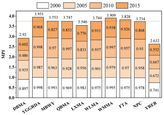
Figure 11.
MPIs of national-level poverty counties. (Note: YREB represents the Yangtze River Economic Belt. FTA represents the four Tibetan-inhabited areas. MBWY represents the mountainous borderland of western Yunnan. QBMA represents the Qinba Mountain area. WLMA represents the Wuling Mountain area. WMMA represents the Wumeng Mountain area. YGGRDA represents the Yunnan–Guizhou–Guangxi rocky desertification area. DBMA represents the Dabie Mountain area. LXMA represents the Luoxiao Mountain area. NPC represents the national-level poverty counties.).
5.3. Applicability of SVDNN Model
The SVDNN model demonstrates the applicability of the research area and object. The first is the applicability of the research area. The UN 2030 Agenda proposed that the goal of eradicating poverty is still the primary factor in achieving Sustainable Development Goals all over the world. Therefore, discussing the applicability of this model in different regions and even different countries is necessary.
Whether it is an advanced economy or an emerging country, an area’s socio-economic development level can be divided into three levels: poverty (low and mid-low value county), median (mid value county) and wealth (high and mid-high value county). For the identification of poverty areas, SVDNN has shown a better model performance than other baseline models (see Section 4.1.3). For the median area, the frequency distribution of MPI calculated by the traditional neural network method is obviously extreme (see Section 4.2.1). For example, the ANN only identified 7.84% of the mid-value counties, but the true proportion of the mid-value counties (non-national poverty county and non-urban agglomeration) in the YREB was 17.42%. However, SVDNN successfully identified 20.20% of the mid-value counties, which is the highest percentage identified among the three baseline models and most consistent with the real situation, indicating that SVDNN is most sensitive to the multidimensional poverty in the median area. For the wealth areas, the true proportion of urban agglomerations in the YREB is 37.73. The SVDNN identification results accounted for 41.03%, while those of ANN accounted for as high as 45.8%. Thus, the identification accuracy of the SVDNN model is better than that of the traditional neural network model, which shows the applicability of the SVDNN model in various regions and countries.
The second is the applicability of the research object. From Figure 6 and Table 2, the model performance of SVDNN, which incorporates spatial correlation structures (SDM, SWAM, SAM), was better than that of other baseline models, indicating that spatial correlation is a critical input to poverty measurement. However, poverty is not the only phenomenon with spatial correlation; ecological vulnerability [65], transport accessibility [66], economic development level [67] and other research objects are also affected by the surrounding area. Therefore, even if the research object changes, the geographical index calculation studies of the SVDNN model could have a broad application across many geographical domains and may be immediately useful for producing measurement indices with higher precision than the traditional neural network.
5.4. Policy Application
Measuring poverty can importantly influence how we understand it and how we create policies to influence it [20]. According to the poverty measurement of YREB, the two policy applications can be proposed:
First, given the spatio-temporal characteristics of multidimensional poverty in the YREB, the wealth areas and the urban aggregation should play a leading role in strengthening the radiation power of regional central cities. Other counties should also strengthen their cooperation with neighboring high-value counties and gradually narrow the poverty gap between regions. Second, as the YGGRDA and WMMA have been in a state of deep multidimensional poverty for a long time, policy makers should pay more attention to the rocky desertification area in the southwest when formulating the next step of poverty alleviation policies. For the areas above, strengthening the construction of water storage and irrigation facilities is necessary to improve the efficiency of karst groundwater utilization.
5.5. Limitations
The accuracy of poverty measurement not only depends on the efficiency and effectiveness of the model but also on the selection of reliable poverty explanatory variables because the explanatory variables have been shown to correlate partly with the improvement of identification accuracy [6,41]. However, there is still no complete standard for the selection of poverty explanatory variables. This gap can be attributed to the different regions, which have different livelihoods and political strategies, as the poor nations are still lacking the budget and technology to collect census data [31,32]. Thus, future poverty measurement studies should be conducted to select a reasonable poverty explanatory variable system that also adapts to local conditions. In addition, this SVDNN method only considers spatial correlation, but does not consider temporal correlation. Future poverty research could also focus on the model construction of spatio-temporal correlations between poor regions.
6. Conclusions
This paper proposes a new multidimensional poverty measurement method, the SVDNN model, which incorporates spatial correlation between counties, and further compared the model performance of this model with the three baseline models of DNN, BPNN and ANN. The SVDNN model was used to calculate the MPIs of the YREB in 2000, 2005, 2010 and 2015. Finally, the contribution of different explanatory variables to MPIs was also calculated.
The main contribution of this paper is the proposal of a SVDNN model to identify poverty objects. The SVDNN quantitatively expresses spatial correlation between areas and incorporates it into the calculation of the poverty measurement. This model shows a superior model performance than traditional neural network models, which can effectively improve the accuracy of poverty object identification. Given the applicability of YREB’s poverty identification to data from 2000 to 2015, this model can also contribute to large-scale, dynamic and long-term poverty identification in advanced economics and emerging counties. The second contribution is revealing the importance of various influencing factors in multi-dimensional poverty, which can provide a reference for the selection of variables for the measurement of multi-dimensional poverty. Based on the analytical and experimental results presented in this paper, the following conclusions may be reached:
- In the four comparisons of the spatial correlation structure, evaluation metrics, national-level poverty counties and poverty incidence, the SDM exhibited a superior model performance than the SAM and SWAM and is more suitable for the construction of the SVDNN models. The SVDNN model, by incorporating the spatial correlation (SDM, SAM and SWAM) between areas, provided better poverty identification accuracy compared with the three baseline models of DNN, BPNN and ANN. However, the performance of the SVDNN model is optimal.
- The MPIs calculated by various neural network models performed similarly in the frequency distribution and the linear regression of poverty incidence. Such similarity reflected the robustness and applicability of the neural network model in poverty measurement.
- Urban agglomerations in the Yangtze River Delta, the Triangle of Central China, and Chengdu-Chongqing city group were low-value MPI agglomeration areas, and the degree of agglomeration decreased with the scale of urban agglomerations from east to west. The YGGRDA, the WMMA and the FTA have been in a state of deep multidimensional poverty for a long time. The spatio-temporal characteristics of MPI above were consistent with the influence of urban agglomeration and geographical location.
- In the SVDNN model, the mean elevation, proportion of secondary industry, per capita fiscal expenditure, number of welfare institution beds per capita and the proportion of land area with a slope higher than 15° have a higher contribution to MPIs, and they would be reliable explanatory variables for poverty measurement.
Author Contributions
Conceptualization, Qianqian Zhou and Nan Chen; methodology, Qianqian Zhou; software, Qianqian Zhou and Siwei Lin; validation, Qianqian Zhou; formal analysis, Qianqian Zhou; investigation, Nan Chen; resources, Qianqian Zhou, Siwei Lin and Nan Chen; data curation, Qianqian Zhou and Siwei Lin; writing—original draft preparation, Qianqian Zhou and Nan Chen; writing—review and editing, Qianqian Zhou and Nan Chen; visualization, Qianqian Zhou; supervision, Nan Chen; project administration, Qianqian Zhou and Nan Chen. All authors have read and agreed to the published version of the manuscript.
Funding
This research was funded by the National Natural Science Foundation of China (grant numbers 41771423).
Institutional Review Board Statement
Not applicable.
Informed Consent Statement
Not applicable.
Data Availability Statement
The vector boundary data of county were derived from the National Basic Geographic Information Center (http://www.ngcc.cn/ngcc/, accessed on 10 May 2020). The list of national-level poverty counties came from the National Natural Resources and Geospatial Basic Information Database (http://www.geodata.gov.cn/web/geo/index.html, accessed on 10 May 2020). The base map of the Yangtze River Economic Belt was obtained from the standard map service website of the National Bureau of Surveying and Mapping (http://bzdt.ch.mnr.gov.cn/, accessed on 10 May 2020).
Acknowledgments
We thank the editors and the anonymous reviewers for their valuable comments and suggestions.
Conflicts of Interest
The authors declare no conflict of interest.
References
- UN. Transforming Our World: The 2030 Agenda for Sustainable Development; UN: New York, NY, USA, 2015.
- Lynch, A.J.; Cowx, I.G.; Fluet-Chouinard, E.; Glaser, S.M.; Phang, S.C.; Beard, T.D.; Bower, S.D.; Brooks, J.L.; Bunnell, D.B.; Claussen, J.E.; et al. Inland fisheries—Invisible but integral to the UN Sustainable Development Agenda for ending poverty by 2030. Glob. Environ. Change 2017, 47, 167–173. [Google Scholar] [CrossRef]
- Mani, A.; Mullainathan, S.; Shafir, E.; Zhao, J. Poverty impedes cognitive function. Science 2013, 341, 976–980. [Google Scholar] [CrossRef] [PubMed] [Green Version]
- Haushofer, J.; Fehr, E. On the psychology of poverty. Science 2014, 344, 862–867. [Google Scholar] [CrossRef] [PubMed]
- Liu, Y.; Guo, Y.; Zhou, Y. Poverty alleviation in rural China: Policy changes, future challenges and policy implications. China Agric. Econ. Rev. 2018, 10, 241–259. [Google Scholar] [CrossRef] [Green Version]
- Jean, N.; Burke, M.; Xie, M.; Davis, W.M.; Lobell, D.B.; Ermon, S. Combining satellite imagery and machine learning to predict poverty. Science 2016, 353, 790–794. [Google Scholar] [CrossRef] [PubMed] [Green Version]
- Liu, Y.; Xu, Y. A geographic identification of multidimensional poverty in rural China under the framework of sustainable livelihoods analysis. Appl. Geogr. 2016, 73, 62–76. [Google Scholar] [CrossRef]
- Xu, Z.; Cai, Z.; Wu, S.; Huang, X.; Liu, J.; Sun, J.; Su, S.; Weng, M. Identifying the Geographic Indicators of Poverty Using Geographically Weighted Regression: A Case Study from Qiandongnan Miao and Dong Autonomous Prefecture, Guizhou, China. Soc. Indic. Res. 2018, 142, 947–970. [Google Scholar] [CrossRef]
- Deininger, K.; Squire, L. A new data set measuring income inequality. World Bank Econ. Rev. 1996, 10, 565–591. [Google Scholar] [CrossRef]
- Ravallion, M.; Chen, S. China’s (uneven) progress against poverty. J. Dev. Econ. 2007, 82, 1–42. [Google Scholar] [CrossRef] [Green Version]
- Brady, D. Rethinking the sociological measurement of poverty. Soc. Forces 2003, 81, 715–751. [Google Scholar] [CrossRef] [Green Version]
- Mohanty, S.K.; Agrawal, N.K.; Mahapatra, B.; Choudhury, D.; Tuladhar, S.; Holmgren, E.V. Multidimensional poverty and catastrophic health spending in the mountainous regions of Myanmar, Nepal and India. Int. J. Equity Health 2017, 16, 21. [Google Scholar] [CrossRef] [Green Version]
- Sen, A. Poverty: An ordinal approach to measurement. Econometrica 1976, 44, 219–231. [Google Scholar] [CrossRef]
- Lucchini, M.; Butti, C.; Assi, J.; Spini, D.; Bernardi, L. Multidimensional Deprivation in Contemporary Switzerland Across Social Groups and Time. Sociol. Res. Online 2014, 19, 42–55. [Google Scholar] [CrossRef] [Green Version]
- Wagle, U. Rethinking poverty: Definition and measurement. Int. Soc. Sci. J. 2002, 54, 155–165. [Google Scholar] [CrossRef]
- Park, A.; Wang, S.; Wu, G. Regional poverty targeting in China. J. Public Econ. 2002, 86, 123–153. [Google Scholar] [CrossRef]
- Alkire, S. Dimensions of human development. World Dev. 2002, 30, 181–205. [Google Scholar] [CrossRef]
- Alkire, S.; Santos, M.E. Measuring acute poverty in the developing world: Robustness and scope of the multidimensional poverty index. World Dev. 2014, 59, 251–274. [Google Scholar] [CrossRef] [Green Version]
- Arcagni, A.; Elisa, B.D.B.; Fattore, M.; Rimoldi, S.M.L. Multidimensional analysis of deprivation and fragility patterns of migrants in lombardy, using partially ordered sets and self-organizing maps. Soc. Indic Res. 2018, 141, 551–579. [Google Scholar] [CrossRef]
- Alkire, S.; Foster, J. Understandings and misunderstandings of multidimensional poverty measurement. J. Econ. Inequal. 2011, 9, 289–314. [Google Scholar] [CrossRef] [Green Version]
- Alkire, S.; Foster, J. Counting and multidimensional poverty measurement. J. Public Econ. 2011, 95, 476–487. [Google Scholar] [CrossRef] [Green Version]
- Foster, J.; Greer, J.; Thorbecke, E. The Foster-Greer-Thorbecke (FGT) poverty measures: 25 years later. J. Econ. Inequal. 2010, 8, 491–524. [Google Scholar] [CrossRef]
- Arndt, C.; Mahrt, K.; Hussain, M.A.; Tarp, F. A human rights-consistent approach to multidimensional welfare measurement applied to sub-Saharan Africa. World Dev. 2018, 108, 181–196. [Google Scholar] [CrossRef]
- Bennett, C.J.; Mitra, S. Multidimensional Poverty: Measurement, Estimation, and Inference. Econom. Rev. 2013, 32, 57–83. [Google Scholar] [CrossRef]
- Nowak, D.; Scheicher, C. Considering the Extremely Poor: Multidimensional Poverty Measurement for Germany. Soc. Indic. Res. 2016, 133, 139–162. [Google Scholar] [CrossRef] [Green Version]
- Njoya, E.T.; Seetaram, N. Tourism Contribution to Poverty Alleviation in Kenya: A Dynamic Computable General Equilibrium Analysis. J. Travel Res. 2018, 57, 513–524. [Google Scholar] [CrossRef] [PubMed] [Green Version]
- Liu, M.; Hu, S.; Ge, Y.; Heuvelink, G.B.M.; Ren, Z.; Huang, X. Using multiple linear regression and random forests to identify spatial poverty determinants in rural China. Spat. Stat. 2020, 42, 100461. [Google Scholar] [CrossRef]
- Kraay, A.; McKenzie, D. Do Poverty Traps Exist? Assessing the Evidence. J. Econ. Perspect. 2014, 28, 127–148. [Google Scholar] [CrossRef] [Green Version]
- Ge, Y.; Ren, Z.; Fu, Y. Understanding the Relationship between Dominant Geo-Environmental Factors and Rural Poverty in Guizhou, China. ISPRS Int. J. Geo-Inf. 2021, 10, 270. [Google Scholar] [CrossRef]
- Li, T.; Cao, X.; Qiu, M.; Li, Y. Exploring the Spatial Determinants of Rural Poverty in the Interprovincial Border Areas of the Loess Plateau in China: A Village-Level Analysis Using Geographically Weighted Regression. ISPRS Int. J. Geo-Inf. 2020, 9, 345. [Google Scholar] [CrossRef]
- Ravallion, M.; Jalan, J. China’s lagging poor areas. Am. Econ. Rev. 1999, 89, 301–305. [Google Scholar] [CrossRef]
- Cao, S.; Wang, X.; Wang, G. Lessons learned from China’s fall into the poverty trap. J. Policy Model 2009, 31, 298–307. [Google Scholar] [CrossRef]
- Mushongera, D.; Zikhali, P.; Ngwenya, P. A Multidimensional Poverty Index for Gauteng Province, South Africa: Evidence from Quality of Life Survey Data. Soc. Indic. Res. 2015, 130, 277–303. [Google Scholar] [CrossRef]
- Wang, Y.; Chen, Y. Using VPI to Measure Poverty-Stricken Villages in China. Soc. Indic. Res. 2016, 133, 833–857. [Google Scholar] [CrossRef]
- Guo, Y.; Zhou, Y.; Liu, Y. The inequality of educational resources and its countermeasures for rural revitalization in southwest China. J. Mt. Sci. 2020, 17, 47–58. [Google Scholar] [CrossRef]
- Wurm, M.; Taubenböck, H.; Weigand, M.; Schmitt, A. Slum mapping in polarimetric SAR data using spatial features. Remote Sens. Environ. 2017, 194, 190–204. [Google Scholar] [CrossRef]
- Zhao, S.; Wu, X.; Zhou, J.; Pereira, P. Spatiotemporal tradeoffs and synergies in vegetation vitality and poverty transition in rocky desertification area. Sci. Total Environ. 2021, 752, 141770. [Google Scholar] [CrossRef] [PubMed]
- Njuguna, C.; McSharry, P. Constructing spatiotemporal poverty indices from big data. J. Bus. Res. 2017, 70, 318–327. [Google Scholar] [CrossRef]
- Blumenstock, J.; Cadamuro, G.; On, R. Predicting poverty and wealth from mobile phone metadata. Science 2015, 350, 1073–1076. [Google Scholar] [CrossRef] [PubMed] [Green Version]
- Wijaya, D.R.; Ni, L.; Uluwiyah, A.; Rheza, M.; Zahara, A.; Puspita, D.R. Estimating city-level poverty rate based on e-commerce data with machine learning. Electron. Commer. Res. 2020, 1–27. [Google Scholar] [CrossRef]
- Lo, K.; Wang, M. How voluntary is poverty-alleviation resettlement in China? Habitat Int. 2018, 73, 34–42. [Google Scholar] [CrossRef]
- Wurm, M.; Stark, T.; Zhu, X.X.; Weigand, M.; Taubenböck, H. Semantic segmentation of slums in satellite images using transfer learning on fully convolutional neural networks. ISPRS J. Photogramm. Remote Sens. 2019, 150, 59–69. [Google Scholar] [CrossRef]
- Watmough, G.R.; Atkinson, P.M.; Hutton, C.W. Exploring the links between census and environment using remotely sensed satellite sensor imagery. J. Land Use Sci. 2013, 8, 284–303. [Google Scholar] [CrossRef]
- Li, G.; Chang, L.; Liu, X.; Su, S.; Cai, Z.; Huang, X.; Li, B. Monitoring the spatiotemporal dynamics of poor counties in China: Implications for global sustainable development goals. J. Clean Prod. 2019, 227, 392–404. [Google Scholar] [CrossRef]
- Yin, J.; Qiu, Y.; Zhang, B. Identification of Poverty Areas by Remote Sensing and Machine Learning: A Case Study in Guizhou, Southwest China. ISPRS Int. J. Geo-Inf. 2021, 10, 11. [Google Scholar] [CrossRef]
- Alsharkawi, A.; Al-Fetyani, M.; Dawas, M.; Saadeh, H.; Alyaman, M. Poverty Classification Using Machine Learning: The Case of Jordan. Sustainability 2021, 13, 1412. [Google Scholar] [CrossRef]
- Tobler, W.R. A Computer Movie Simulating Urban Growth in the Detroit Region. Econ Geogr. 1970, 46, 234–240. [Google Scholar] [CrossRef]
- Wang, Y.; Chen, Y.; Chi, Y.; Zhao, W.; Hu, Z.; Duan, F. Village-level multidimensional poverty measurement in China: Where and how. J. Geogr. Sci. 2018, 28, 1444–1466. [Google Scholar] [CrossRef] [Green Version]
- Wang, H.; Islam, K.; Yuan, X.; Elhoseny, M. An optimization model for poverty Alleviation fund audit mode based on BP neural network. J. Intell. Fuzzy Syst. 2019, 37, 481–491. [Google Scholar] [CrossRef]
- Dong, Y.; Jin, G.; Deng, X.; Wu, F. Multidimensional measurement of poverty and its spatio-temporal dynamics in China from the perspective of development geography. J. Geogr. Sci. 2021, 31, 130–148. [Google Scholar] [CrossRef]
- Abu Bakar, A.; Hamdan, R.; Sani, N.S. Ensemble Learning for Multidimensional Poverty Classification. Sains Malays. 2020, 49, 447–459. [Google Scholar] [CrossRef]
- Curto, J.D.; Pinto, J.C. The corrected VIF (CVIF). J. Appl. Stat. 2010, 38, 1499–1507. [Google Scholar] [CrossRef]
- Pak, M.; Gulci, S.; Okumus, A. A study on the use and modeling of geographical information system for combating forest crimes: An assessment of crimes in the eastern Mediterranean forests. Environ. Monit. Assess. 2018, 190, 62. [Google Scholar] [CrossRef] [PubMed]
- Zheng, Y.; Liu, F.; Hsieh, H.P. U-Air: When Urban Air Quality Inference Meets Big Data. In Proceedings of the 19th ACM SIGKDD International Conference on Knowledge Discovery and Data Mining, Chicago, IL, USA, 11–14 August 2013; ACM: New York, NY, USA, 2013; pp. 1436–1444. [Google Scholar]
- Wang, J.; Zhang, X.; Guo, Z.; Lu, H. Developing an early-warning system for air quality prediction and assessment of cities in China. Expert Syst. Appl. 2017, 84, 102–116. [Google Scholar] [CrossRef]
- Zhao, L.; Song, Y.J.; Zhang, C.; Liu, Y.; Wang, P.; Lin, T.; Deng, M.; Li, H. T-GCN: A Temporal Graph Convolutional Network for Traffic Prediction. IEEE Trans. Intell. Transp. Syst. 2019, 21, 3848–3858. [Google Scholar] [CrossRef] [Green Version]
- Wu, S.; Wang, Z.; Du, Z.; Huang, B.; Zhang, F.; Liu, R. Geographically and temporally neural network weighted regression for modeling spatiotemporal non-stationary relationships. Int. J. Geogr. Inf. Sci. 2020, 35, 582–608. [Google Scholar] [CrossRef]
- Srivastava, N.; Hinton, G.; Krizhevsky, A.; Sutskever, I.; Salakhutdinov, R. Dropout: A simple way to prevent neural networks from overfitting. J. Mach. Learn. Res. 2014, 15, 1929–1958. [Google Scholar]
- Gao, S.; Zhou, C. Differential privacy data publishing in the big data platform of precise poverty alleviation. Soft Comp. 2019, 24, 8139–8147. [Google Scholar] [CrossRef]
- Hinton, G.; Deng, L.; Yu, D.; Dahl, G.; Mohamed, A.-r.; Jaitly, N.; Senior, A.; Vanhoucke, V.; Nguyen, P.; Sainath, T.; et al. Deep Neural Networks for Acoustic Modeling in Speech Recognition: The Shared Views of Four Research Groups. IEEE Signal Process Mag. 2012, 29, 82–97. [Google Scholar] [CrossRef]
- Huang, F.; Cao, Z.; Guo, J.; Jiang, S.-H.; Li, S.; Guo, Z. Comparisons of heuristic, general statistical and machine learning models for landslide susceptibility prediction and mapping. Catena 2020, 191, 104580. [Google Scholar] [CrossRef]
- Liu, X.; Kang, C.; Gong, L.; Liu, Y. Incorporating spatial interaction patterns in classifying and understanding urban land use. Int. J. Geogr. Inf. Sci. 2015, 30, 334–350. [Google Scholar] [CrossRef]
- Ma, Z.; Chen, X.; Chen, H. Multi-scale Spatial Patterns and Influencing Factors of Rural Poverty: A Case Study in the Liupan Mountain Region, Gansu Province, China. Chin. Geogr. Sci. 2018, 28, 296–312. [Google Scholar] [CrossRef] [Green Version]
- Liu, Y.; Zhang, X.; Pan, X.; Ma, X.; Tang, M. The spatial integration and coordinated industrial development of urban agglomerations in the Yangtze River Economic Belt, China. Cities 2020, 104, 102801. [Google Scholar] [CrossRef]
- Talukdar, S.; Pal, S.; Chakraborty, A.; Mahato, S. Damming effects on trophic and habitat state of riparian wetlands and their spatial relationship. Ecol. Indic. 2020, 118, 106757. [Google Scholar] [CrossRef]
- Badii, C.; Nesi, P.; Paoli, I. Predicting Available Parking Slots on Critical and Regular Services by Exploiting a Range of Open Data. IEEE Access 2018, 6, 44059–44071. [Google Scholar] [CrossRef]
- Zuo, Y.; Liu, Z.; Fu, X. Measuring accessibility of bus system based on multi-source traffic data. Geo-Spat. Inf. Sci. 2020, 23, 248–257. [Google Scholar] [CrossRef]


Publisher’s Note: MDPI stays neutral with regard to jurisdictional claims in published maps and institutional affiliations. |
© 2022 by the authors. Licensee MDPI, Basel, Switzerland. This article is an open access article distributed under the terms and conditions of the Creative Commons Attribution (CC BY) license (https://creativecommons.org/licenses/by/4.0/).