Variable-Scale Visualization of High-Density Polygonal Buildings on a Tile Map

Abstract

To better satisfy user’s needs for the accurate visualization of massive amounts of geographic data, the variable-scale expression of map content based on multilevel data organization has attracted increasing attention. Traditional methods based on vector data usually cannot handle tile data in the form of a grid on the network. Therefore, this paper proposes a variable-scale visualization method for high-density buildings based on a raster tile map. First, the buildings on a tile map are typified on the basis of linear spectral clustering (LSC) superpixel segmentation to reduce the number of buildings. Then, the shapes of buildings are simplified using the minimum bounding rectangle method. Lastly, the designed focus + glue + context (F + G + C) variable-scale model is used for visual output. The OpenStreetMap tile data are used to perform experiments. Compared with traditional methods, the proposed variable-scale visualization method in this paper considers the spatial distribution, quantity, and shape characteristics of buildings, reduces the clutter of data, and has a better (average value of building quantity, area and density is 57%) visual effect. Variable-scale visualization can be applied to unstructured map data sources and extended to grid data sources to improve the readability and recognizability of high-density buildings.

1. Introduction

With the widespread application of ubiquitous network technology (internet of things, cloud computing, handheld mobile devices, sensor networks, and other technologies), the high-density capacity advantage of geographic information resources has begun to take shape [1]. Visualization is an important method and beneficial tool to help users understand the hidden knowledge and laws behind massive data and solve how to display massive data efficiently in a relatively small interface. It will become an excellent geographic information product that meets people’s expectations.

To solve the contradiction between the user’s focus demand and map display [2], we provide users with multiscale map representation information and carry out variable-scale visualization of map content organization [3], which means that the scales displayed at different positions in the same version are different. The method of multiscale expression [4] helps to reduce the burden of map information [5] on human cognition. There are many problems to be solved, such as simplification [6], displacement [7], and collapse [8]. In the research of variable-scale visualization, we need to pay attention to the requirements and organization of the data structure. The multiscale index, i.e., the association among multilevel scale interval targets, focuses on describing traditional map synthesis. It should not simply record the results but should be able to meet more application needs [9].

In the traditional variable-scale model design process, much relevant research has been performed in terms of variable-scale design algorithms, element selection (triangular network element reconstruction), placement ranges (maintaining the spatial characteristics of data), change standards, etc. [10,11]. However, it is limited to vector data structures such as POI points and traffic roads [12]. There is a lack of variable-scale research on the polygonal surface of buildings, the processing of tile data, and the screening of data volume in the variable-scale process [13]. For complicated spatial data, how to organize it structurally [9], reorganize it dynamically, classify the relevant map elements, and reduce the redundancy of information content in response to the loading problem [14]. Considering the load capacity of the map, map visualization is carried out in an appropriate way to provide the required information. For the navigation map required by users, the high-rise areas in cities with dense buildings need to be visualized to ease the contradiction between the demand and the high degree of factor aggregation [15]. For the selection of elements, this paper, on the basis of conforming to map generalization, uses the simplified representation of map elements that considers feature distribution, quantity, and structure [16], which is also based on building tile data.

In this paper, a typification variable-scale visual design method of polygonal buildings based on LSC superpixel segmentation technology is proposed. The urban buildings are separately extracted during preprocessing; then, the superpixel LSC is used to typify, reduce the number of buildings, simplify the shape, and finally place the variable-scale model. Therefore, the main purpose of this paper is as follows:

• A method based on LSC superpixel segmentation is proposed to typify, reduce redundant map elements, reduce the number of buildings [17], and compensate for the problem of quantitative relationships between hierarchical organizations of multiscale spatial indices in traditional methods to comprehensively consider the overall map synthesis;
• A change is proposed to the traditional situation where only a single vector data structure map data source can be processed and provide a method of variable-scale visualization on the tile map data structure;
• Considering the number of buildings, the layout and shape of buildings, and the size of buildings, the variable-scale visualization method is used for high-density building areas to improve the user’s recognition of this area and the readability of information.

The organization of this paper is as follows: Section 2 introduces related studies of multiscale expression of map elements, including the clarification and summary of the status of current research; Section 3 explains the specific methods of variable-scale visualization, including typification, morphological simplification, and the design of variable-scale models; Section 4 discusses the evaluation of OpenStreetMap (OSM) data, introduces the source of the data, analyzes the results of relevant research, and compares traditional methods of analysis; Section 5 presents the conclusions and introduces prospects for future studies.

2. Related Work

With the development of urbanization, buildings that are visible everywhere on the map are arranged in different shapes and layouts, which interferes with the user’s search for target information. Good variable-scale visualization is very important. It should address the advantages and disadvantages of different display screens, which introduces higher requirements for visual map data [3]. In addition, to improve the multiscale map design, Dumont [18] determined the factors in map content design and the styles that greatly affect the exploration of information and knowledge. In terms of formal expression, we should use simpler map symbols with adaptive characteristics of the display environment. In content organization, multiscale dynamic control is required to obtain multiresolution map content expression.

2.1. Focus + Glue + Context (F + G + C)

The entire area of interest is gradually enlarged, and the area of noninterest is kept small. Yamamoto [19] proposed the focus + glue + context (F + G + C) variable-scale map model on this basis. By dividing the map into three regions, a scale transition region that absorbs the deformation of the entire map is designed to reduce the deformation of the map and ensure that it has good readability. Jan-Henrik et al. [20] and Li [21] proposed many density reduction algorithms to address the shortcomings of this model, and they improved the expression effect of the variable-scale map. Becker et al. [22] discussed the relationship between screen size and scale and provided a quantitative model to improve the expression effect of maps. In terms of application, AI Tinghua [23] and Gao Ping [24] applied the variable-scale visualization method to a mobile navigation map to realize the effect of near large far small centered on the current position. It satisfies the requirements that users can see the details and understand the overview of the region expressed by the map. Takahashi [25] considered the problems encountered by users in the process of use, summarized these problems and established a flexible variable-scale operation mode. Zhao [12] applied the variable-scale design to the network data level and expanded the application field.

2.2. Methods Based on POI and Other Vector Data Structures

Most studies on variable-scale change the map deformation by directly changing the scale and aiming at vector data, including traffic routes and relevant POI points. Zhao [12] designed the results of variable-scale visualization of POIs and traffic routes and used the deformation of a triangular network to link the data spatial structure at the change of scale. A Voronoi diagram and its dual graph Delaunay were adopted to construct the element hierarchy model. Figure 1a is the original map, in which the map elements are the POI point data of the hospital and the traffic route of the changed place. For the part with high POI density in the center (within the red dashed line frame), a large scale is designed, and a variable-scale effect map is obtained (Figure 1b). By comparing Figure 1a and Figure 1b, the POI elements in the red solid line frame show that their scale has been enlarged, which can represent relevant information in more detail. However, they have the same shortcomings as the green frame. The capping phenomenon [8] of their elements has not been solved, the problem of map synthesis [9] has not been considered, the gradual change process [10] between data has not been studied, and the selection of data volume has not been solved.

From the above literatures, we can see that many scholars used variable-scale technology to develop new maps and realized that variable scaling can appropriately meet the diverse needs of users and organize map elements [10,11]. However, the previous variable-scale design method is usually based on vector data, such as rivers, roads, POIs, and other elements. Polygonal building tiles are an important element of urban maps, and the method of changing their scale is rarely studied. Therefore, this paper provides a variable-scale method based on polygonal building tiles, and it combines LSC superpixels to build typification areas and screen map elements. A series of image processing technologies are used to achieve variable-scale effects.

3. Variable-Scale Visualization of Polygonal Building Areas

The variable-scale visualization process of high-density buildings in different areas includes reducing the number of map elements, simplifying the shape of buildings, and subsequently keeping the spatial distribution characteristics of buildings unchanged. First, the building is typified. In this step, the typification location [26] is constructed by using superpixel second-order neighborhood clustering [27] and placing a median filter, and the location and quantity selection is performed considering the distribution characteristics of elements. Then, the building is rebuilt. To select the location and quantity through the positioning step, we take the largest area as the selection standard and restore the geometric characteristics of the element at the corresponding location, including size, shape, and direction. For the reconstructed buildings, the maximum rectangle simplification method is placed [28], and the rectangle regularizes the corresponding buildings to simplify the shape of the buildings. Then, the variable-scale expression is performed, and the corresponding variable-scale model, i.e., the focus + glue + context model, is designed. The typification results are placed in the background area of the context, and the original buildings are placed in the middle focus area. In addition, the expansion processing is superimposed to highlight the variable-scale expression.

Therefore, in this paper, the variable-scale expression of buildings can be divided into five main steps, and its technical framework is shown in Figure 2. First, we preprocess the data and extract the building area using QGIS tools. Then, to typify buildings, this step includes two processing contents: building typification areas and relocating the location of buildings. Median filtering is used to build typification areas of binary fields of buildings, and LSC superpixel segmentation methods are applied to them [21]. The typification areas divided by superpixels are used to locate and reconstruct buildings. The shape of the building is simplified using the maximum rectangular boundary. Finally, we use the selected variable-scale model for visualization, pay attention to the conflict display of buildings at the boundary to realize the variable-scale visualization of high-density buildings in different areas, and obtain the final variable-scale results.

3.1. Grouping Buildings in a Typification Area

3.1.1. Superpixel Multi-Order Neighborhood Clustering

Shen et al. [27,28] first applied superpixels to the clustering of waters and buildings. Buildings were selected and grouped according to the division of superpixels. In this paper, buildings were clustered using the second-order neighborhood of superpixels. The relationship formula is as follows:

$$\mathrm{Lsc}\text{-}{\mathrm{Superpixel}}_n=\left\{Ls|Ls\in \left(La\cap L{C}_n\right)\right\},$$

(1)

where Lsc-${\mathrm{Superpixel}}_n$ is the n-th order neighborhood of the superpixel, Ls is the element of ${\mathrm{Superpixel}}_n$, set La represents all superpixels in the image, and $L{C}_n$ is n superpixels, which connect two connected domains of the original map object. That is, the buildings are clustered and grouped through the intersection of the connected domains.

As shown in Figure 3a, the total pixel size of the original building tile map is 1864 × 781 pixels. Using the connected domain search mark in eight directions, the number of connected domains of the original building is 50, i.e., the number of buildings, as shown in Figure 3b. Then, the LSC superpixel segmentation method is used, where the superpixel aperture size for segmentation is 20, and 3426 pixel regions are planned to be divided, as shown in Figure 3c. Figure 3c shows the results of simultaneous multilevel neighborhood clustering of superpixels, where the second-order neighborhood is marked in green and connected to the superpixel region of two buildings, and the gray mark is the superpixel that is adjacent to only one building, i.e., a first-order neighborhood. After the second-order neighborhood clustering of superpixels is used, the grouping construction of the original building tiles is completed, as shown in Figure 3d. The result is the area surrounded by the blue boundary in the figure.

3.1.2. Construction of a Typification Region by a Median Filter

Median filtering [29] is often used for noise reduction processing in image processing. The principle is to set the neighborhood window and replace the gray value on each pixel with the median value of all gray values in its nearby field so that the gray value of surrounding pixels is close to the real value to eliminate isolated noise points [7]. It is defined as follows:

Each pixel of the digital image is stored in the form of a matrix and recorded as a [i, j]. Set the noisy original image as f(x, y) and the image processed by the median filter as g(x, y), and then convert the values of each element in the a matrix.

$$\mathrm{g}\left(\mathrm{x},\mathrm{y}\right)={}_{\left(\mathrm{i},\mathrm{j}\right)\in \mathrm{s}}{}^{\mathrm{median}}\left\{\mathrm{f}\left(\mathrm{x},\mathrm{y}\right)\right\},$$

(2)

where S represents the neighborhood window of (x, y) pixels.

As shown in Figure 4, neighborhood panes of different sizes are used as the median filter. Figure 4a shows the original binary typification region of the image, which is the shape extraction in Figure 3, and neighborhood panes of different sizes are used as the median filter in Figure 4b–d. We can see that, with increasing size, the boundary of the typification region is smoother, but the shape characteristics of the boundary are well preserved.

The region after median filtering is called the typification region [30] in this paper. After median filter clustering, the typification region is constructed by clustering and using the median filter window with size = 29, as shown in Figure 5. Compared with the second-order neighborhood grouping of superpixels shown in Figure 3d, the boundary is smoother, and some adhesion occurs after median filtering, which affects the number of groups.

3.1.3. Placement Based on LSC Algorithm

In this step, the LSC algorithm is used, and the K-means clustering method is adopted to generate compact and uniform superpixels with low computational cost, which has linear computational complexity and high memory efficiency and can retain the global attributes of the image. As shown in Figure 6, the typification area shown in Figure 5 is divided into different levels of LSC superpixel segmentation. As shown in Figure 6a,b, the blue edge represents the boundary line of each superpixel divided by the typification area, the gray region at the bottom and black boundary are the original tile buildings, and the internal red circle represents the centroid of each divided superpixel region to locate the relocation of the maximum area method in the subsequent steps. With the increase in division level, the number of original buildings contained in each superpixel increases, but we only need to select the one with the largest area inside each superpixel for relocation; hence, the number of typified buildings becomes increasingly sparse.

3.2. Relocation of Buildings

3.2.1. LSC Superpixel Division

After using the LSC superpixel segmentation algorithm, the typification area is divided into regions, as shown in Figure 7. In the figure, the boundary line of each superpixel is marked in red. The buildings composed of parts 1 and 2 in the figure are located in two superpixel regions A and B, respectively. Because area 1 > area 2, this building belongs to superpixel A. Then, the building with the largest area among the two buildings in superpixel A is selected and moved to the centroid of the superpixel region for relocation, i.e., the relocation of the largest area is completed.

3.2.2. Relocation Based on the Maximum Area

In this paper, the typification design of buildings uses the maximum area method for building relocation. As shown in Figure 5, we obtain the centroid inside the superpixel region through the clustering of typification areas, which is used as the location of relocation. Then, by calculating the area of each building inside each superpixel shape, max_area is selected as the building reconstructed at the centroid. Figure 8 shows an example of the maximum area relocation method of two levels, where the blue border line is the reconstructed building, and the gray at the bottom represents the original building tiles. The buildings selected for relocation are those with the largest area in the original. Moreover, the number of typification area division groups affects the sparse level after relocation and the buildings that must be reconstructed.

3.3. Simplification of Buildings

Although the number of buildings is reduced, to virtualize the visual impact of typified buildings, it is necessary to simplify the shape of buildings. Wood, J [31] proposed placing buildings in a plane rectangular coordinate system, setting up tangents for translation and rotation, obtaining parallel clamping lines, and then using vertical tangents to obtain the minimum bounding rectangle of irregular shape. In this paper, the 0–1 value of the binary image is used to find the corresponding outer contour of the image, i.e., the connected domain of each shape, as shown in Figure 9. The blue boundary represents the graphical boundary it finds, and then the boundary coordinates are included in the X [i] and Y [i] matrices to expand the convex hull outward. By comparing the two parameters of minimum area and minimum perimeter, the shape to be simplified is placed in the first quadrant, and the four corner points of the rectangular shape are rotated clockwise. Then, the outer contour is fitted to obtain the minimum bounding rectangle.

The shape of the simplified building is shown in Figure 10. The shape of the simplified building’s bottom tile is the smallest, as shown in Figure 10. Through the simplification of the building boundary, some complex irregular shapes are removed, which can efficiently virtualize the influence of the human eye focus at the background in the subsequent combination experiment, and some small noise can be removed at the same time, which provides a good effect for the subsequent variable-scale combination.

3.4. Variable-Scale Visualization of Buildings

3.4.1. Variable-Scale Model Design

After the number of buildings has been reduced and the form has been simplified, it is necessary to visualize the map area with a variable scale. The proposed focus + glue + context variable-scale model is shown in Figure 11b. The middle focus area has a large scale, the bottom map area has a small scale, and the middle transition area absorbs the deformation of both. The change curve of the scale is shown in Figure 11d. It shows the deformation law of the scale of the F + G + C model. With the decrease in distance from the center point, the scale is in the context area, the unity is small, the transition area increases, and the deformation peak is reached, i.e., the scale is maximum and subsequently smoothly decreases and transits to the unified large scale in the focus area. As shown in Figure 11c, multicore focus areas and variable-scale models of focus areas of various shapes can also be designed for adaptive display [32,33].

3.4.2. Multiscale Spatial Index

To formulate the number of buildings in different areas, the variable-scale sizes are selected, and control is facilitated; in the current digital environment, the mathematical model of root square [34] is adopted, and the calculation method is as follows:

$$N_b=N_a\sqrt{M_a/M_b},$$

(3)

where $N_b$ is the number of features in the newly compiled land, $N_a$ is the number of features in the original land, $M_b$ is the denominator of the scale of the newly compiled map, and $M_a$ is the denominator of the scale of the original map.

Considering the reduction in the number of buildings, we coordinate the change in the scale and combine it with the above variable-scale model. The focus area has a large scale, there are many buildings, and the background area has a small scale, i.e., the number of buildings after typification is reduced.

3.4.3. Removing Conflicts

After the F + G + C model is selected in the design, combined with the typification results, the variable-scale visualization of the tile map can be performed. The typification results are placed in the context area, the original buildings are placed in the focus area, and the expansion treatment is superimposed. Attention should be given to the treatment of buildings within the boundary, which easily causes the cutting of buildings, i.e., where the same building is in two different areas [35,36]. To solve this problem, we need to design the movement of buildings at the boundary or select the deletion operation.

Conflict elimination includes three processes: tradeoff, movement, and relocation. First, for the deletion selection at the boundary of the focus area, we use the strategy based on the largest area. As shown in Figure 12, the two buildings denoted a and b at the black rectangular dotted line in the figure are divided into two parts by the focus area. Since a2, i.e., the area of the part in the focus area, is less than a1, i.e., the area in the transition area, building 1 is omitted, and the focus area is not placed in this building. Similarly, since the area of b2 (in the focus area) is larger than b1 (in the transition area), building 2 is kept and moved. The center of mass of the building, the pink dot in the drawing and the center of the focus area, i.e., the center c, are located as shown in Figure 12. The connecting line between the two is the direction where the building is moved. Finally, in the relocation step of the building on this line, we must cross-detect the relocation position, i.e., whether the building is covered by the boundary of the focus area. Gland detection is defined next.

In the relocation process, each point P (x, y) at the boundary of the building is obtained. As shown in Figure 12, the equation of the central focus area is ${\left(\mathrm{X}-{\mathrm{c}}_{\mathrm{x}}\right)}^2$ + ${\left(\mathrm{X}-{\mathrm{c}}_{\mathrm{y}}\right)}^2$ = ${\mathrm{R}}^2$, and the distance from the point to the center of the circle is d = $\sqrt{{\left(\mathrm{x}-{\mathrm{c}}_{\mathrm{x}}\right)}^2+{\left(\mathrm{y}-{\mathrm{c}}_{\mathrm{y}}\right)}^2}$. By judging the distance d and radius R and detecting whether the boundary points of the building are in the circle of the focus area, the movement and relocation of the building can be completed. According to this method, the boundary gland of the building at the boundary is eliminated to complete the final design. Since the purpose of the variable-scale is to make people better focus on the focus area and reduce the interference of other map elements that do not interest the users, the contradiction and conflict design is only for the buildings directly between the transition area and the focus area. Combined with the simplification and typification results of the above building shape and considering the topological relationship correction in the process of building expansion and variable-scale in the focus area, this improves readability by users (see Section 4 for details).

4. Experiments and Evaluations

4.1. Experimental Data

To evaluate the F + G + C variable-scale visualization method based on superpixels in this paper, the San Francisco tile building dataset was downloaded from OpenStreetMap, and the building layout was extracted by preprocessing QGIS. The final finalized data tile map is shown in Figure 13. The coordinate range of $\mathrm{raw}\mathrm{data}\mathrm{is} \mathrm{20,944}\le$ x $\le \mathrm{20,946}\mathrm{and}\mathrm{50,670}\le \mathrm{y}\le \mathrm{50,672}$ of OSM level 17 (see Appendix A for details).

Within this data range, the total size is 2848 × 2069 pixels, and a total of 1599 buildings are arranged in this dataset, accounting for 16.40% of the total area of the entire tile map. The building layout in the figure is mainly a strip and grid, which is the basis of adaptive variable-scale visualization of subsequent multicore and different shape focuses.

4.2. Research and Analysis Results

4.2.1. Variable-Scale Visualization of Buildings

The visualization results are generated by the variable-scale method of the tile map. The relevant parameters in the variable-scale process in this experiment are shown in

Table 1. Results for relevant parameters of variable-scale visualization.

	Parameter	SLSC	Sm	RG-C	RF-G	Lsc_num	T_num	B_num	A_T_O	A_T_E
Level
1		10	29	1035	850	43,250	5000	799	9.23%	12.37%
2		10	29	1035	850	43,250	2500	495	6.28%	10.49%
3		10	29	1035	850	43,250	625	235	3.38%	6.63%

. The meanings of these parameters are as follows: S_LSC is the superpixel size based on the LSC superpixel segmentation clustering method; S_m is the neighborhood window range used to construct the median filter; R_G-C is the radius of the large circle from the background map to the transition area; R_F-G is the radius dimension of the small circle from the transition area to the focus area; Lsc_num is the number of segmented shapes of the original tile map using the LSC superpixel segmentation method; T_num is the number of segmented shapes of a typification region using the LSC superpixel segmentation method; B_num is the number of buildings after typification; A_T_O is the proportion of the total area of buildings after typification to the entire map; A_T_E is the proportion of the total area of buildings after applying the variable-scale method, i.e., expansion operation, to the entire map.

Figure 14 shows the results generated after using the variable-scale visualization strategy. The gray polygon in the context area is a typified building. At the same time, the shape is simplified to achieve the effect of virtual background. The red circle is the area where the scale is changed, where the glue area is from the large circle of the red dotted line to the small circle of the solid line, which absorbs the deformation caused by the change in the scale. The small circle is the focus area, where the original building, i.e., the yellow shape, is placed. The design of the scale is enlarged through expansion to achieve the function of focusing.

As shown Figure 14a–c, after using the clustering typification method of the LSC superpixel segmentation method, the distribution characteristics of buildings did not change much. The LSC superpixel segmentation method with a superpixel size and an aperture of 10 was used for different levels of typification in this experiment. The median filter neighborhood window was 29, and the number of original building superpixels was 43,250. The number of superpixels in the typification design is shown as T_num in Table 1, recorded by num. The typification was performed at approximately $\frac{1}{8}, \frac{1}{16},\mathrm{and}\frac{1}{64}$, resulting in the number of reconstructed buildings after typification being approximately $\frac{1}{2}, \frac{1}{4},\mathrm{and}\frac{1}{8}$ of the number of original buildings. Therefore, Figure 14a indicates that the building with the larger area between two buildings is selected for reconstruction, Figure 14b indicates that the one with the largest area among four buildings is selected for reconstruction, and Figure 14c indicates that the one with the largest area among eight buildings is selected for reconstruction; the scale of the focus area is 1:5000. The scale of the bottom map is shown in the figure and visualized by changing the scale.

According to the study on the area proportion A_T_O and A_T_E shown in Table 1, the number of buildings decreases with typification through the variable-scale treatment after typification, i.e., the expansion operation. Then, $\sum S$ is also reduced, but the scale is changed to highlight the overall proportion of the focus area and shift the focus of the original map to the focus area. Users are always interested in certain parts of a map. Therefore, the strategy of variable-scale visualization is intended to focus the user’s needs, design the focus of the entire map, and highlight it.

4.2.2. Adaptive Variable-Scale Visualization

In the original building tile map shown in Figure 13, the layout of buildings can be divided into strip type and grid format. For this purpose, multicore variable-scale models with different shapes are designed for visual display. A rectangular variable-scale model is designed for a grid with neat arrangement, and a circular variable-scale model is used for a strip display, as shown in Figure 15. By using the building layout in the original building tile map to design the corresponding variable-scale model, the relatively complex and large amount of data is simplified, and data redundancy is reduced. Additionally, combined with the appropriate variable-scale model, the map data are visually represented to ensure clear hierarchy and clear content of the map data, and the significance of self-adaptation can be seen.

4.2.3. Topological Relation Correction

After the typification of the building, considering the purpose of readability, the simplification of the minimum external rectangle is designed for its shape. The expansion of the convex hull of the building may lead to topology errors related to capping and overlap of the building, as shown in Figure 16a. As shown in the figure, there are capping phenomena on the edges of the two buildings in the red ellipse. The reason is that the buildings are too close, i.e., the problem of positioning in the typification process results in the formation of the smallest external rectangle, resulting in a gland. Therefore, it is important to maintain the original single building, maintain its topological relationship, and correct the topological relationship of the overlapping part in the ellipse. Because the reason is the problem of superpixel centroid positioning placed in the typification area, it can be important to conduct median filtering [29] separately to generate a separate typification area and then perform typification processing to change the location of building relocation. The correction results are shown in Figure 16b.

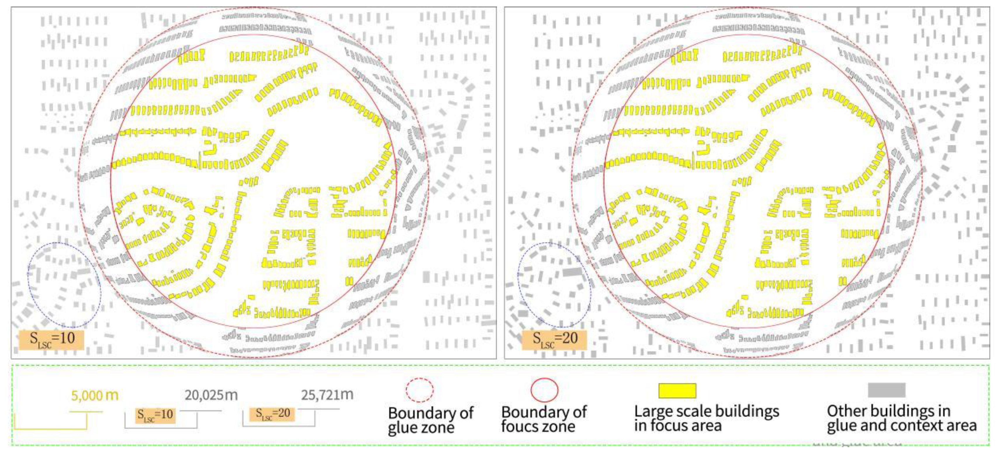
4.2.4. Parameter Selection and Evaluation

The superpixel aperture used in LSC superpixel segmentation clustering is 10, as shown in S_LSC in Table 1. Experiments have shown that the change in aperture size does not greatly affect the selection of typification but may change the establishment range of its typification area, which changes the subsequent relocation location of buildings. In Figure 17, the layout of the entire building is not very different. Additionally, the verification shows that, when using S_LSC = 20 for LSC superpixel segmentation clustering at the same level, the number of buildings after typification is 709, which is not far from the value of 799 of B_num in Table 1. Although there are some differences between the buildings in the blue rectangular box in the figure, the reason may be that the pore size used in clustering leads to the different division of typification areas, resulting in the difference between the buildings selected during relocation and the relocation location. However, its overall variable-scale visualization effect did not change much.

Then, for the design of the window neighborhood size of the median filter in the construction of typification regions (see S_m in Table 1), the size used this time is 29, which achieves good smoothing and simplification effects and can accurately maintain the relevant characteristics of the boundary. The manual selection of size in the operation process is very time-consuming. Further research may be needed to both intelligently select the sizes of the parameters and achieve better experimental results.

Then, for the LSC superpixel segmentation and placement of the typification area, the number of superpixel shapes designed is shown in T_num in Table 1. This paper is divided according to the proportion of superpixels, resulting in the proportion of the number of typified buildings relative to the number of original buildings. The hierarchical visualization is performed through a certain ratio relationship, which gives people a sense of progressive layers. Furthermore, we can select the typification proportion and draw the corresponding variable-scale map.

Additionally, for the establishment of the variable-scale model in this paper, the model size and radius are shown in R_G-C and R_F-G in Table 1. In the experiment, the size of the entire tile map and the designed radius are combined with the boundary treatment to plan a reasonable range of the focus area. Therefore, it is necessary to manually plan the corresponding position, and the focus area can be moved later. Combined with the corresponding visualization technology, the background loads the selected range for variable-scale visualization, which is not limited to a static map.

4.3. Comparison with Traditional Methods

Most electronic maps can be scrolled, magnified (zoomed in) and reduced (zoomed out). When browsing the map, users can scroll and magnify the view of interest [37]. As shown in Figure 18c, in the green circle in the middle, people can use the map roaming (scrolling mouse) operation to repeatedly check back and forth, which can easily distract the users. When magnifying and loading the map, users must retrieve data in the background, which requires a certain network speed and loading time. On this basis, the Baidu map, open layer, and other relevant network maps available on the current market have been designed using the eagle eye method to locally enlarge some areas. As shown in Figure 18b, users can move the map in the eagle eye frame to control the position display of the entire map and obtain the relative position of the large-scale thumbnail in the eagle eye on the overall map. However, for a large-scale map, the eagle eye thumbnail with a small border is a compromise. For a large-scale enlarged display, the display range of the eagle eye should change through the movement of the mouse to meet the needs of users. The variable-scale visual map display designed in this paper, as shown in Figure 18a, cannot meet the different needs of users for a single scale. However, it can enlarge the display elements to meet the needs of users without changing the overall layout of the original map elements, coordinate the local and overall relationship, and remedy the contradiction between users’ needs and complex map elements.

To better reflect the advantages of the proposed LSC superpixel-based typified buildings in this study over the traditional visualization, several typification parts are selected in Figure 18, i.e., the black and purple borders, which are partially integrated into Figure 19 for comparative analysis. First, for the parts surrounded by a black frame, Figure 19a is in the focus area, and with the surrounding transition area, the building layout shape is well preserved and has good continuity. In Figure 19b, region 1 is magnified at its eagle eye (blue border in Figure 18b), and only a small part of the content of the fixed size of the eagle eye can be displayed. In other words, in region 2, its periphery must be compared and identified in the original image and eagle eye image, which requires the user to scan and switch back and forth. In Figure 19c, the selection content is in the green magnification scale in Figure 18c, and only the buildings within the border are magnified, which makes the chain break at its boundary. Then, the purple border surrounds the part. In Figure 19a, it is in the transition area and background area. We can see the change in scale. The building layout is well connected and maintains the spatial distribution of the elements. In Figure 19b, for the purple part, because the eagle eye did not select this part of the building, there is no change effect. Lastly, in Figure 19c, due to the selection of the boundary of the scale change, some buildings are enlarged from the original region 1. Moving to region 2 causes disorder of the building layout and dislocation of the spatial position, which makes it difficult to identify the user information.

The F + G + C variable-scale models based on the superpixel and the two traditional methods evaluate the number, area, and building density of buildings in different display areas. As shown in

Table 2. Evaluation results of building quantity, area, and density by different methods.

Methods	Region	Number	Number (%)	Area	Area (%)	Density/A	Density/A (%)	Land Size
Orginal		1599		1,176,592		23.52%		8,699,840
F + G + C	Focus	398	−75.11%	283,163	−75.93%	21.62%	−8.10%	2,437,122
	Glue	567	−64.54%	169,269	−85.61%	17.47%	−25.74%	2,266,095
	Content	443	−72.30%	315,190	−73.21%	17.89%	−23.95%	3,994,619
Eagle eye	Inside eagle’s eye	61	−96.19%	119,048	−89.88%	33.50%	42.41%	506,553
	Eagle eye (outside)	1555	−2.75%	1,079,332	−8.27%	23.17%	−1.49%	8,193,613
View zoom in	Roaming area	279	−82.55%	393,176	−66.58%	21.08%	−10.38%	3,548,062
	Original base map	1062	−33.58%	660,728	−43.84%	22.83%	−2.95%	5,149,730

, the number of buildings is calculated through the connected domain, the unit of area is pixels, and the building density is the ratio of the total area of the building’s base to the occupied land area. Then, the reduction percentage of jumbled buildings in the original pictures compared using different methods is calculated. By analyzing Table 2, we obtain the following conclusions:

• With the subregional display, the buildings in the focal area, the buildings in the eagle eye, and the buildings in the enlarged view are enlarged, and their total number, area and density are less than the original, which can reduce the redundant data;
• The method of F + G + C based on superpixels uses partition display, and the percentage reduction in each parameter in each area is relatively balanced. Compared with the eagle eye area, which only has a small range to enlarge the building, the change is abrupt and sharp;
• Compared with the method of zooming in and displaying based on map roaming, the percentage reduction is relatively small, especially in the building density part, which does not play a role in removing the problem of complicated data volume;
• In other words, by using F + G + C based on superpixels for visualization, the number, area, and density of buildings are reduced by 70%, 78%, and 24% (the average of the three regions), which simplifies the massive building data. Taking all parameters into account, the data volume is reduced by 57%, and better visual effects are obtained.

4.4. Overlay with Original OSM Data

After using the method of variable-scale visualization, the results are restored to the map interface of OpenStreetMap, as shown in Figure 20 compared with the original building base map in Figure 13 in the experimental data; the number of gray buildings around the red dotted line, i.e., the context area, is reduced, and its shape is simplified. The glue scale transition area from the dotted line to the solid line can buffer the scale and overall interface changes, as well as absorb deformation. The yellow building in the red solid line is the original building, which is displayed by expanding and enlarging the scale to increase the focus of users. For a limited size screen, this method can improve the display requirements of users for different map elements, eliminate miscellaneous elements, and change the visual presentation.

5. Conclusions

In urbanization construction, to maximize the use benefit in limited land, roads tend to be narrow and dense, and the layout of buildings is denser and more concentrated. For the traditional single-scale map, it is difficult for users to accurately obtain the required data information. For this reason, the main implications of this paper are to use the F + G + C variable-scale visualization method based on superpixel typification to enrich the shortcoming that traditional methods are limited to vector map data sources and cannot process tile data structures, typify buildings through LSC superpixels, reduce the number of buildings based on maximum area reconstruction, and simplify the minimum bounding rectangle in the shape of buildings. Then, the F + G + C model is used to change the scale, maintain the layout of the overall building, take into account the readability of the reader and the recognition of data information, and comprehensively consider the number, area, and density of buildings. The reduction in redundant data is approximately 57% (average value of building quantity, area and density). The data obtained from OSM were used to evaluate this method, and the below conclusions were obtained from this study.

LSC superpixel segmentation and clustering are used when the traditional method cannot handle the grid data source. By maintaining the layout of buildings and considering map synthesis, the number of buildings is reduced, the shape of buildings is simplified, and the redundancy of data is reduced. Then, a variable-scale model is designed to improve the efficiency of user information acquisition and the visibility of maps.

1. The LSC superpixel processing method can maintain the distribution characteristics of the original buildings, reduce the number of buildings, and effectively finalize and simplify buildings in the grid tile data structure.

2. With the use of the F + G + C variable-scale method, the data redundancy in the case of a single scale is changed, but the original base map is retained to provide the user with reference to the corresponding geographical relationship, maintain the overall spatial position structure, facilitate the user’s identification, and improve the practicability. It is a simple and scientific map visualization method.

The proposed variable proportion method has some disadvantages, such as the manual selection of parameters, which may be random and time-consuming. The number of typified buildings is not limited to the three levels shown in this paper but can be changed according to the requirements of different users. Likewise, it is possible to change the range of the variable scale according to the different needs of users. In the process of visualization and boundary processing, it is important that we take into account the topological relationship between buildings to achieve a better display of the overall effect of the variable-scale method.

References

1. Robinson, A.C.; Demšar, U.; Moore, A.B.; Buckley, A.; Jiang, B.; Field, K.; Kraak, M.J.; Camboim, S.P.; Sluter, C.R. Geospatial big data and cartography: Research challenges and opportunities for making maps that matter. Int. J. Geogr. 2017, 3, 32–60. [Google Scholar] [CrossRef]
2. Bak, P.; Schaefer, M.; Stoffel, A.; Keim, D.A.; Omer, I. Density Equalizing Distortion of Large Geographic Point Sets. Cartogr. Geogr. Inf. Sci. 2009, 36, 237–250. [Google Scholar] [CrossRef]
3. Harrie, L.; Sarjakoski, L.T.; Lehto, L. A variable-scale map for small-display cartography. Int. Arch. Photogramm. Remote Sens. Spat. Inf. Sci. 2002, 34, 237–242. [Google Scholar]
4. Cheng, C.; Niu, F.; Cai, J.; Zhu, Y. Extensions of GAP-tree and its implementation based on a non-topological data model. Int. J. Geogr. Inf. Sci. 2008, 22, 657–673. [Google Scholar] [CrossRef]
5. Keil, J.; Edler, D.; Dickmann, F.; Kuchinke, L. Meaningfulness of landmark pictograms reduces visual salience and recognition performance. Appl. Ergon. 2019, 75, 214–220. [Google Scholar] [CrossRef]
6. Ai, T.; Ke, S.; Yang, M.; Li, J. Envelope generation and simplification of polylines using Delaunay triangulation. Int. J. Geogr. Inf. Sci. 2017, 31, 297–319. [Google Scholar] [CrossRef]
7. Huang, H.; Guo, Q.; Sun, Y.; Liu, Y. Reducing building conflicts in map generalization with an improved PSO algorithm. ISPRS Int. J. Geo-Inf. 2017, 6, 127. [Google Scholar] [CrossRef]
8. Haunert, J.H.; Sester, M. Area collapse and road centerlines based on straight skeletons. GeoInformatica 2008, 12, 169–191. [Google Scholar] [CrossRef]
9. Van Oosterom, P. Variable-scale topological data structures suitable for progressive data transfer: The GAP-face tree and GAP-edge forest. Cartogr. Geogr. Inf. Sci. 2005, 32, 331–346. [Google Scholar] [CrossRef]
10. Burghardt, D.; Cecconi, A. Mesh simplification for building typification. Int. J. Geogr. Inf. Sci. 2007, 21, 283–298. [Google Scholar] [CrossRef]
11. Gong, X.; Wu, F. A typification method for linear pattern in urban building generalization. Geocarto Int. 2018, 33, 189–207. [Google Scholar] [CrossRef]
12. Zhao, R.; Ai, T.; Wen, C. A Method for Generating Variable-Scale Maps for Small Displays. ISPRS Int. J. Geo-Inf. 2020, 9, 250. [Google Scholar] [CrossRef]
13. Anders, K.H. Level of detail generation of 3D building groups by aggregation and typification. In Proceedings of the 22nd International Cartographic Conference, Corûna, Spain, 9–16 July 2005. [Google Scholar]
14. Wang, L.; Guo, Q.; Liu, Y.; Sun, Y.; Wei, Z. Contextual building selection based on a genetic algorithm in map generalization. ISPRS Int. J. Geo-Inf. 2017, 6, 271. [Google Scholar] [CrossRef]
15. Sandro, S.; Massimo, R.; Matteo, Z. Pattern recognition and typification of ditches. In Advances in Cartography and GIScience; Springer: Berlin/Heidelberg, Germany, 2011; Volume 1, pp. 425–437. [Google Scholar]
16. Sester, M. Optimization approaches for generalization and data abstraction. Int. J. Geogr. Inf. Sci. 2005, 19, 871–897. [Google Scholar] [CrossRef]
17. Regnauld, N. Contextual building typification in automated map generalization. Algorithmica 2001, 30, 312–333. [Google Scholar] [CrossRef]
18. Dumont, M.; Touya, G.; Duchêne, C. Designing multiscale maps: Lessons learned from existing practices. Int. J. Cartogr. 2020, 6, 121–151. [Google Scholar] [CrossRef]
19. Yamamoto, D.; Ozeki, S.; Takahashi, N. Focus + Glue + Context: An improved fisheye approach for web map services. In Proceedings of the 17th ACM SIGSPATIAL International Conference on Advances in Geographic Information Systems, Seattle, WA, USA, 4–6 November 2009; ACM: New York, NY, USA, 2009. [Google Scholar]
20. Haunert, J.H.; Sering, L. Drawing road networks with focus regions. Vis. Comput. Graph. IEEE Trans. 2011, 17, 2555–2562. [Google Scholar] [CrossRef]
21. Li, Z.; Chen, J. Superpixel segmentation using linear spectral clustering. In Proceedings of the IEEE Conference on Computer Vision and Pattern Recognition, Boston, MA, USA, 7–12 June 2015; pp. 1356–1363. [Google Scholar]
22. Becker, B.; Six, H.W.; Widmayer, P. Spatial Priority Search: An Access Technique for Scaleless Maps. ACM 1991, 20, 128–137. [Google Scholar]
23. Ai, T.; Liang, R. Variable scale visualization of navigation electronic map. J. Wuhan Univ. 2007, 32, 127–130. [Google Scholar]
24. Gao, P.; Feng, Y. Realization of multiscale visualization of navigation electronic map. Jiangxi Surv. Mapp. 2010, 4, 35–37. [Google Scholar]
25. Takahashi, N. An Elastic Map System with Cognitive Map-based Operations. In International Perspectives on Maps and the Internet; Springer: Berlin/Heidelberg, Germany, 2008; pp. 73–87. [Google Scholar]
26. Shen, Y.; Ai, T.; Li, W.; Yang, M.; Feng, Y. A polygon aggregation method with globalfeature preservation using superpixel segmentation. Comput. Environ. Urban Syst. 2019, 75, 117–131. [Google Scholar] [CrossRef]
27. Shen, Y.; Ai, T.; He, Y. A new approach to line simplification based on image processing: A case study of water area boundaries. ISPRS Int. J. Geo-Inf. 2018, 7, 41. [Google Scholar] [CrossRef]
28. Shen, Y.; Ai, T.; Wang, L.; Zhou, J. A new approach to simplifying polygonal and linear features using superpixel segmentation. Int. J. Geogr. Inf. Sci. 2018, 32, 2023–2054. [Google Scholar] [CrossRef]
29. Huang, T.; Yang, G.; Tang, G. A fast two-dimensional median filtering algorithm. IEEE Trans. Acoust. Speech Signal Process. 1979, 27, 13–18. [Google Scholar] [CrossRef] [Green Version]
30. Shen, Y.L.; Ai, T.; Li, J.; Wang, L.; Li, W. A tile-map-based method for the typification of artificial polygonal water areas considering the legibility. Comput. Geosci. 2020, 143, 104552. [Google Scholar] [CrossRef]
31. Wood, J. Minimum Bounding Rectangle. In Encyclopedia of GIS; Shekhar, S., Xiong, H., Eds.; Springer: Boston, MA, USA, 2008. [Google Scholar] [CrossRef]
32. Fairbairmn, D.; Yaylor, G. Developing a Variable-ScaleMap Projection for Urban Areas. Comput. Geosci. 1995, 21, 1053–1064. [Google Scholar] [CrossRef]
33. Reichenbacher, T. The World in Your Pocket-To-wards a Mobile Cartography. In Proceedings of the the 20th Interna-tional Cartography Conference, Beijing, China, 6–10 August 2001. [Google Scholar]
34. Töpfer, F.; Pillewizer, W. The principles of selection, a means of cartographic generalization. Cartogr. J. 1966, 3, 10–16. [Google Scholar] [CrossRef]
35. David, B.; Garth, S. Pliable Display Technology for the Common Operational Picture; RTO Information Systems Technology Panel: Toronto, ON, Canada, 2004. [Google Scholar]
36. Srnka, E. The analytical solution of regular generalization in cartography. Int. Yearb. Cartogr. 1970, 10, 48–62. [Google Scholar]
37. Hollands, J.G.; Carey, T.T.; Matthews, M.L.; McCann, C.A. Presenting a graphical network: A comparison of performance using fisheye and scrolling views. In Proceedings of the Third International Conference on Human-Computer Interaction on Designing and Using Human-Computer Interfaces and Knowledge Based Systems, 2nd ed.; Elsevier Science Inc.: Amsterdam, The Netherlands, 1989; pp. 313–320. Available online: https://dl.acm.org/doi/abs/10.5555/92449.92489 (accessed on 21 May 2022).
Figure 1. Variable-scale representation based on POIs and roads. (a) Original POI map. (b)Variable-scale visualized POI map.
Ijgi 11 00505 g001
Figure 2. Variable-scale visualization flow chart of the polygonal building area.
Ijgi 11 00505 g002
Figure 3. Second-order neighborhood clustering using superpixels for buildings. (a) Original buildings tile map. (b) Buildings connection boundary diagram. (c) Superpixel neighborhood graph. (d) Typicification area of buildings.
Ijgi 11 00505 g003
Figure 4. Median filtering in typification regions of buildings. (a) original shape. (b) Median filter size 9 results. (c) Median filter size 19 results. (d) Median filter size 29 results.
Ijgi 11 00505 g004
Figure 5. Construction of typification areas of buildings with the median filter.
Ijgi 11 00505 g005
Figure 6. LSC superpixel segmentation is used to segment the typification areas of the building. (a) Small Aperture superpixel Blocking Results. (b) Big Aperture superpixel Blocking Results.
Ijgi 11 00505 g006
Figure 7. Division of typification areas of buildings.
Ijgi 11 00505 g007
Figure 8. Relocation of buildings based on the maximum area. (a) Typified buildings of small aperture superpixel. (b) Typified buildings of big aperture superpixel.
Ijgi 11 00505 g008
Figure 9. Binary image boundary search.
Ijgi 11 00505 g009
Figure 10. Simplification of the building shapes.
Ijgi 11 00505 g010
Figure 11. Variable-scale models. (a) Original base drawing. (b) F + G + C variable-scale model. (c) Adaptive variable-scale model. (d) Scale change curve of F + G + C model.
Ijgi 11 00505 g011
Figure 12. Removing the boundary conflicts.
Ijgi 11 00505 g012
Figure 13. Experimental data.
Ijgi 11 00505 g013
Figure 14. Multilevel variable-scale visualization results of buildings. (a) Variable-scale results for building typified level 1; (b) Variable-scale results for building typified level 2; (c) Variable-scale results for building typified level 3.
Ijgi 11 00505 g014
Figure 15. Multicore adaptive variable-scale visualization of buildings.
Ijgi 11 00505 g015
Figure 16. Consider topology and legibility. (a) Original topology error map. (b) Topology correction results.
Ijgi 11 00505 g016
Figure 17. Typification comparison of different aperture superpixel LSC sizes.
Ijgi 11 00505 g017
Figure 18. Comparison with traditional methods. (a) The result of variable-scale map. (b) The result of eagle eye map. (c) The result of roaming Map.
Ijgi 11 00505 g018
Figure 19. Comparison of details of different variable-scale methods in different regions. (a) Comparison area in the variable-scale map. (b) Comparison area in the eagle eye map. (c) Compare area in the roaming map.
Ijgi 11 00505 g019
Figure 20. Overlay with original OSM data.
Ijgi 11 00505 g020