Application of Social Network Analysis in the Economic Connection of Urban Agglomerations Based on Nighttime Lights Remote Sensing: A Case Study in the New Western Land-Sea Corridor, China

Abstract

Nighttime lights remote sensing has a significant advantage in exploring the economic development of cities. Based on nighttime lighting data, this study employed spatial direction analysis, exploratory spatial data analysis, and social network analysis to explore the spatial characteristics of economic development and analyzed the economic connection network structures within urban agglomerations in the New Western Land-sea Corridor (NWLSC) in western China. The results show that the spatial pattern of the Tianshan North slope urban agglomeration, Guanzhong Plain urban agglomeration, and Lanzhou–Xining urban agglomeration shrank, while other urban agglomerations expanded. The city economy of the Chengdu–Chongqing urban agglomeration (CCUA) and the Beibu Gulf urban agglomeration varied dramatically according to a LISA space-time transition analysis, which indicates a strong spatial dependence between cities in the local space. Within urban agglomerations, the economic connection between cities increased significantly, and central cities were at the core of the network and significantly influenced other cities. Among the urban agglomerations, economic connections among neighboring urban agglomerations in geographic space increased during the study period. The CCUA gradually developed into the center of the economic network in the NWLSC. Network density positively influenced economic connections. The degree centrality, closeness centrality, and betweenness centrality significantly enhanced the economic connections between city agglomerations. The study’s conclusions and methods can serve as the policy support for the cooperative development of urban agglomerations in NWLSC serve as a guideline for the development of other economically underdeveloped regions in the world.

1. Introduction

With constant progress made in transportation technologies and systems, the economic ties between Chinese cities are becoming increasingly close. A city, as the economic and cultural center of a region, while fueling its development with products and services absorbed through economically connected networks, is also giving impetus to the development of its surrounding areas [1]. Urban development has advanced quickly in China’s western area. However, due to limitations in natural resources and transportation, there are still problems such as low and unbalanced urbanization development. Strengthening the economic connection between cities is an urgent issue at present. The Chinese government launched a strategy for the New Western Land-Sea Corridor (NWLSC) in 2019, aiming to promote openness to the outside world and implement various measures to promote inter-city economic connection [2,3]. Therefore, a thorough analysis of economic development trends and inter-city economic connections in the western area of China is extremely important for research.

As an important part of geographical research, regional economic connections not only facilitate the exchange of resources between different geographical locations but also promote communication and sharing of information and technologies [4]. In 1946, Zipf was the first to introduce the gravity model into research on regional interactions, providing the theoretical basis for studying the economic interaction between cities [5]. Many scholars have researched economic connections between cities examining areas such as theoretical innovation, model optimization, and empirical analysis, and have achieved fruitful results [6,7,8,9,10]. Ye et al. [11] analyzed the economic network structure and strength of urban agglomerations based on methods of the modified gravity model and social networks analysis (SNA). Jin et al. [12] selected Guangdong Province as their study area and used SNA and a spatial econometric model to examine the structure and influencing factors of the economic network. Based on the data of China’s top 500 enterprises, Zhao et al. [13] analyzed China’s urban economic connection network and found that the urban network and agglomeration economy has a positive impact on urban economic growth. At present, research on the economic connections between cities mainly focuses on the measurement of economic connections [14], improvements to the gravity model [15], and exploration of the driving mechanisms [16]. With the development of big data technology, big data from multiple sources including images of nighttime light (NTL) remote sensing, information flow [17,18], traffic flow [19,20], human mobility [21], etc. have opened new directions for research on the economic connections between cities, which can be used to more accurately reveal the inherent mechanisms. In addition, with growing differences between inter-city economic activities and increasing complexity of the economic connections between urban subjects, research on the spatial structure of economic connection [22] has become an important means to explore the status quo of economic development. Research methods such as gravity models [23,24], potential models [25], spatial structure indexes [26], SNA [27,28], etc. are being increasingly adopted.

However, there are inadequacies in the selection of study areas and data applications in the study of economic connections. First, current research on regional economic connection mainly focuses on cities [12,16], along an economic belt [29], and developed areas [30], while scarce research is dedicated to discussions on urban agglomerations and economically underdeveloped areas. In the advanced stages of city development, urban agglomerations represent the highest form of spatial organization and have a clear radiation-driven effect on the neighboring cities [31]. Additionally, the emergence and growth of urban agglomerations are facilitated by inter-city communication, cooperation, and labor division [32]. It is consequently of considerable significance to analyze economic development patterns and economic spatial connections from the perspective of urban agglomerations. Second, existing studies of economic connection have mainly adopted single indicator data such as population or GDP, which cannot objectively reflect the real situation. The economic connections between regions are complex and consist of goods, labor, capital, technology, and information. In addition, there are problems such as difficulties in obtaining socioeconomic data from lower-level administrative regions and underdeveloped cities, which limits the scope for detailed analysis.

Since changes in NTL images can reflect movements in human activity, this provides a fresh perspective for studying social activities. Croft first developed research using NTL images in 1978 [33], and many scholars have applied NTL data to studies in different fields. The objectivity and stability of this method have solved the problem of inconsistent statistical caliber existing in traditional statistical data. NTL data have been widely used in spatial structure analysis [34,35], economic development assessment [36,37], environmental monitoring [38], and population estimation of a city [39,40]. Numerous studies in the area of economic assessment have shown a significant relationship between the NTL and economic indicators such as GDP [41]. In statistically deficient areas, estimation based on NTL can enhance the quality of socioeconomic data. Currently, NTL images are frequently used as a measure of regional poverty [42], imbalance of city economic development [43], etc. Chen et al. [44] investigated the potential of the digital economy using NTL remote sensing data. Based on NTL data, Cui et al. [45] analyzed the nighttime economy’s development characteristics in China. Additionally, NTL images are gradually becoming more varied and significantly improved in terms of radiation resolution as technology advances, which can reveal economic activity more accurately. However, few studies use NTL data to analyze urban economic connections, according to the literature review above. Based on the benefits of NTL data for spatial analysis, the issue of missing data may be resolved to some extent when examining the economic trends and connections among urban agglomerations, and the reliability of research findings can be increased.

Addressing the limitations of previous research on economic connections, this study focused on the urban agglomerations in the NWLSC, where the economy and urbanization of most cities need to be improved and the strengthening of economic connections is an urgent issue. We analyzed the evolutionary trends in the economic development of urban agglomerations and the spatial structural characteristics of the economic connection network, taking advantage of the availability and objectivity of NTL data. The main purpose of this study is to explore the economic development trends in economically underdeveloped regions of China, and then analyze the economic connection network and its spatial structure within and between urban agglomerations. This study’s potential value is to offer empirical support for relevant policy-making and to promote urban and economic growth in the NWLSC and other areas of the world, particularly those that are economically undeveloped.

2. Materials and Methods

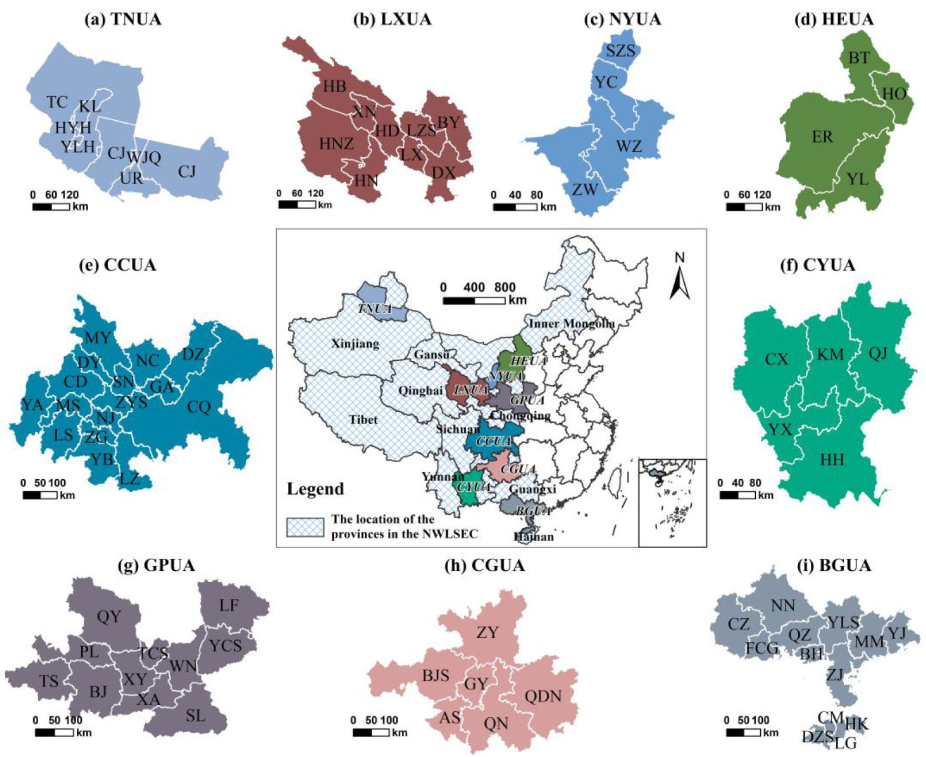
2.1. Study Area

The NWLSC strategy covers a total of 13 provinces (autonomous regions and municipalities) including Inner Mongolia, Xinjiang, Tibet, Qinghai, Shaanxi, Ningxia, Yunnan, Sichuan, Gansu, Guangxi, Hainan, and Chongqing, as well as Zhanjiang City, Guangdong Province. These places differ greatly from each other in terms of economic development and resource endowment. By the end of 2020, this region achieved a GDP of 21.33 trillion Yuan and had a total resident population of about 382 million. The NWLSC organically connects the “21st Century Maritime Silk Road Economic Belt” and the “Silk Road Economic Belt”, which are of great significance in promoting the high-quality development of China’s economy. According to the strategic planning for the development of urban agglomerations in China, there are nine urban agglomerations in the NWLSC. The establishment of urban agglomerations promotes the flow of capital, logistics, and other production factors, and radiates the growth of adjacent cities.

Table 1. The information on urban agglomerations in the NWLSC.

Urban Agglomeration	City	Symbol	Urban Agglomeration	City	Symbol
Ningxia urban agglomeration along the Yellow River	Yinchuan	YC	Hohhot–Baotou–Ordos–Yulin urban agglomeration	Erdos	ER
	Wuzhong	WZ		Baotou	BT
	Shizuishan	SZS		Hohhot	HO
	Zhongwei	ZW		Yulin	YL
Guanzhong Plain urban agglomeration	Xi’an	XA	Beibu Gulf urban agglomeration	Nanning	NN
	Xianyang	XY		Zhanjiang	ZJ
	Weinan	WN		Maoming	MM
	Qingyang	QY		Qinzhou	QZ
	Baoji	BJ		Yulin	YLS
	Tongchuan	TCS		Yangjiang	YJ
	Tianshui	TS		Beihai	BH
	Pingliang	PL		Haikou	HK
	Shangluo	SL		Fangchenggang	FCG
	Yuncheng	YCS		Danzhou	DZS
	Linfen	LF		Chongzuo	CZ
Chengdu–Chongqing urban agglomeration	Chengdu	CD	Lanzhou–Xining urban agglomeration LXUA	Lanzhou	LZS
	Dazhou	DZ		Xining	XN
	Deyang	DY		Dingxi	DX
	Guangan	GA		Haidong	HD
	Leshan	LS		Baiyin	BY
	Luzhou	LZ		Haibei	HB
	Meishan	MS		Hainan	HNZ
	Mianyang	MY		Huangnan	HN
	Nanchong	NC		Linxia	LX
	Neijiang	NJ	central Guizhou urban agglomeration	Guiyang	GY
	Suining	SN		Zunyi	ZY
	Yaan	YA		Qiannan	QN
	Yibin	YB		Qiandongnan	QDN
	Chongqing	CQ		Anshun	AS
	Ziyang	ZYS		Bijie	BJS
	Zigong	ZG	Tianshan North slope urban agglomeration	Urumqi	UR
central Yunnan urban agglomeration	Kunming	KM		Changji	CJ
	Qujing	QJ		Karamay	KL
	Yuxi	YX		Tacheng	TC
	Chuxiong	CX		Huyanghe	HYH
	Honghe	HH		Yili	YLH
				Wujiaqu	WJQ

and Figure 1 show the information on urban agglomerations and the location of the NWLSC, respectively.

2.2. Data Sources and Preprocessing

The research data of this study include economic statistics, NTL data, and administrative boundaries data. The economic statistics were obtained from the China City Statistical Yearbook. The administrative boundaries data are from the Data Center for Resources and Environmental Sciences, Chinese Academy of Sciences. This study used the annual NTL data produced by Chen et al. [46]. This dataset was produced based on the DMSP/OLS and NPP/VIIRS remote sensing images, which show good accuracy and temporal consistency. First, the remote sensing image data were processed using the auto encoder model and a cross-sensory calibration model. Then, an extended time series of nighttime light data was obtained by training the model. The dataset of nighttime light data uses the WGS84 coordinate system with a spatial resolution of 500 m. Based on this dataset, Li et al. [47] analyzed the characteristics of urbanization evolution in three major urban agglomerations in China.

Referring to previous studies [48,49], the NTL index, defined as the sum of all pixel values in a region of an image [50], is taken to characterize economic development. First, we cropped the NTL images based on the administrative boundary vector data of the urban agglomerations. On this basis, the NTL image was reprojected and resampled. Second, we extracted the total value of NTL based on the administrative division boundaries, and we used the sum of the DN values within a city-level unit.

2.3. Methodology

Combining nighttime light data and statistics data, this study analyzes the evolutionary characteristics of economic development and economic coordination trends of urban agglomerations from global and micro perspectives. The framework of our study is shown in Figure 2. First, we use directional analysis, global Moran’s I, and LISA space-time transition to analyze the economic development characteristics of urban agglomerations in the NWLSC. The directional analysis can reveal the direction and center of economic development from an overall perspective. The global Moran’s I shows the spatial aggregation characteristics of economic development. The LISA space-time transition reveals the dynamic characteristics of economic development from a local perspective. Second, we develop a modified gravity model using statistics and NTL data to assess the economic connections within and between urban agglomerations. The modified gravity model can show detailed characteristics of the economic connection intensity and coordinated development between urban agglomerations. Third, based on the constructed economic connection network, we use social network analysis to explore the structural characteristics of the network and to analyze the spatial radiation effects of core cities. Fourth, using both individual network and overall network perspectives, we apply regression analysis to explore how network structure affects economic connection strength. This analysis contributes to the formulation of a more precise policy for coordinated, high-quality development.

2.3.1. Directional Analysis

The directional analysis can explain the spatial distribution and changing trends in the production factors. Combining the advantages of NTL images for reflecting economic development, we use directional analysis to explore economic trends in spatial extent and spatial direction [51,52] and the spatial dynamics mechanism. The calculation is shown in Equation (1):

$$X_t=\frac{{\displaystyle \sum _{i=1}^{n}NT{L}_i{x}_i}}{{\displaystyle \sum _{i=1}^{n}NT{L}_i}}; Y_t=\frac{{\displaystyle \sum _{i=1}^{n}NT{L}_i{y}_i}}{{\displaystyle \sum _{i=1}^{n}NT{L}_i}}$$

(1)

where (X_t, Y_t) denotes the coordinates of the economic gravity in year t; (x_i, y_i) denotes the spatial location of the city i; NTL_i represents the NTL index of the city i; and n is the number of cities in the urban agglomeration.

2.3.2. Heterogeneity Analysis of Economic Trends

The global Moran’s I reveal the dependence and heterogeneity in the economic development of urban agglomerations from an overall perspective [42,53]. Based on the NTL index, we explore the heterogeneity of economic development. The calculation is shown in Equation (2):

$$Mora{n}^{\prime }sI=\frac{n{\displaystyle \sum _{i=1}^n{\displaystyle \sum _{j=1}^n{w}_{ij}\left(NT{L}_i-\overline{NTL}\right)\left(NT{L}_j-\overline{NTL}\right)}}}{{\displaystyle \sum _{i=1}^n{\left(NT{L}_i-\overline{NTL}\right)}^2\left({\displaystyle \sum _{i=1}^n{\displaystyle \sum _{j=1}^n{w}_{ij}}}\right)}}$$

(2)

where W_ij is the spatial weight matrix; NTL_i and NTL_j are the NTL index of the city i and j, respectively; $\overline{NTL}$ is the mean value of the NTL index, and n is the number of cities in the urban agglomeration.

2.3.3. LISA Space-Time Transition Analysis

Local Indicators of Spatial Association (LISA) is employed to investigate the spatiotemporal dynamics of economic development [54,55]. The spatiotemporal tendencies of economic development of urban agglomerations evolving on a local scale can be reflected by the LISA space-time transition [56,57,58]. Therefore, we study the economic development characteristics of urban agglomerations from the perspective of local dynamic changes based on the NTL index. Equations (3) and (4) express the calculation of path length and curvature, respectively:

$$d=\frac{n{\displaystyle \sum _{t=1}^{T-1}d\left(L_{i,t},L_{i,t+1}\right)}}{{\displaystyle \sum _{i=1}^n{\displaystyle \sum _{t=1}^{T-1}d\left(L_{i,t},L_{i,t+1}\right)}}}$$

(3)

$$f=\frac{{\displaystyle \sum _{t=1}^{T-1}d\left(L_{i,t},L_{i,t+1}\right)}}{d\left(L_{i,1},L_{i,T}\right)}$$

(4)

where d denotes the value of path length; f denotes the value of path curvature; n is the number of prefecture-level units; T represents the study duration; d (L_i,t, L_i,t+1) is the distance that the NTL index of the city i moves from time t to t + 1 in the Moran scatter plot; and d (L_i,t, L_i,T) is the distance that the NTL index of the city i moves from time t to T in the Moran scatter plot. In addition, the greater the d, the more significant the dynamic evolution of the economy. The greater the f, the stronger the economic dependence of the urban agglomeration.

2.3.4. Economic Connections Analysis

Due to the differences in resource endowments, the economic connections between cities are imbalanced. We construct a modified gravitational model to calculate the economic connection between cities based on NTL data and statistical economic data [16,59], as shown in Equations (5) and (6). The modified gravity model reveals the directionality of economic factor flows between cities:

$$C_{ij}=K_{ij}\frac{E_i\times E_j}{D_{ij}^2}$$

(5)

$$k_{ij}=\frac{NT{L}_i}{NT{L}_i+NT{L}_j}$$

(6)

where C_ij is the economic connection between city i and j; and E_i and E_j are the economic development quality of city i and j, respectively. NTL_i and NTL_j are the NTL index of the city i and j; k_ij is the modified gravitational coefficient; D_ij represents the spatial distance between city i and j; and C_i is the total economic connection of city i.

The economic development quality is a comprehensive system with diverse, diversified, and multidimensional components [60]. Economic growth is no longer simply pursuing the growth of GDP and other macroeconomic indicators but requires efficient, stable, and sustainable development [61]. There is variability in the economic development and economic scale of cities in the NWLSC. Referring to the studies of Kong et al. [62] and Gan et al. [24], we constructed a dimensions of economic development quality indicator system based on the principles of scientificity and systematicity. The indicator system includes economic scale, economic vitality, residents’ income level, and public finance income and expenditure (

Table 2. The economic development quality indicator system.

Primary Indicators	Secondary Indicators	Units
Economic scale	Gross regional product	10,000 Yuan
Economic vitality	Persons employed in various units at year-end	10,000 persons
	Total retail sales of consumer goods	10,000 Yuan
	Amount of foreign capital actually utilized	USD 10,000
Residents’ income level	Average wage of employed staff and workers	Yuan
	household saving deposits	10,000 Yuan
Public finance income and expenditure	General public budget revenue	10,000 Yuan
	General public budget expenditure	10,000 Yuan

). Further, we use the entropy method to calculate the economic development quality.

The entropy method is used to determine the index weights by analyzing the correlation degree among the indexes and then calculating the comprehensive economic system [63]:

Positive indicator:

$$X_{ij}^{\prime }=\frac{x_{ij}-\min \left(x_{ij}\right)}{\max \left(x_{ij}\right)-\min \left(x_{ij}\right)}$$

(7)

Negative indicator:

$$X_{ij}^{\prime }=\frac{\max \left(x_{ij}\right)-x_{ij}}{\max \left(x_{ij}\right)-\min \left(x_{ij}\right)}$$

(8)

where X_ij denotes the value of indicator j in the year i; max(x_ij) denotes the maximum value of indicator X_ij; min(x_ij) represents the minimum value of X_ij; and $X_{ij}^{\prime }$ is the standardized value of X_ij. Then:

$$p_{ij}^{\prime }=\raisebox{1ex}{$\left(1+x_{ij}\right)$}\!\left/ \!\raisebox{-1ex}{${\displaystyle \sum _{i=1}^n\left(1+x_{ij}\right)}$}\right.$$

(9)

$$e_{ij}=-\frac{1}{\ln m}{\displaystyle \sum _{i=1}^n{p}_{ij}\times \ln \left(p_{ij}\right)}$$

(10)

where p_ij is the weight of indicator value of indicator j in the year i, and e_ij represents the entropy value of indicator j in the year i. Then:

$$w_{ij}=\frac{1-e_{ij}}{{\displaystyle \sum _{j=1}^m\left(1-e_{ij}\right)}}$$

(11)

$$U_{ij}={\displaystyle \sum _{i=1,j=1}^{n,m}{x}_{ij}^{\prime }}\times w_{ij}$$

(12)

where w_ij is the weight of the index j of city i, and U_ij is the comprehensive score of the system.

2.3.5. Structure Analysis of Economic Network

The SNA method can reveal the spatial structure of a network from an overall and individual perspective [64]. The formulae and explanation of relevant indicators for SNA are shown in

Table 3. Formulae and explanation of indicators for SNA.

Index	Meaning	Formula	Explanation of Formula
Network density	Network density reflects the degree of connection between the nodes. The greater the degree of closeness, the closer the economic connection between the network nodes [65].	$D=\frac{L}{N\times \left(N-1\right)}$	D is the network density; L denotes the number of relationships owned; N × (N − 1) denotes the maximum number of possible relationships.
Degree centrality	Degree centrality measures the weight of a node’s position in the overall network. If a node is related to many other nodes, it indicates that the node is in a more central position. The higher the degree centrality, the more critical position the node is in [66].	$D_e=\frac{N}{N-1}$	De is the degree centrality of node i; N denotes the number of network nodes.
Closeness centrality	Closeness centrality indicates the degree to which a node in the network is not controlled by other nodes. The higher the closeness centrality value, the more likely the node is at the center [67].	$C_{A{P}_i}^{-1}={\displaystyle \sum _{i=1}^n{d}_{ij}}$	$C_{A{P}_i}^{-1}$ denotes the closeness centrality and dij represent the distance between two nodes.
Betweenness centrality	Median centrality means the ability of a node to control other nodes. If a node is in the path of other nodes in the network, then the node has high mesoscopic centrality [68].	$BC\left(n_i\right)={\displaystyle \sum _{s\ne i\ne t}\frac{n_{st}^i}{g_{st}^i}}$	BC(ni) is the betweenness centrality; gst is the number of shortest paths from node s to node t; $n_{st}^i$ is the number of shortest paths through node i among the gst shortest paths from node s to node t.
Structural hole	The structural hole is formed when there is no direct connection between two additional actors connected by one actor in the network [69]. Four indicators make up the structural hole index: effective size, efficiency, constraint, and hierarchy. This study examines the structural change feature of economic connection networks in each urban agglomeration by focusing on effective size and efficiency.	$ES={\displaystyle \sum _j\left(1-{\displaystyle \sum _q{p}_{iq}{m}_{jq}}\right)},q\ne i,j$	ES represents the effective size of node i; j is all points connected to node i; q is the third party except i or j; pin and mjq represent the redundancy between node i and point j; p and n are the proportion of the relationship that actor i puts into q; mjq is the marginal strength of the relationship from j to q, which is equal to the value of the relationship taken from j to q divided by the maximum value in the relationship from j to other points.

. Taking the cities of urban agglomerations as network nodes, this study regards the economic connection between cities as network edges and considers the direction of economic connection to build an urban economic connection network. The SNA method is adopted to explore the spatial structure characteristics and evolutionary laws of economic networks.

The cohesion subgroups approach is used in this study to achieve group identification of economic networks. The actual or possible relationships of each node in the network are revealed by the cohesion subgroups. The term “cohesive subgroup” refers to a group in which the economic relationships between nodes in the network are particularly intimately correlated [70].

The core–edge structure is employed in this study to split the nodes of the economic connection network. Space network nodes are divided into core actors and edge actors by the core–edge structure. Core players who are closely linked form cohesive groupings, whereas marginal actors are less related [71].

2.3.6. Structural Effect Analysis

Numerous elements influence the growth of the economic connectivity network. We discuss the impact of network structure on the economic connection, focusing on both the overall and individual network structure. In the examination of the total network structure effect, the dependent variable is the mean value of the economic connection, and the independent variables are network density, network hierarchy, and network efficiency to carry out regression analysis. For the effect analysis of individual network structures, the economic connection is the dependent variable and the network centrality index is the independent variable.

3. Results

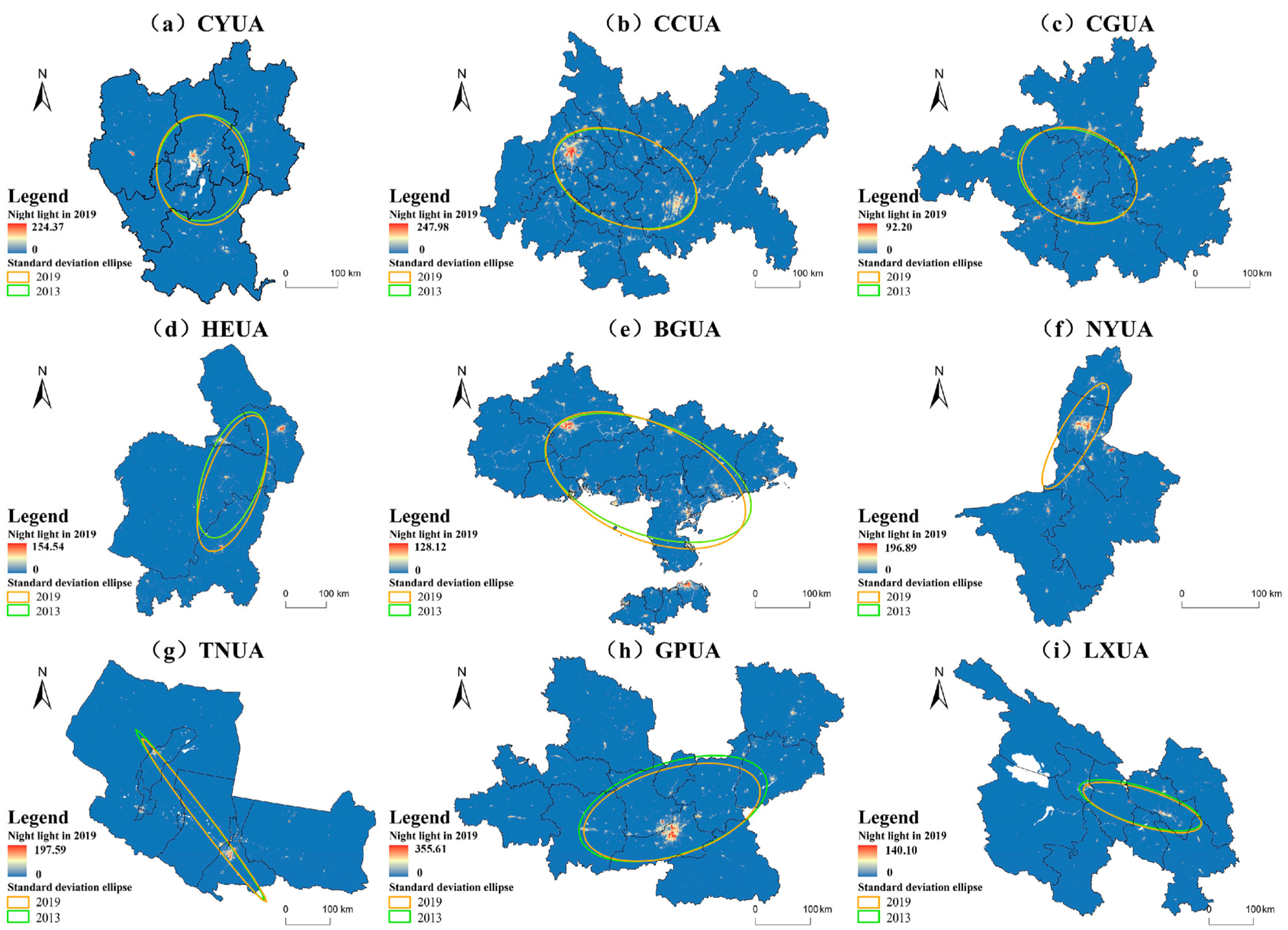
3.1. Economic Distribution of Urban Agglomeration

Figure 3 depicts the economic spatial pattern evolution of urban agglomerations in the NWLSC between 2013 and 2019. Each urban agglomeration’s core cities have a sizable NTL index. While the other urban agglomerations have a spatial pattern structure with the province’s capital city at the center, the CCUA and BGUA have a “double-core agglomeration” economic structure. The area of the standard deviation ellipse was higher in the CYUA, CCUA, CGUA, HEUA, BGUA, and NYUA, indicating that the economic development shows a radiation effect and that economic scale achieves growth. The area of standard deviation ellipse was lower for the GPUA, TNUA, and LXUA, which means that the agglomeration of urban economies increased. Considering shape of the standard deviation ellipse, HEUA, NYUA, TNUA, and LXUA showed a flattened shape, indicating economic development occurring in a belt shape. In terms of economic spatial distribution, the CCUA, CGUA, BGUA, LXUA, and TNUA had a “northwest–southeast” distribution, whilst HEUA, NYUA, GPUA, and CYUA had a “northeast–southwest” distribution.

According to

Table 4. Standard deviation ellipse changes in 2013 and 2019.

Urban Agglomeration	Year	Barycentric Coordinates	Spatial Variation	Azimuth	Moving Direction of Barycentric	Spatial Growth Rate
NYUA	2013	(106°11′ E, 38°39′ N)	Expansion	38.15	Southwest	1.48%
	2019	(106°10′ E, 38°35′ N)		39.14
GPUA	2013	(108°98′ E, 34°65′ N)	Shrinkage	78.69	Southwest	−12.29%
	2019	(108°96′ E, 34°59′ N)		79.71
TNUA	2013	(86°49′ E, 44°53′ N)	Shrinkage	122.25	Southeast	−0.89%
	2019	(86°64′ E, 44°44′ N)		122.13
HEUA	2013	(110°18′ E, 39°86′ N)	Expansion	33.90	Southwest	3.66%
	2019	(110°17′ E, 39°67′ N)		32.10
CCUA	2013	(105°31′ E, 30°09′ N)	Expansion	105.95	Northeast	0.91%
	2019	(105°32′ E, 30°10′ N)		107.42
LXUA	2013	(103°11′ E, 36°25′ N)	Shrinkage	101.91	Northeast	−5.84%
	2019	(103°16′ E, 36°21′ N)		102.40
CYUA	2013	(102°90′ E, 24°82′ N)	Expansion	166.55	Southwest	2.48%
	2019	(102°89′ E, 24°78′ N)		167.21
CGUA	2013	(106°67′ E, 26°93′ N)	Expansion	107.88	Northeast	0.55%
	2019	(106°71′ E, 26°94′ N)		109.06
BGUA	2013	(109°72′ E, 21°86′ N)	Expansion	112.25	Southwest	2.11%
	2019	(109°67′ E, 21°82′ N)		115.76

, the BGUA had the maximum deflection angle, rotating from 112.25 to 115.76 in the direction of rotation. The TNUA had the smallest deflection angle, with a rotation from 122.25 to 122.13 radially. The economic gravity of each urban agglomeration shifted in different directions from 2013 to 2019. In the CYUA, HEUA, BGUA, NYUA, and GPUA, the economic center of gravity shifted to the southwest. The economic gravity of the CCUA, CGUA, and LXUA migrated to the northeast, but the economic gravity of the TNUA changed to the southeast. This shows that the economic scale and economic structure of urban agglomerations have changed with economic development.

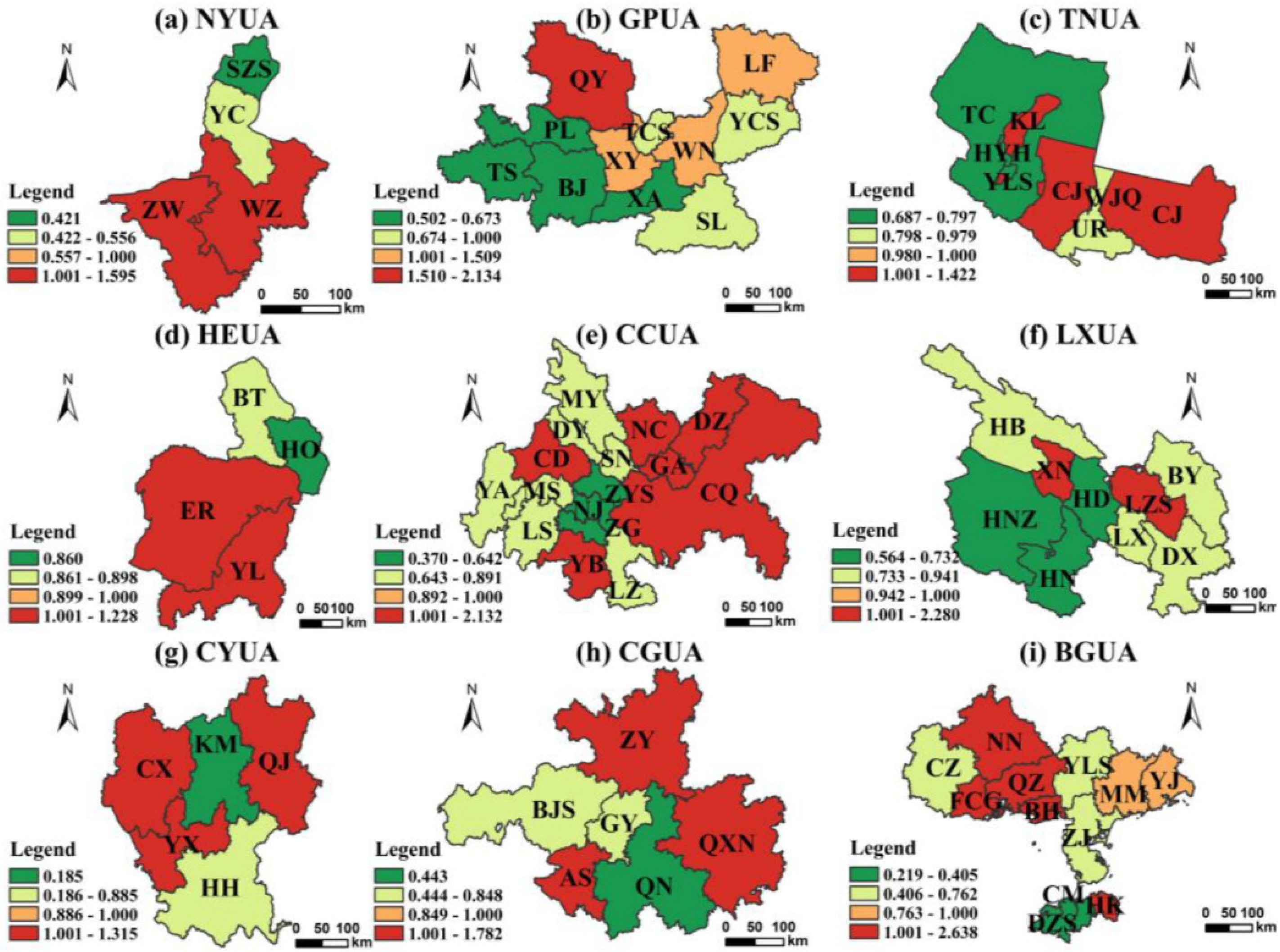
3.2. Economic Heterogeneity of Urban Agglomerations

The Moran’s I values of economics in the urban agglomerations are shown in

Table 5. Moran’s I of economics in urban agglomerations in 2013, 2016, and 2019.

Urban Agglomeration	Year	Global Moran’s I	Z-Score	p-Value
NYUA	2013	−0.5278	−0.6869	0.4922
	2016	−0.6067	−1.1030	0.2700
	2019	−0.6132	−1.1113	0.2665
GPUA	2013	−0.1034	−0.0206	0.9836
	2016	−0.1195	−0.1151	0.9084
	2019	−0.0899	0.0564	0.9550
TNUA	2013	−0.1659	−0.0626	0.9501
	2016	−0.1314	0.0302	0.9759
	2019	−0.0915	0.1301	0.8965
HEUA	2013	0.4582	1.3002	0.1935
	2016	−0.3983	−0.1354	0.8923
	2019	−0.3633	−0.0535	0.9574
CCUA	2013	0.0091	0.4406	0.6595
	2016	0.0123	0.4541	0.6497
	2019	0.0161	0.4761	0.6340
LXUA	2013	−0.5051	−1.6594	0.0970
	2016	−0.5139	−1.6186	0.1055
	2019	−0.5126	−1.6674	0.0954
CYUA	2013	−0.5077	−1.1992	0.2305
	2016	−0.5148	−1.2755	0.2021
	2019	−0.4137	−0.7569	0.4491
CGUA	2013	−0.4725	−1.2037	0.2287
	2016	−0.2971	−0.4286	0.6682
	2019	−0.5899	−0.3967	0.6916
BGUA	2013	0.2975	1.2925	0.1962
	2016	0.2610	1.1914	0.2335
	2019	0.3917	1.6024	0.1091

. The Moran’s I values generally change each year. The Z-score and p-value results failed to pass the significance test, suggesting that urban agglomerations’ economic growth occurs at random. The Moran’s I values for the CCUA and BGUA are consistently positive. HEUA’s Moran’s I value was positive in 2013 but negative in 2016 and 2019. The Moran’s I values for the CYUA, CGUA, CPUA, LXUA, NYUA, and TNUA are all negative. A thorough analysis of the above shows that each urban agglomeration’s economic growth is spatially independent and has spillover consequences.

3.3. Economic Space-Time Transition of Urban Agglomerations

Figure 4 shows the LISA time path length of economic development in each city. The values for Kunming, Lingao, and Chengmai are comparatively low, indicating that the spatial structure of economic development is more stable. Qinzhou, Xining, Nanning, Qingyang, and Chongqing have lengthy values, indicating that the spatial structures of economy development has changed dramatically. A higher proportion of cities with LISA time path lengths greater than 1 in the CCUA and BGUA, indicates that the economic development pattern shows a significant pattern of change over time. The CCUA and BGUA had a larger number of cities and a larger economic scale, and the movement of the production factors between cities increased. The GPUA and HEUA had the lowest percentage of cities with a LISA time path length greater than 1, which indicates that economic development has a rather constant regional structure.

Figure 5 shows the LISA time path curvature of economic development in each city. Each city had a LISA time path curvature value greater than 1, indicating a significant geographical dependence on economic development. In Kunming, Baiyin, Anshun, and Xining, higher values are seen, indicating a significant dynamic change and connectivity between these cities and others nearby. Nanning, Qinzhou, and Changji all had lower scores, indicating that the spatial reliance on cities’ economic development is generally stable. Additionally, the mean values of curvature of CYUA and LXUA were the highest, and the interconnections among their cities’ economic development were the strongest.

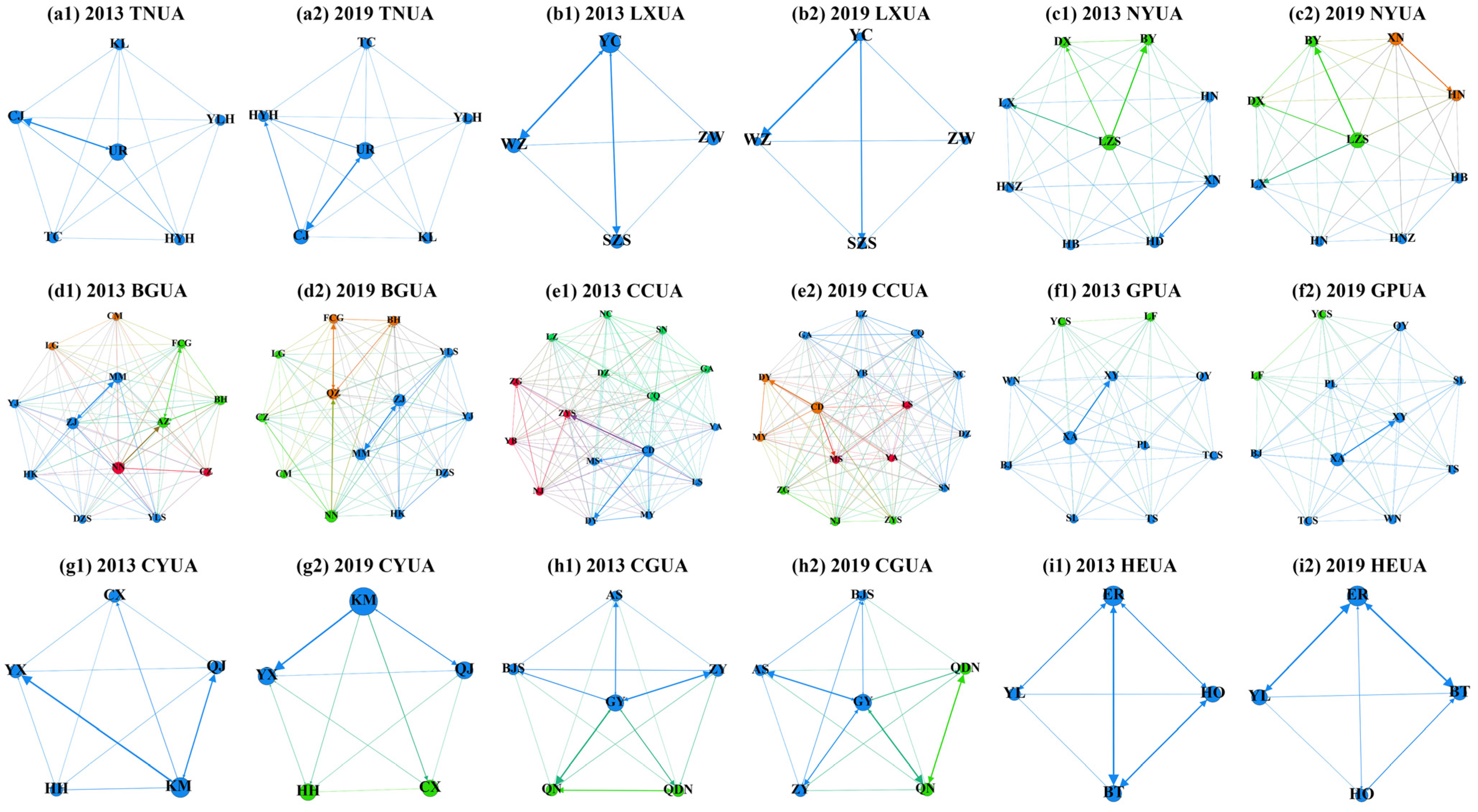
3.4. Economic Connection of Urban Agglomerations

Figure 6 shows the topological network of economic connections between cities in each city cluster in 2013 and 2019. We use different colors to represent the division of cohesive subgroups in the economic network, the size of the nodes to reflect the size of the overall economic connection, and the thickness of the arrows to show the strength of the economic connection.

Overall, between 2013 and 2019, there was significant growth in the economic connection between urban agglomerations. The network of economic connections continued to become deeper and more intricate, which shows that cities are trading more production factors and developing in a more coordinated manner. Geographically, the economic connections between the cities in the center and their neighbors were stronger than those between the cities at the edges of the urban agglomeration. The CCUA has constructed an economic connection network center in Chengdu and Chongqing, the BGUA has constructed a center in Zhanjiang and Nanning, and the GPUA has constructed a center in Xining and Lanzhou. A “double core” spatial network structure is formed by the more complex economic networks of the CCUA, BGUA, and GPUA in particular. In addition, the imbalance of the economic connection between cities is apparent. From the perspective of total economic connection, the exchange of economic elements among cities became closer from 2013 to 2019, and the central cities of each urban agglomeration maintained a much higher total economic connection than other cities. According to the cohesive subgroups of the economic network, each urban agglomeration had a roughly constant number of cohesive subgroups overall, but their composition varied greatly. Cities located closer spatially were more likely to form a cohesive subgroup, indicating a stronger economic connection between them. Particularly, in 2013, the BGUA had four cohesive subgroups, the CCUA had three, and the GPUA, LXUA, and CGUA each had two. The LXUA’s cohesive subgroup number increased to three in 2019, whereas the CYUA’s cohesive subgroup count decreased to two. Based on the above analysis, the increasing economic connection between cities has made the cohesive subgroups of the economic network more rational.

3.5. Network Structural Characteristics of Urban Agglomerations

3.5.1. Network Density of Economic Connection

Table 6. Network density of economic connection networks in 2013 and 2019.

Urban Agglomeration	Network Density in 2013	Network Density in 2019
NYUA	0.22	0.34
GPUA	0.24	0.39
TNUA	0.08	0.11
HEUA	0.21	0.32
CCUA	0.33	0.46
LXUA	0.22	0.38
CYUA	0.25	0.38
CGUA	0.26	0.35
BGUA	0.30	0.40

displays the densities of the economic connectivity network within urban agglomerations. In each urban agglomeration, the density of the economic network significantly increased. However, the overall density of the network was still low, indicating that there is still potential for improvement in the economic connection network structure. The CCUA has the highest network density in 2013 and 2019. The network density was the next highest in the BGUA and GPUA. The TNUA had the lowest density of economic network because of its poor natural environment and limited accessibility. The density of the economic networks within urban agglomerations also exhibited significant imbalances, which is a severe problem requiring attention.

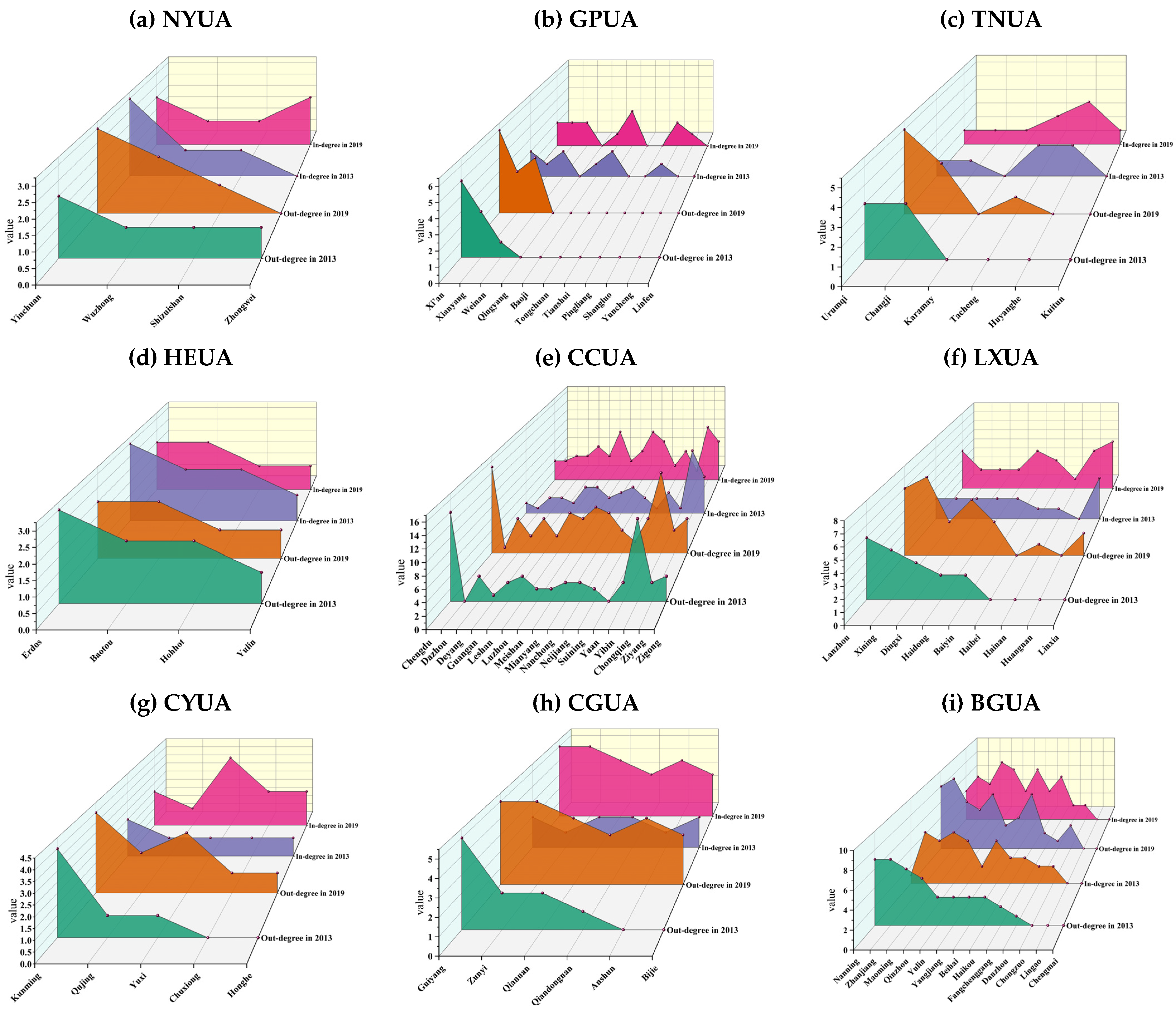
3.5.2. Degree Centrality of Economic Connection

Figure 7 shows the degree centrality of the economic networks within urban agglomerations. In general, there is a significant change in the degree centrality of the cities. Increases in out-degree and in-degree were observed in the central cities. Cities with larger population densities and better geographical locations tended to have higher degree centrality, indicating that they are in the network’s core and have closer connections to nearby cities. Particularly, Chengdu and Chongqing had the highest degree centrality and function as radiating and communicating nodes in the network. Low-degree centrality cities had a restricted potential for economic absorption and radiation and were often located on the periphery of urban agglomerations. To improve the economic network structure and achieve coordinated development, it is essential to improve the quality of cities in peripheral areas and establish an economic connection with core cities.

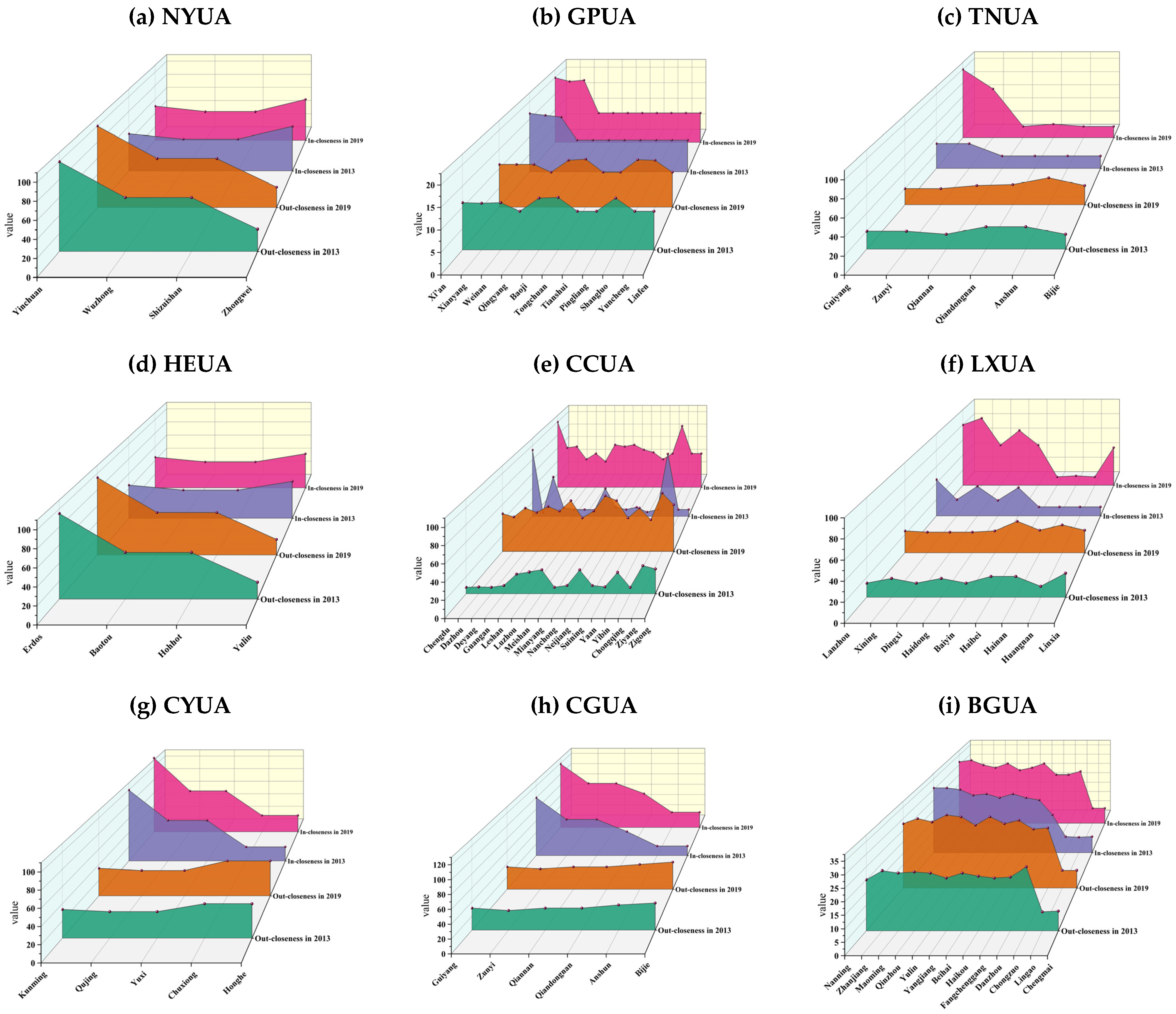
3.5.3. Closeness Centrality of Economic Connection

The closeness centrality of the economic networks within urban agglomerations is shown in Figure 8. Overall, the change in closeness centrality differed between cities, with urban agglomerations including more cities showing a considerable rise. Central cities had higher closeness centrality, whereas cities on the periphery of urban agglomerations had lower closeness centrality. On the one hand, the central cities in urban agglomerations had better economic cooperation and higher closeness centrality in the network. On the other hand, the economic interoperability between cities was weaker in the cities that are located on the periphery of urban agglomerations and have weaker economic independence in growth. Additionally, closeness centrality was clearly out of balance, which was more accentuated in 2019.

3.5.4. Betweenness Centrality of Economic Connection

Table 7. Betweenness centrality of economic connection networks in 2013 and 2019.

Urban Agglomeration	City	Betweenness Centrality		Urban Agglomeration	City	Betweenness Centrality
		2013	2019			2013	2019
CCUA	CD	18.17	33.36	NYUA	UR	0	2.00
	LS	1.33	6.91	GPUA	XA	6	4.50
	LZ	0.83	0		WN	0	0.50
	MS	9.67	47.75	CYUA	KM	6	4.00
	MY	0	2.19		YX	0	7.00
	NC	9.00	28.26	HEUA	ER	2	2.00
	NJ	2.67	26.03		BT	0	2.00
	SN	0	20.19	LXUA	LZ	8.5	15.5
	YB	3.00	3.24		XN	8	7.33
	ZYS	34.50	8.75		DX	0.5	0
	ZG	11.83	5.32		HD	0	2.00
BGUA	NN	2.30	10.45		BY	0	1.83
	ZJ	25.27	14.77		LX	0	1.33
	MM	12.53	2.15	CGUA	GY	9	1.17
	QZ	22.10	12.55		ZY	0	1.17
	YLS	3.50	9.05		QN	4	0.33
	BH	7.80	5.50		AS	0	0.33
	HK	9.50	11.20	NYUA	UR	0	2.00
	FCG	0	0.33

shows the evolution of the betweenness centrality of cities greater than zero. High values of betweenness centrality were concentrated in the central cities of urban agglomerations, which play a core role in the economic network from the perspective of betweenness centrality. A lower betweenness centrality limits cities on the outside of urban agglomerations from functioning as intermediate connections in the economic network. In urban agglomerations with a greater number of cities and a higher overall size, the betweenness centrality is significant. The main reason for this is network complexity, with core node cities playing a part in the transfer of economic resources. Additionally, the disparity in centrality is increasing rapidly. The low betweenness centrality of some cities acts as a barrier to increased economic scale.

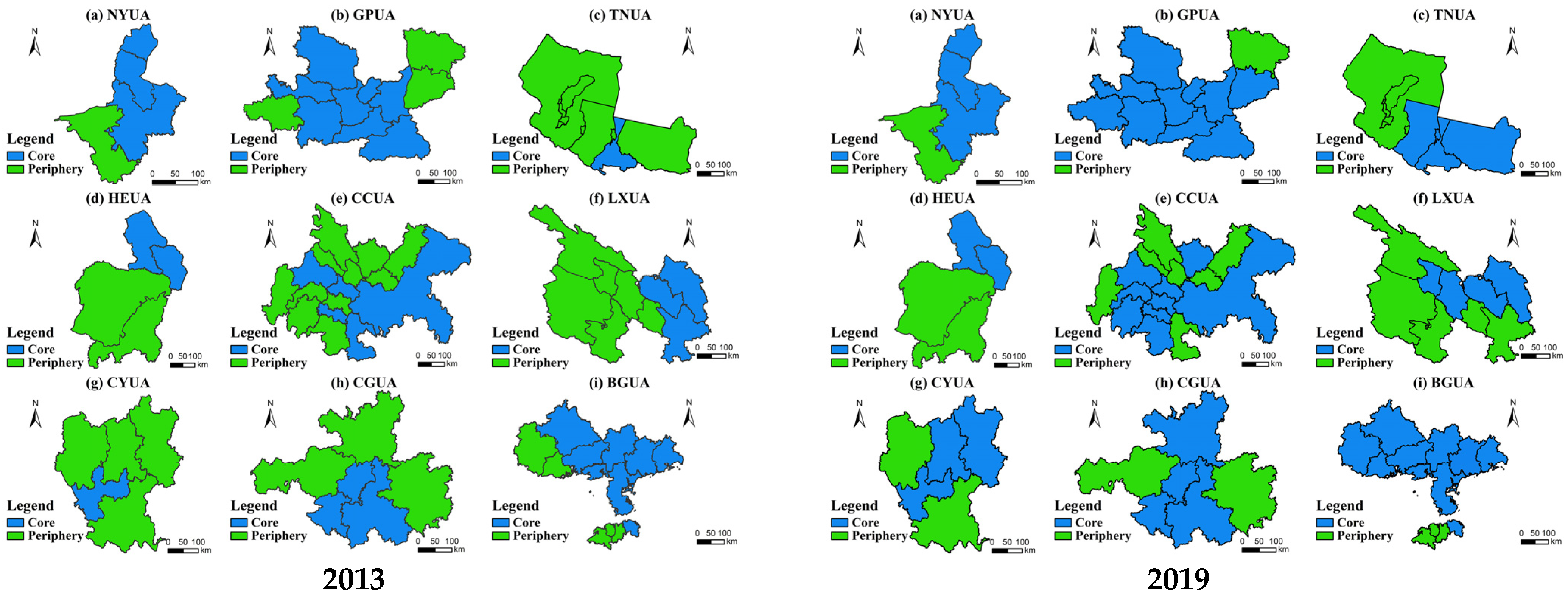
3.5.5. Core–Edge Structure of Economic Connection

The core–edge structure of the economic connection network within each urban agglomeration is shown in Figure 9. The core–edge structures of NYUA and HEUA remained unchanged. On the one hand, there was a single network of economic connections due to the small number of cities. On the other hand, the NYUA and HEUA have few financial resources and weak transportation. A pattern consisting of core area increases and edge area contractions is apparent in the core–edge structures of BGUA, CCUA, CYUA, GPUA, LXUA, CGUA, and TNUA. According to the analysis of the core and edge areas in the networks, the core area is mainly concentrated in cities with a high level of development, convenient transportation, and advantageous location factors. Cities on the periphery of urban agglomerations become the edge areas of the network.

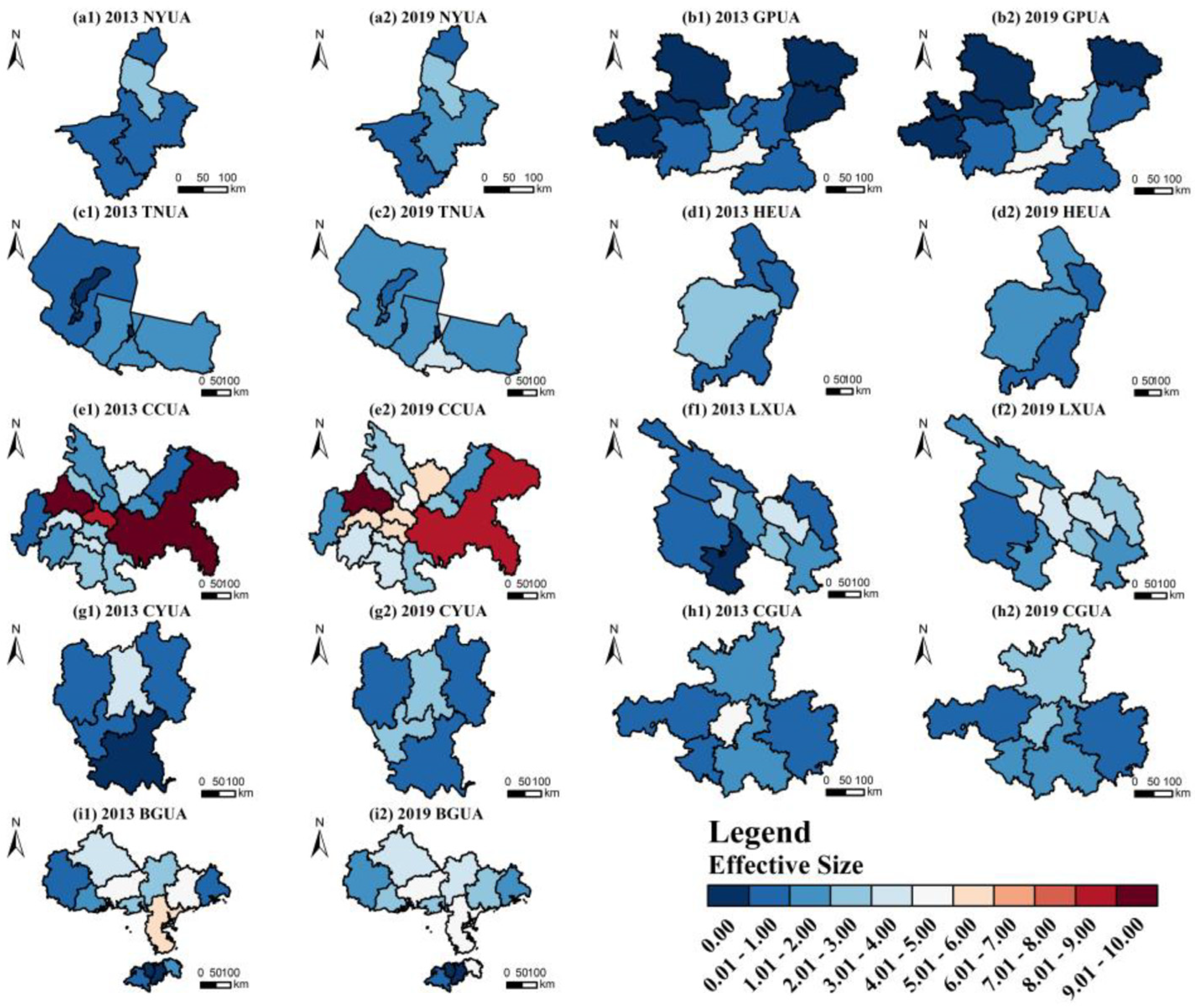
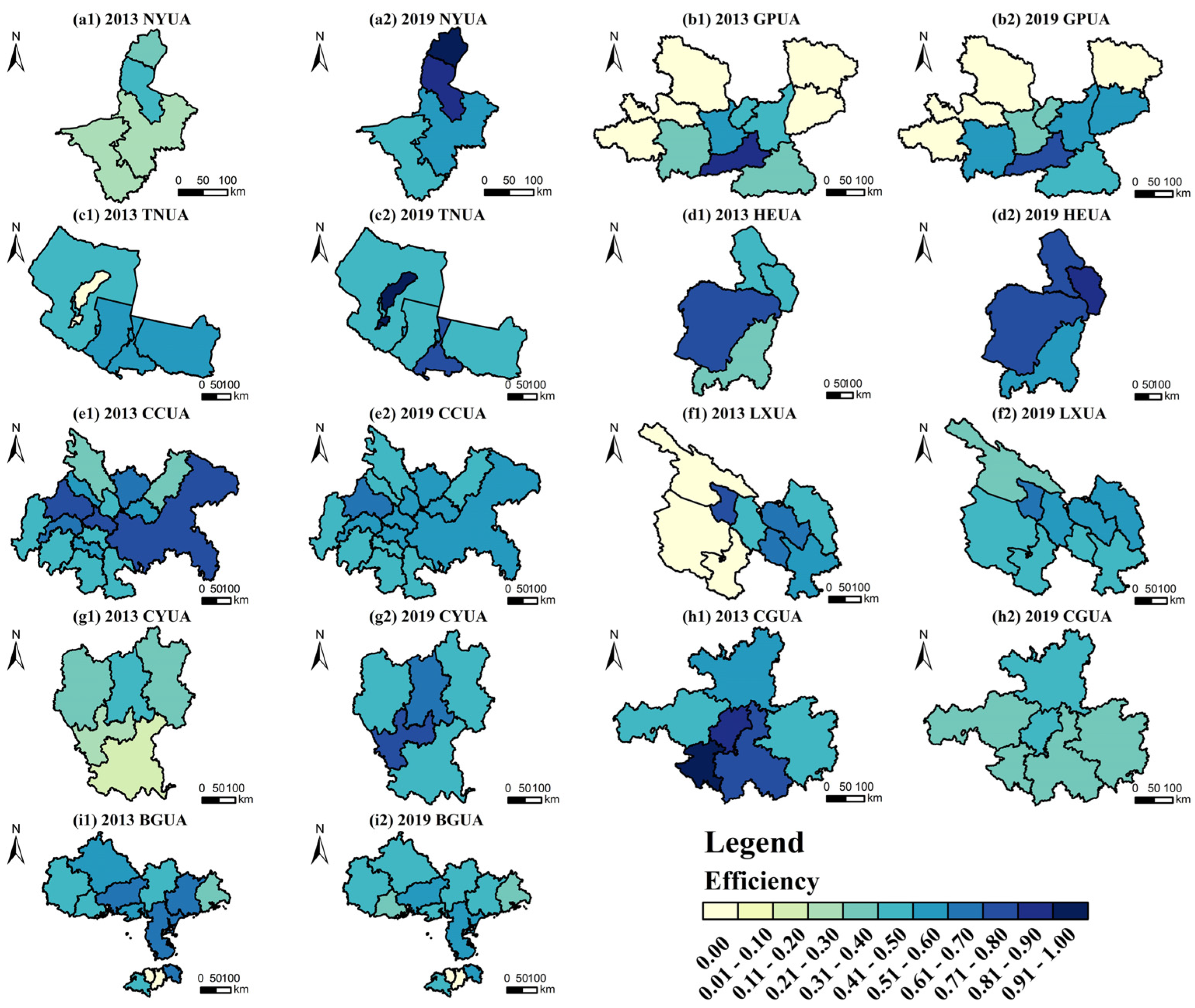
3.5.6. Structural Hole of Economic Connection

We calculated the effective size of the economic connection network by applying structural hole analysis (Figure 10). Each city’s actual size experienced a significant increase. The high values of effective size were concentrated in the center cities, which have greater power and control over other cities and are located near the network’s core. This supports the prominence of central cities in the economic network. Low effective size values were primarily observed near the periphery of urban agglomerations. This is mostly caused by the low economic development of peripheral cities, which frequently keeps them outside of the periphery of the economic network. The highest effective size in the CCUA were observed for Chengdu and Chongqing, indicating that they have an advantage of more apparent structural holes in the economic network.

Figure 11 shows the efficiency of the economic connection networks within urban agglomerations. A structural hole is a sign of increased efficiency, individuals acting more effectively and having more of an influence on other network members. Central cities in urban agglomerations, which have a higher ability to influence and control neighboring cities, are concentrated in high efficiency; for instance, Zhanjiang and Nanning in the BGUA, Chengdu, Chongqing in the CCUA, and Xi’an in the GPUA. They have highly efficiency due to their geographic position, resource availability, and other benefits. Additionally, during the study period, Tianshui, Qingyang, Linfen, and Pingliang’s efficiency in the GPUA was always 0. This is primarily owing to their limited economic scale and inability to effectively influence and control the cities around them.

3.6. Economic Connections between Urban Agglomerations

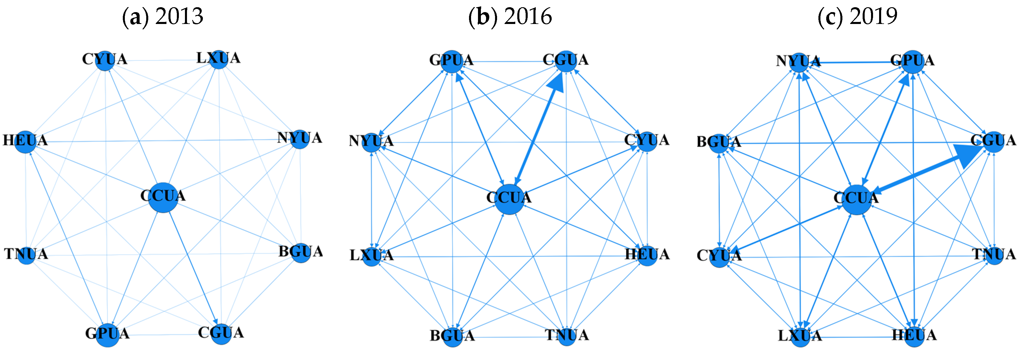
3.6.1. Evolution of Economic Connection

The topological network of economic connections between urban agglomerations in the NWLSC is shown in Figure 12. It is apparent that during the study period, networks became more complex and the economic connections between urban agglomerations strengthened. The economic connection network in 2019 showed hierarchical characteristics. The CCUA, CGUA, CYUA, and GPUA form a high-level economic connection network, and the LXUA, NYUA, HEUA, TNUA, and BGUA form a mid-level economic connection network. The CCUA develops into a core node of the geographical network of economic connectedness, forming a radial spatial network with the nearby urban agglomerations. Additionally, the economic connection imbalance increased, indicating that center urban agglomerations have a far stronger economic connection than periphery urban agglomerations. Due to the spatial distance between peripheral urban agglomerations and others being greater, rising transportation costs impede the movement of production elements between urban agglomerations to some extent.

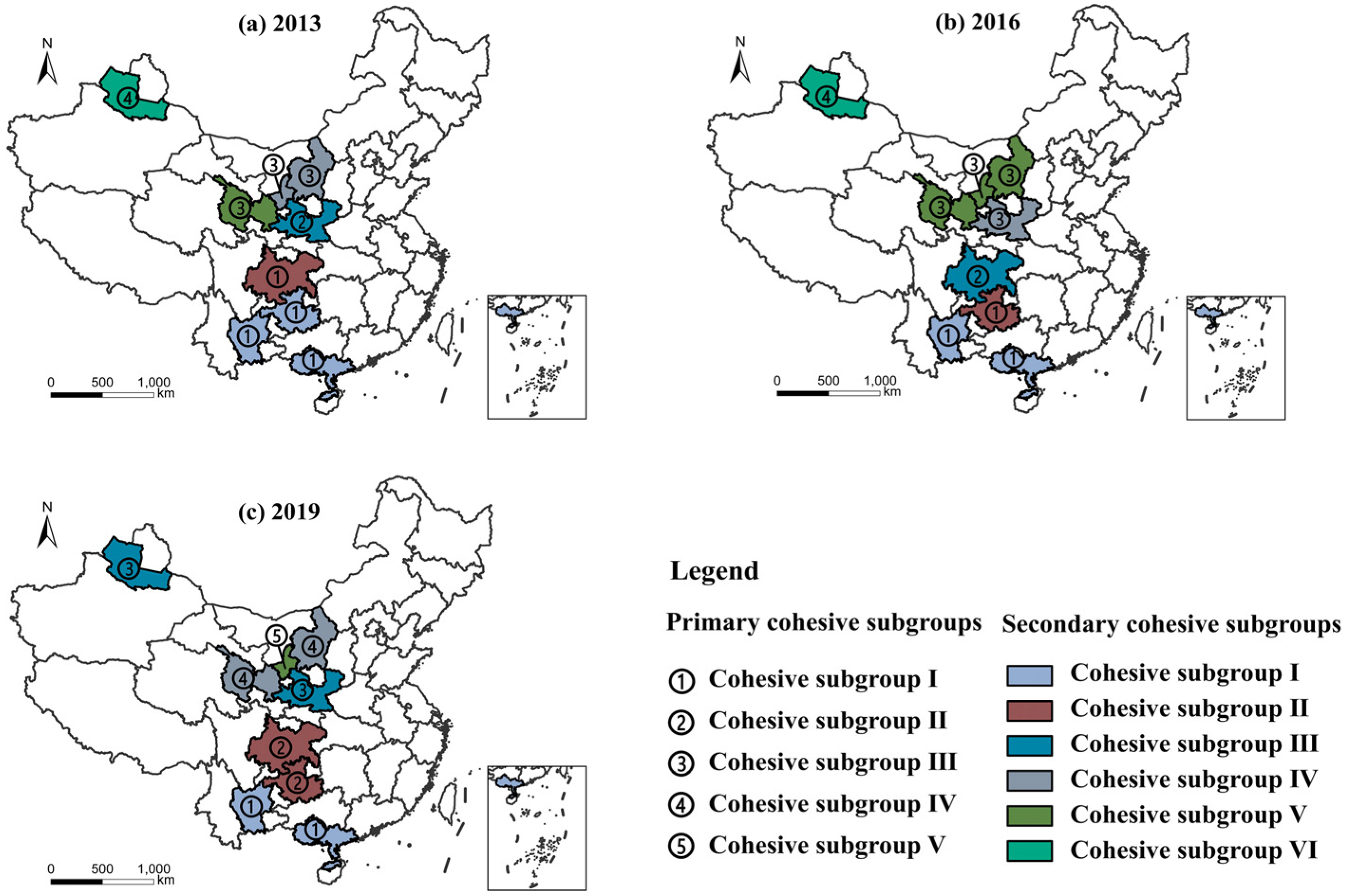
3.6.2. Cohesive Subgroups of the Economic Connection

Figure 13 shows the cohesive subgroups of the economic connection network between urban agglomerations. During the study period, urban agglomerations exhibited a clear agglomeration phenomenon and exhibited particular geographic proximity characteristics in the NWLSC. The number of primary and secondary cohesive subgroups remained relatively constant, but the internal member makeup shifted dramatically. From the division of primary cohesive subgroups, five larger cohesive subgroups were generated in 2013 and 2016, and six larger cohesive subgroups were formed in 2019. To form new regional groups, single cohesive subgroups gradually mix with other cohesive subgroups. Larger subgroups are divided into smaller subgroups. From the division of secondary cohesive subgroups, the number of subgroups decreased from six in 2013 and 2016 to five in 2019. There were far fewer single subgroups, resulting in the formation of regional group subgroups. The CCUA and the CGUA, for example, are geographically close, have greater economic connection, and have more regular inter-regional economic interactions, making it easier to form a subgroup. The network density of secondary cohesive subgroups indicates an overall increase. Additionally, the network density of agglomerative subgroups was uneven.

Table 8. Network density of secondary cohesive subgroups in 2013, 2016, and 2019.

Year	2013						2016						2019
cohesive subgroups	I	II	III	IV	V	VI	I	II	III	IV	V	VI	I	II	III	IV	V
I	0	0	1	0	1	1	0	1	1	0	1	0.67	0.5	1	0	0	0
II	0	0.33	1	0	0	0	1	0	1	0	0	0	1	1	0.25	0.5	0
III	1	1	0	0	0	1	1	1	0	0	0	0	0	0.5	0	0.5	0.5
IV	0	0	0	0	0	0	0	0	0	0	0	0	0	0	0.25	0	0
V	0	0	0	0	0	0	1	0	0	0	0	1	0	0	0	0	0
VI	0	0	0	0	0	0	0	0	0	0	0.33	0	\	\	\	\	\

shows that the network density of cohesive subgroups was usually 1, whereas the density of other subgroups was 0.

3.7. Network Structural Effect of Urban Agglomerations

3.7.1. Overall Network Structure Effect

Taking the mean value of t economic connection strength between urban agglomerations as the explained variable and network density, network efficiency, and network hierarchy as the explanatory variable, we used regression analysis to evaluate the effect of network structure (

Table 9. Regression analysis of the overall network.

Explained Variable	Mean Value of Economic Connection Strength
Model	(1)	(2)	(3)
Constants	−0.046	1.011 **	0.660
	(0.091)	(0.053)	(0.340)
Network density	1.009 *
	(0.144)
Network efficiency		−0.979 **
		(0.074)
Network hierarchy			−0.660
			(0.589)
R2	0.980	0.994	0.556

Note: The values in parentheses in the table are standard errors, and *, and ** represent the significance levels of 10%, and 5%, respectively.

). In contrast to the network density coefficient, which was found to be significant at the 10% level, the network efficiency coefficient was demonstrated to be significant at the 5% level. The network density and efficiency have great fitting effects, and the R² values are both higher than 0.98.

The network density and network efficiency regression coefficients are 1.009 and −0.979, respectively, showing that network density and efficiency can strengthen the economic connections between urban agglomerations in the NWLSC by increasing network density and decreasing network efficiency. First, the higher network density reflects increased economic connections between urban agglomerations. The development of urban agglomerations at the periphery is supported by those in the economic network’s core, which enhances interurban economic cooperation. Second, as network efficiency declines, more connections become functional, which considerably improves the economic connection between urban agglomerations.

3.7.2. Individual Network Structure Effect

We used the economic connection strength of each urban agglomeration in the NWLSC as the explained variable, and explanatory variables such as degree centrality, closeness centrality, betweenness centrality, effective scale, and structural hole efficiency to build a panel model for regression analysis (

Table 10. Regression analysis of the individual networks.

Model	(1)	(2)	(3)	(4)	(5)
Constants	−0.034	−0.085	0.114 **	0.102	0.503 ***
	(0.068)	(0.088)	(0.041)	(0.116)	(0.137)
Degree centrality	0.509 ***
	(0.134)
Closeness centrality		0.483 ***
		(0.139)
Betweenness centrality			0.441 **
			(0.159)
Effective scale				0.330
				(0.326)
Efficiency					−0.441 *
					(0.211)
R2	0.460	0.416	0.310	0.057	0.205

Note: The values in parentheses in the table are standard errors, and *, **, and *** represent the significance levels of 10%, 5%, and 1%, respectively.

). Models (1) and (2) pass the 1% significance level test, Model (3) passes the 5% significance level test, and Model (4) passes the 10% significance level test.

The economic connection between urban agglomerations increases by 0.509% for every 1% rise in each node’s degree centrality, as shown in Table 9. The regression coefficient of closeness centrality is 0.483, indicating that an increase in closeness centrality encourages the circulation of production factors and cooperation between urban agglomerations. With the betweenness centrality regression value of 0.441, it can be seen that urban agglomerations with high betweenness centrality have clear comparative advantages in the network and successfully obtain transfer share from others. The structural hole’s efficiency has a regression coefficient of −0.441, indicating that decreasing efficiency can improve the economic connections between urban agglomerations. To successfully reduce the imbalance of economic connections and enhance network node efficiency, the government should take measures to significantly increase economic dependence between urban agglomerations.

4. Discussion

Figure 3, Figure 4 and Figure 5 show how the spatial direction, spatial heterogeneity, and local dynamics evolution of urban agglomerations’ economic development in the NWLSC changed dramatically. The dynamically changing and interacting processes of economic development between neighboring cities are more obvious. To promote the development of China’s western cities in terms of policies, resources, and funding, the Chinese government has implemented regional development strategies, such as the development of western regions in the new era. The advantages of economic scale and resource availability are present in the core city, and the value of NTL is high. Because of its excellent geographic location, developed transportation, and reasonable industrial division, the CCUA is a key force for economic development in the western part of China. The BGUA is situated near the Pearl River Delta, one of China’s most prosperous regions, and at the beginning of the Maritime Silk Road. As a result, the economic growth of CCUA and BGUA has altered considerably throughout time and has spread to neighboring cities. In the northwest of China, where resources are few and transportation is undeveloped, are the TNUA, GPUA, and LXUA. The economic space of the urban agglomerations has been steadily contracting as a result of the concentration of economic resources in the center cities. Therefore, the development of urban agglomerations should promote the radiation effect of large cities, while reducing the gap between urban development in the future.

It is clear from Figure 6 and Figure 12 that urban agglomerations in the NWLSC are becoming more economically connected over time, eventually forming an economic network. Technology, transportation, and logistics advancements contribute to the development of resource components across cities. While the peripheral cities have poor economic cooperation and connection with other cities due to geography, the center cities of urban clusters, such as Chengdu, Chongqing, and Nanning, promote the development of adjacent cities in the economic network. Urban agglomeration growth is limited by the unbalanced economic connections across cities. The CCUA is located in the geographic center of the NWLSC, and because of its high rate of innovation, large labor pool, and well-developed transportation system, it has established its position at the center of the economic network. The NYUA’s weak economic base and remote location from other urban agglomerations make it difficult for production factors to flow freely.

The spatial resolutions and accuracy of NTL data influence the accuracy of the economic connection structure developed in this study. There are some limitations with NTL data such as coarse spatial and radiometric resolutions [72,73]. Because of sensor defects and other factors, NTL data such as DMSP-OLS remote sensing images have problems with overflow and saturation effects [40]. In addition, there are errors in the observation, transmission, and processing of NTL data, which impact the results of the study. The NTL images are limited in monitoring human activities in unlighted areas and have weak predictive performance for microscopic spatial units [74]. In addition, urban agglomerations are also well-organized and structured economic entities. The formation of urban agglomerations is encouraged by specialization of production and distinct divisions of industries. Technology, institutions, policies, culture, and industrial structure vary between urban agglomerations. Economic growth and connectivity are substantially influenced by the different functional zoning of cities.

In the next study, we will focus on the following aspects. Firstly, we will integrate NTL data with higher spatial resolution and spatial big data such as population migration data, social media data, traffic network data, and point of interest data to investigate the economic development of urban agglomerations. The modifiable areal unit problem in different spatial scales and functional districts will also be considered. Secondly, the relationship between NTL aggregation characteristics and urban functional districts at the pixel level will be analyzed, which will help us to examine changes in the economic connections between micro-administrative units including counties and suburbs using spatial big data. Finally, it is worth studying how administrative zoning and economic scope affect the spatial structure of the economic connection network, which is an important factor in future urban agglomeration development planning.

5. Conclusions and Recommendations

5.1. Conclusions

This study focuses on the economic connections between urban agglomerations in the NWLSC. We analyzed the spatial dynamics, spatial trends, and spatial agglomeration of urban agglomeration economic development patterns. The structural characteristics of the economic network and key influencing factors were investigated using the SNA approach. The primary conclusions reached are as follows.

The economic size of urban agglomerations in the NWLSC grew from 2013 to 2019. The economic gravity center of urban agglomerations moved dramatically, and the spatial structure displayed diverse characteristics. The CCUA and BGUA economic structures showed a feature known as “double-core concentration”, which promotes the development of the surrounding cities.

The economic connections within and between urban agglomerations increased dramatically. The network of economic connections deepened and a multi-level network started to emerge. The CCUA gradually developed into the core of the economic network in the NWSLC because of its advantageous geographic location and significant economic volume. Additionally, the imbalance of economic connection gradually increased, with cities in the center of urban agglomerations having high value and weak economic connection to the periphery cities.

Considering the spatial structure of the economic network, the urban agglomeration network density greatly increased. The center cities became the core of the economic networks with strong control and intermediation capabilities. There was a clear tendency for urban agglomerations to cluster, and the economic connection became closer. However, the economic absorption and radiation capacity in the economic network need to be further improved in cities that are at the edges of urban agglomerations.

According to the results of the network structural effect, the increased network density and centrality encourage economic connection between urban agglomerations, but network efficiency restricts the movement of economic forces. The higher the efficiency of structural holes, the greater effect on other individuals, which reduces the intensity of dependence and cooperation between urban agglomerations.

5.2. Recommendations

Based on the important findings of this study and the current economic and social development in the NWLSC, we put forward policy recommendations to promote economic coordination and high-quality development.

First, the geographical environment, economic development, and resource assets of the NWLSC are all heterogeneous. To reduce the space-time distance for resource element movement, the government should accelerate the development of infrastructure including trains and highways as well as the connection of inter-city transportation networks. The above measures improve the effectiveness of economic connection by optimizing the network structure of economic connection.

Second, the core cities of the network play a significant role in spatial radiation. It is critical to raise the comprehensive level of core cities to fully exploit their leadership potential. Increased financial and policy support for cities located on the periphery of urban agglomerations, which can promote coordinated economic development. It is necessary to build multi-level regional economic development growth poles with major, medium, and small cities and develop the radiation capacity of cities in the local economic network.

Third, constructing a management platform for coordinated regional development to increase the mechanisms for symbiotic development, which can encourage production factors to move more freely. Cities must improve economic cooperation and communication to achieve better coordinated economic development. The government should clarify the division of functions among cities and adopt regional development plans based on local conditions. Furthermore, establishing a regional economic coordinated development framework is critical for realizing the complementing benefits of resource elements.

References

1. Liu, Y.; Zhang, X.; Pan, X.; Ma, X.; Tang, M. The spatial integration and coordinated industrial development of urban agglomerations in the Yangtze River Economic Belt, China. Cities 2020, 104, 102801. [Google Scholar] [CrossRef]
2. Qin, X.; Qian, Y.; Zeng, J.; Wei, X. Accessibility and economic connections between cities of the new western land–sea corridor in china—enlightenments to the passageway strategy of gansu province. Sustainability 2022, 14, 4445. [Google Scholar] [CrossRef]
3. Chen, H.; Dong, Q. The spatial difference and impact effect of urban innovation at the new Western Land–Sea corridor. J. Chongqing Univ. Technol. (Soc. Sci.) 2021, 35, 58–67. [Google Scholar]
4. Matthieu, C.; Pamina, K. Structural gravity equations with intensive and extensive margins. Can. J. Econ. 2010, 43, 41–62. [Google Scholar]
5. Zipf, G.K. The PIP2/D hypothesis: On the Intercity movement of persons. Am. Sociol. Rev. 1946, 11, 677–686. [Google Scholar] [CrossRef]
6. Xie, W.; Li, H.; Yin, Y. Research on the Spatial Structure of the European Union’s Tourism Economy and Its Effects. Int. J. Environ. Res. Public Health 2021, 18, 1389. [Google Scholar] [CrossRef]
7. Chen, X.; Wang, T.; Zheng, X.; Han, F.; Yang, Z. The structure and evolution of the tourism economic network of the Tibetan Plateau and its driving factors. Land 2022, 11, 241. [Google Scholar] [CrossRef]
8. Huang, Y.; Hong, T.; Ma, T. Urban network externalities, agglomeration economies and urban economic growth. Cities 2020, 107, 102882. [Google Scholar] [CrossRef]
9. Wang, K.; Wang, M.; Gan, C.; Chen, Q.; Voda, M. Tourism economic network structural characteristics of national parks in the central region of China. Sustainability 2021, 13, 4805. [Google Scholar] [CrossRef]
10. Wang, F.; Chai, W.; Shi, X.; Dong, M.; Yan, B. Does regional financial resource contribute to economic growth? From the perspective of spatial correlation network. SAGE Open 2021, 11. [Google Scholar] [CrossRef]
11. Ye, S.; Qian, Z. The economic network resilience of the Guanzhong Plain City Cluster, China: A network analysis from the evolutionary perspective. Growth Change 2021, 52, 2391–2411. [Google Scholar] [CrossRef]
12. Jin, R.; Gong, J.; Deng, M.; Wan, Y.; Yang, X. A framework for spatiotemporal analysis of regional economic agglomeration patterns. Sustainability 2018, 10, 2800. [Google Scholar] [CrossRef]
13. Zhao, X.; Su, J.; Chao, J.; Liu, X.; Li, T.; Rui, Y.; Yang, J. The character and economic preference of city network of china: A study based on the Chinese global fortune 500 enterprises. Complexity 2020, 2020, 4312578. [Google Scholar] [CrossRef]
14. Zheng, Y.; Lu, M.; Li, J. Internal circulation in China: Analyzing market segmentation and integration using big data for truck traffic flow. Econ. Model. 2022, 115, 105975. [Google Scholar] [CrossRef]
15. Zhu, Z.; Wang, L.; Liu, W.; Qi, D. Relationship between urban economic connections and geoeconomic relations in northeast China. Complexity 2020, 2020, 5263048. [Google Scholar] [CrossRef]
16. Yu, G.; He, D.; Lin, W.; Wu, Q.; Xiao, J.; Lei, X.; Xie, Z.; Wu, R.; Jaramillo, S.M. China’s spatial economic network and its influencing factors. Complexity 2020, 2020, 6352021. [Google Scholar] [CrossRef]
17. Chen, Y.; Jiang, A. Spatial characteristics and complexity of the urban economic network structure based on the secure internet of things. Sustain. Comput. Inf. Syst. 2022, 35, 100729. [Google Scholar] [CrossRef]
18. Wang, H.; Kilmartin, L. Comparing rural and urban social and economic behavior in Uganda: Insights from mobile voice service usage. J. Urban Technol. 2014, 21, 61–89. [Google Scholar] [CrossRef]
19. Chu, N.; Zhang, P.; Li, H. Transnational economic connection analysis based on railway class accessibility between China and Russia. Chin. Geogr. Sci. 2019, 29, 872–886. [Google Scholar] [CrossRef] [Green Version]
20. Li, M.; Guo, W.; Guo, R.; He, B.; Li, Z.; Li, X.; Liu, W.; Fan, Y. Urban network spatial connection and structure in China based on railway passenger flow big data. Land 2022, 11, 225. [Google Scholar] [CrossRef]
21. Jiang, J.; Chen, J.; Tu, W.; Wang, C. A Novel effective indicator of weighted inter-city human mobility networks to estimate economic development. Sustainability 2019, 11, 6348. [Google Scholar] [CrossRef] [Green Version]
22. Hu, S.; Yang, H.; Cai, B.; Yang, C. Research on spatial economic structure for different economic sectors from a perspective of a complex network. Phys. A 2013, 392, 3682–3697. [Google Scholar] [CrossRef]
23. Sylvain, D. The role of distance and social networks in the geography of crowdfunding: Evidence from France. Reg. Stud. 2019, 54, 329–339. [Google Scholar]
24. Gan, C.; Voda, M.; Wang, K.; Chen, L.; Ye, J. Spatial network structure of the tourism economy in urban agglomeration: A social network analysis. J. Hosp. Tour. Manag. 2021, 47, 124–133. [Google Scholar] [CrossRef]
25. Feng, R.; Wang, K. Spatiotemporal evolution of the constraint strength of “administrative regional economy” from the perspective of regional economic integration: A case study of the Chengdu-Deyang-Mianyang region, China. Prog. Geogr. 2020, 39, 1447–1459. (In Chinese) [Google Scholar] [CrossRef]
26. Wu, S.; Zhong, Y.; Wu, Q.; Mao, W. Multi-outward connection networks of urban agglomeration: An empirical study from middle reaches of yangtze river to yangtze river economic belt. Resour. Environ. Yangtze Basin 2021, 30, 2360–2372. (In Chinese) [Google Scholar]
27. Kim, A.C.H.; Newman, J.I.; Kwon, W. Developing community structure on the sidelines: A social network analysis of youth sport league parents. Soc. Sci. J. 2020, 57, 178–194. [Google Scholar] [CrossRef]
28. Jinliao, H.; Xianpeng, W.; Gang, Z. Creative city networks: A social network analysis of a virtual community of designers in China. Cities 2022, 123, 103578. [Google Scholar] [CrossRef]
29. Lu, W.; Park, S.H.; Liu, S.; Nam, T.H.; Yeo, G.T. Connection analysis of container ports of the bohai rim economic circle (BREC). Asian J. Shipping Log. 2018, 34, 145–150. [Google Scholar] [CrossRef]
30. Guo, Y.; Cao, L.; Song, Y.; Wang, Y.; Li, Y. Understanding the formation of City-HSR network: A case study of Yangtze River Delta, China. Transp. Policy 2022, 116, 315–326. [Google Scholar] [CrossRef]
31. Huang, X.; Li, G.; Song, Y.; Liu, J. The impact of spatial structure on economic efficiency of Beijing-Tianjin-Hebei megalopolis in China. Complexity 2020, 2020, 6038270. [Google Scholar] [CrossRef]
32. Sun, Q.; Tang, F.; Tang, Y. An economic tie network-structure analysis of urban agglomeration in the middle reaches of Changjiang River based on SNA. J. Geogr. Sci. 2015, 25, 739–755. [Google Scholar] [CrossRef] [Green Version]
33. Croft, T.A. Nighttime images of the earth from space. Sci. Am. 1978, 239, 86–101. [Google Scholar] [CrossRef]
34. Ch, R.; Martin, D.A.; Vargas, J.F. Measuring the size and growth of cities using nighttime light. J. Urban. Econ. 2021, 125, 103254. [Google Scholar] [CrossRef]
35. Yu, M.; Guo, S.; Guan, Y.; Cai, D.; Zhang, C.; Fraedrich, K.; Liao, Z.; Zhang, X.; Tian, Z. Spatiotemporal heterogeneity analysis of Yangtze River Delta urban agglomeration: Evidence from nighttime light data (2001–2019). Remote Sens. 2021, 13, 1235. [Google Scholar] [CrossRef]
36. Fu, H.; Shao, Z.; Fu, P.; Cheng, Q. The dynamic analysis between urban nighttime economy and urbanization using the DMSP/OLS nighttime light data in china from 1992 to 2012. Remote Sens. 2017, 9, 416. [Google Scholar] [CrossRef] [Green Version]
37. Keola, S.; Andersson, M.; Hall, O. Monitoring economic development from space: Using nighttime light and land cover data to measure economic growth. World Dev. 2015, 66, 322–334. [Google Scholar] [CrossRef]
38. Liu, S.; Shi, K.; Wu, Y.; Chang, Z. Remotely sensed nighttime lights reveal China’s urbanization process restricted by haze pollution. Transp. Policy 2021, 206, 108350. [Google Scholar] [CrossRef]
39. Alahmadi, M.; Atkinson, P.M. Three-fold urban expansion in Saudi Arabia from 1992 to 2013 observed using calibrated DMSP-OLS night-time lights imagery. Remote Sens. 2019, 11, 2266. [Google Scholar] [CrossRef] [Green Version]
40. Alahmadi, M.; Mansour, S.; Martin, D.; Atkinson, P.M. An improved index for urban population distribution mapping based on nighttime lights (DMSP-OLS) data: An experiment in Riyadh Province, Saudi Arabia. Remote Sens. 2021, 13, 1171. [Google Scholar] [CrossRef]
41. Chen, X.; Nordhaus, W.D. VIIRS nighttime lights in the estimation of cross-sectional and time-series GDP. Remote Sens. 2019, 11, 1057. [Google Scholar] [CrossRef] [Green Version]
42. Yin, J.; Qiu, Y.; Zhang, B. Identification of poverty areas by remote sensing and machine learning: A case study in Guizhou, Southwest China. ISPRS Int. J. Geo-Inf. 2020, 10, 11. [Google Scholar] [CrossRef]
43. Weidmann, N.B.; Theunissen, G. Estimating local inequality from nighttime lights. Remote Sens. 2021, 13, 4624. [Google Scholar] [CrossRef]
44. Chen, Z.; Wei, Y.; Shi, K.; Zhao, Z.; Wang, C.; Wu, B.; Qiu, B.; Yu, B. The potential of nighttime light remote sensing data to evaluate the development of digital economy: A case study of China at the city level. Comput. Environ. Urban Syst. 2022, 92, 101749. [Google Scholar] [CrossRef]
45. Cui, Y.; Shi, K.; Jiang, L.; Qiu, L.; Wu, S. Identifying and evaluating the nighttime economy in China using multisource data. IEEE Geosci. Remote Sens. Lett. 2021, 18, 1906–1910. [Google Scholar] [CrossRef]
46. Chen, Z.; Yu, B.; Yang, C.; Zhou, Y.; Yao, S.; Qian, X.; Wang, C.; Wu, B.; Wu, J. An extended time series (2000–2018) of global NPP-VIIRS-like nighttime light data from a cross-sensor calibration. Earth Sys. Sci. Data 2021, 13, 889–906. [Google Scholar] [CrossRef]
47. Li, Y.; Ye, H.; Gao, X.; Sun, D.; Li, Z.; Zhang, N.; Leng, X.; Meng, D.; Zheng, J. Spatiotemporal Patterns of urbanization in the three most developed urban agglomerations in China based on continuous nighttime light data (2000–2018). Remote Sens. 2021, 13, 2245. [Google Scholar] [CrossRef]
48. Gibson, J.; Boe-Gibson, J. Nighttime Lights and County-Level Economic Activity in the United States: 2001 to 2019. Remote Sens. 2021, 13, 2741. [Google Scholar] [CrossRef]
49. Li, X.; Xu, H.; Chen, X.; Li, C. Potential of NPP-VIIRS nighttime light imagery for modeling the regional economy of China. Remote Sens. 2013, 5, 3057–3081. [Google Scholar] [CrossRef] [Green Version]
50. Zhang, Q.; Seto, K.C. Mapping urbanization dynamics at regional and global scales using multi-temporal DMSP/OLS nighttime light data. Remote Sens. Environ. 2011, 115, 2320–2329. [Google Scholar] [CrossRef]
51. Li, Y.; Zuo, Z.; Xu, D.; Wei, Y. Mining eco-efficiency measurement and driving factors identification based on Meta-US-SBM in Guangxi Province, China. Int. J. Environ. Res. Public Health 2021, 18, 5397. [Google Scholar] [CrossRef] [PubMed]
52. Qiu, Y.; Yin, J.; Zhang, T.; Du, Y.; Zhang, B. Spatiotemporal dynamic analysis of a-level scenic spots in Guizhou Province, China. ISPRS Int. J. Geo-Inf. 2021, 10, 568. [Google Scholar] [CrossRef]
53. Aghadadashi, V.; Molaei, S.; Mehdinia, A.; Mohammadi, J.; Moeinaddini, M.; Riyahi Bakhtiari, A. Using GIS, geostatistics and Fuzzy logic to study spatial structure of sedimentary total PAHs and potential eco-risks; An Eastern Persian Gulf case study. Mar. Pollut. Bull. 2019, 149, 110489. [Google Scholar] [CrossRef] [PubMed]
54. Rey, S.J.; Murray, A.T.; Anselin, L. Visualizing regional income distribution dynamics. Lett. Spat. Resour. Sci. 2011, 4, 81–90. [Google Scholar] [CrossRef]
55. Zhang, B.; Yin, J.; Jiang, H.; Qiu, Y. Spatial–temporal pattern evolution and influencing factors of coupled coordination between carbon emission and economic development along the Pearl River Basin in China. Environ. Sci. Pollut. Res. 2022. [Google Scholar] [CrossRef]
56. Ye, X.; Rey, S. A framework for exploratory space-time analysis of economic data. Ann. Regional Sci. 2011, 50, 315–339. [Google Scholar] [CrossRef]
57. Jiang, H.; Yin, J.; Qiu, Y.; Zhang, B.; Ding, Y.; Xia, R. Industrial carbon emission efficiency of cities in the pearl river basin: Spatiotemporal dynamics and driving forces. Land 2022, 11, 1129. [Google Scholar] [CrossRef]
58. Pei, Z.; Han, G.; Ma, X.; Shi, T.; Gong, W. A Method for estimating the background column concentration of CO2 using the lagrangian. IEEE Trans. Geosci. Remote Sens. 2022, 60, 4108112. [Google Scholar] [CrossRef]
59. Fan, Y.; Zhang, S.; He, Z.; He, B.; Yu, H.; Ye, X.; Yang, H.; Zhang, X.; Chi, Z. Spatial pattern and evolution of urban system based on gravity model and whole network analysis in the huaihe river basin of China. Discrete Dyn. Nat. Soc. 2018, 2018, 3698071. [Google Scholar] [CrossRef]
60. Liu, Z.; Mu, R.; Hu, S.; Li, M.; Wang, L. The method and application of graphic recognition of the social network structure of urban agglomeration. Wirel. Pers. Commun. 2018, 103, 447–480. [Google Scholar] [CrossRef]
61. Li, X.; Lu, Y.; Huang, R. Whether foreign direct investment can promote high-quality economic development under environmental regulation: Evidence from the Yangtze River Economic Belt, China. Environ. Sci. Pollut. Res. 2021, 28, 21674–21683. [Google Scholar] [CrossRef] [PubMed]
62. Kong, Q.; Peng, D.; Ni, Y.; Jiang, X.; Wang, Z. Trade openness and economic growth quality of China: Empirical analysis using ARDL model. Financ. Res. Lett. 2021, 38, 101488. [Google Scholar] [CrossRef]
63. Peng, B.; Sheng, X.; Wei, G. Does environmental protection promote economic development? From the perspective of coupling coordination between environmental protection and economic development. Environ. Sci. Pollut. Res. 2020, 27, 39135–39148. [Google Scholar] [CrossRef] [PubMed]
64. Esteves, R.; Geisler Mesevage, G. Social networks in economic history: Opportunities and challenges. Explor. Econ. Hist. 2019, 74, 101299. [Google Scholar]
65. Bai, C.; Zhou, L.; Xia, M.; Feng, C. Analysis of the spatial association network structure of China’s transportation carbon emissions and its driving factors. J. Environ. Manag. 2020, 253, 109765. [Google Scholar] [CrossRef] [PubMed]
66. Lovrić, M.; Da Re, R.; Vidale, E.; Pettenella, D.; Mavsar, R. Social network analysis as a tool for the analysis of international trade of wood and non-wood forest products. For. Policy Econ. 2018, 86, 45–66. [Google Scholar] [CrossRef]
67. Song, J.; Feng, Q.; Wang, X.; Fu, H.; Jiang, W.; Chen, B. Spatial association and effect evaluation of CO2 emission in the Chengdu-Chongqing urban agglomeration: Quantitative evidence from social network analysis. Sustainability 2018, 11, 1. [Google Scholar] [CrossRef] [Green Version]
68. Zhu, S.; Kou, M.; Lai, F.; Feng, Q.; Du, G. The connectedness of the coronavirus disease pandemic in the world: A study based on complex network analysis. Front. Phys. 2021, 8, 602075. [Google Scholar] [CrossRef]
69. Saglietto, L.; Cézanne, C.; David, D. Research on structural holes: An assessment on measurement issues. J. Econ. Surv. 2020, 34, 572–593. [Google Scholar] [CrossRef]
70. Stoltenberg, D.; Maier, D.; Waldherr, A. Community detection in civil society online networks: Theoretical guide and empirical assessment. Soc. Netw. 2019, 59, 120–133. [Google Scholar] [CrossRef]
71. Shen, X.; Aliko, S.; Han, Y.; Skipper, J.I.; Peng, C. Finding core-periphery structures with node influences. IEEE Trans. Netw. Sci. Eng. 2022, 9, 875–887. [Google Scholar] [CrossRef]
72. Wang, W.; He, J.; Feng, H.; Jin, Z. High-coverage reconstruction of XCO2 using multisource satellite remote sensing data in Beijing-Tianjin-Hebei region. Int. J. Environ. Res. Public Health. 2022, 19, 10853. [Google Scholar] [CrossRef] [PubMed]
73. Xu, W.; Wang, W.; Wang, N.; Chen, B. A new algorithm for himawari-8 aerosol optical depth retrieval by integrating regional PM2.5 concentrations. IEEE Trans. Geosci. Remote Sens. 2022, 60, 4106711. [Google Scholar] [CrossRef]
74. Gibson, J.; Olivia, S.; Boe-Gibson, G.; Li, C. Which night lights data should we use in economics, and where? J. Dev. Econ. 2021, 149, 102602. [Google Scholar] [CrossRef]
Figure 1. Urban agglomerations distribution in the NWLSC, (a) Tianshan North slope urban agglomeration (TNUA), (b) Lanzhou–Xining urban agglomeration (LXUA), (c) Ningxia urban agglomeration along the Yellow River (NYUA), (d) Hohhot–Baotou–Ordos–Yulin urban agglomeration (HEUA), (e) Chengdu–Chongqing urban agglomeration (CCUA), (f) central Yunnan urban agglomeration (CYUA), (g) Guanzhong Plain urban agglomeration (GPUA), (h) central Guizhou urban agglomeration (CGUA), and (i) Beibu Gulf urban agglomeration (BGUA).
Ijgi 11 00522 g001
Figure 2. Research framework.
Ijgi 11 00522 g002
Figure 3. Economic distribution of urban agglomerations in the NWLSC.
Ijgi 11 00522 g003
Figure 4. Spatial distribution of LISA time path length.
Ijgi 11 00522 g004
Figure 5. Spatial distribution of LISA time path curvature.
Ijgi 11 00522 g005
Figure 6. Economic connection between cities in each urban agglomeration in 2013 and 2019.
Ijgi 11 00522 g006
Figure 7. Degree centrality of economic connection networks in 2013 and 2019.
Ijgi 11 00522 g007
Figure 8. Closeness centrality of economic connection networks in 2013 and 2019.
Ijgi 11 00522 g008
Figure 9. Core-edge structure of economic connection networks in 2013 and 2019.
Ijgi 11 00522 g009
Figure 10. Effective size of economic connection networks in 2013 and 2019.
Ijgi 11 00522 g010
Figure 11. Efficiency of economic connection networks in 2013 and 2019.
Ijgi 11 00522 g011
Figure 12. Economic connection networks between urban agglomerations in 2013, 2016, and 2019.
Ijgi 11 00522 g012
Figure 13. Cohesive subgroups of economic connection networks in 2013, 2016, and 2019.
Ijgi 11 00522 g013