Article

Spatio-Temporal Variability of the Impact of Population Mobility on Local Business Sales in Response to COVID-19 in Seoul, Korea

1
Department of Geoinformatics, University of Seoul, Seoul 02504, Korea
2
Center for Educational Research, Seoul National University, Seoul 08826, Korea
3
Department of Geography Education, Catholic Kwandong University, Gangneung 25601, Korea
*
Author to whom correspondence should be addressed.
ISPRS Int. J. Geo-Inf. 2022, 11(10), 532; https://doi.org/10.3390/ijgi11100532
Submission received: 26 August 2022 / Revised: 10 October 2022 / Accepted: 17 October 2022 / Published: 20 October 2022

Abstract

:
Social distancing is an effective method for controlling the COVID-19 pandemic by decreasing population mobility, but it has also negatively affected local business sales. This paper explores the spatio-temporal impact of population mobility on local business sales in response to COVID-19 in Seoul, South Korea. First, this study examined the temporal variability by analyzing statistical interaction terms in linear regression models. Second, the spatio-temporal variability was captured using Moran eigenvector spatial filtering (MESF)-based spatially varying coefficients (SVC) models with additional statistical interaction terms. Population mobility and local business sales were estimated from public transportation ridership and restaurant sales, respectively, which were both obtained from spatial big datasets. The analysis results show the existence of various relationships between changes in the population mobility and local business sales according to the corresponding period and region. This study confirms the usability of spatial big datasets and spatio-temporal varying coefficients models for COVID-19 studies and provides support for policy-makers in response to infectious disease.

1. Introduction

Since the first confirmed case of COVID-19 was announced in Wuhan, China, the COVID-19 pandemic has spread throughout the world. To mitigate and control the pandemic, many countries have implemented stringent control measures, e.g., lockdowns on cities and provinces to restrict population mobility and promote social distancing [1,2,3]. Although the government of South Korea has not imposed any lockdowns on entire cities, it has encouraged social distancing.
Social distancing policies tend to decrease population mobility [4,5,6,7], but they also negatively affect local businesses. However, social distancing is still one of the fundamental methods for controlling the COVID-19 pandemic as it minimizes the chances of transmitting the SARS-CoV-2 virus [8]. For example, Nouvellet et al. [4] analyzed the relationship between population mobility and transmission among 52 countries; the authors reported that a decrease in mobility has helped to restrict COVID-19 transmission in most countries. Wellenius et al. [9] reported a high correlation between the implementation of social distancing policies and a decline in mobility in the United States. In previous studies, population mobility has generally been captured by traffic volumes and public transportation ridership [10,11,12]. In South Korea, the social distancing policy has also been shown to lead to decreases in both subway ridership [13,14] and traffic volumes [15]. However, this study placed more focus on the changes in the ridership of public transportation, as the use of public transportation has a greater impact on the spread of COVID-19 compared with driving and walking due to its small and enclosed environment [16].
Previous studies have shown that a decrease in population mobility negatively affects local businesses [17,18,19]. For example, Panzone et al. [19] reported the impact of the first COVID-19 lockdown on UK food and beverage services, where there was a decrease in their revenue. Fairlie [20] showed that there were increases in the closure of shops and enterprises in the United States along with decreases in the number of active company owners, which represented the negative impact on local businesses. In Seoul, South Korea, the analysis of the relationship between the daytime population and credit card usage revealed different associations depending on the business types and characteristics of the regions [21].
The impacts of COVID-19 and the corresponding social distancing policy on local businesses could vary across space and time. For instance, because of the highly developed system of food delivery service in Korea [22], restaurant businesses that provide delivery services may have experienced less damages in response to the decrease in population mobility than restaurant businesses that do not provide the service, although Chang et al. [23] reported that the global correlation between the numbers of COVID-19 incidences and food deliveries was not statistically significant. Moreover, decreases in the population mobility also showed spatially different patterns [24,25] and spatially different relationships to local businesses [21], which exacerbates the spatial variabilities of the impact of social distancing. K. Lee et al. [14] reported that the social distancing policy led to remarkable decreases in subway ridership in Seoul, mainly in the commercial, cultural, and educational areas.
Similarly, the spatial variabilities in the socio-economic and demographic factors of COVID-19 incidence have been reported, mainly through the use of spatially varying coefficients (SVC) models, e.g., based on geographically weighted regression (GWR) [26,27,28] and Moran eigenvector spatial filtering (MESF) SVC models [29]. Because an SVC model estimates regression coefficients for each spatial unit without the assumption of a constant coefficient across the space, it can explore spatial variations when examining the impacts of factors. Moreover, the number of COVID-19 incidents and corresponding social distancing policy have temporal variations, which leads to temporal changes in the population mobility and yields a variable impact on local businesses. Thus, the temporal variations that are rarely dealt with in previous studies [21,26,27,28] should be examined in addition to the spatial impact of population mobility on local business sales.
Therefore, this study aimed to explore the spatio-temporal impact of population mobility on local business sales in response to the COVID-19 pandemic in Seoul, South Korea. First, this study investigated the temporal differences in the responses and verifies them using statistical interaction terms in a linear regression model. Second, SVC models were used to identify the spatial variation of the impact, and statistical interaction terms were additionally applied to the models to capture the spatio-temporal variation of the COVID-19-related impact of population mobility on local businesses. Specifically, this analysis used an MESF-based SVC model with a statistical interaction term because it is one of the typical methods used to deal with spatial variations in regression coefficients [29] and is relatively free from the multicollinearity problem in regression coefficients [30]. Moreover, an MESF-based SVC model can be expanded to explore spatio-temporal variability. This study utilized the changes in public transportation ridership and restaurant sales to capture the changes in population mobility and local business sales, respectively. This study is expected to contribute to the existing literature of COVID-19 by applying statistical interaction terms that can be used to capture spatio-temporal variations into the datasets that were collected from big and real-time data [31,32].

2. Changes in COVID-19 Status and Social Distancing Policy

This section sequentially summarizes the number of confirmed COVID-19 cases and the changes in the social distancing policy, as these are the factors that affect the population mobility and local businesses. Figure 1 shows the number of confirmed COVID-19 cases in 2020. The trend of the Korean COVID-19 pandemic in 2020 can generally be classified into three periods (i.e., waves) according to the points of rapid increase in the number of confirmed cases [33]. The first wave spanned from 20 January to 11 August. This period begins on the day of the first confirmed case and also includes the first confirmed case in Seoul, on 25 January. The upsurge in this wave occurred in Daegu and Gyeongbuk, but Seoul had the highest number of confirmed cases. The second wave of the pandemic started on 12 August, at which point there was a large gathering in Seoul. In this period, Seoul also showed the highest number of confirmed incidents, and the Seoul metropolitan area—including Seoul, Incheon, and Gyeonggi—had over half of the confirmed cases. The third wave began on 13 November with nationwide clusters.
The government of Korea encouraged and enforced social distancing measures by establishing the Central Disaster and Safety Countermeasure Headquarters; the government also granted the Korean Centers for Disease Control and Prevention (KCDC) the authority to formulate and implement infectious disease-related policies [34]. The main point of the social distancing policy was to discourage all non-essential meetings and gatherings with the goal of substantially reducing the frequency of face-to-face contact to slow the spread of COVID-19. However, such social distancing policies could negatively affect local businesses due to the resulting decrease in population mobility [20,35].
The KCDC has implemented flexible social distancing policies based on regions according to their number of newly confirmed COVID-19 incidents. Because changes in the policy directly affect mobility and, in turn, affect local businesses, the flexible implementation of the social distancing policy aimed to minimize its negative socio-economic impact [9]. When the level of social distancing is intensified, population mobility tends to substantially decrease, which leads to a greater negative impact on local businesses. In contrast, when the level of social distancing is reduced, population mobility recovers or shows a small increase; as a result, the negative impact on local businesses is reduced.
Table 1 summarizes the changes in the social distancing policy with the major implementation in Seoul in terms of the three waves of the COVID-19 pandemic [36]. Specifically, in the first wave, the KCDC encouraged the policy of stronger social distancing on 22 March, and the KCDC eased the social distancing policy, i.e., distancing in daily life, on 6 May. On 28 June, the KCDC established the three-level social distancing policy and implemented the level 1 policy. In the second wave, the level of social distancing went up to level 2 on 16 August, and it was again intensified to enhanced level 2. The level of social distancing was reduced from 14 September. On 7 November, the five-level social distancing policy was established, and in the third wave, the level of social distancing increased starting on 19 November.

3. Materials and Methods

This study explores the spatio-temporal impact of changes in the public transportation ridership on the changes in restaurant sales during the COVID-19 response in Seoul. This section describes the datasets and modeling procedures used for exploring the spatio-temporal impact. Because the social distancing policy was applied starting from March, the datasets for public transportation ridership and restaurant sales were obtained from 1 Marhc 2020 through 31 December 2020, and the same variables were also collected for 2019 for comparison purposes. Linear regression and MESF-SVC analyses with the statistical interaction terms were used to examine the impact of changes in public transportation ridership on local restaurant sales.

3.1. Data

Changes in restaurant sales were used as the dependent variable of this analysis. The sales information was obtained from the Korea Credit Bureau (KCB) Big Data [32]. The KCB Big Data estimates annual revenue based on credit card transaction information and collects monthly revenue in terms of micro-spatial units known as K-blocks; the average population has a value of about 300. This analysis aggregated the annual revenue estimates in the K-block level to the Dong level, which is the smallest administrative unit in Korea. Seoul has 425 Dongs as of 2021; however, this analysis used 422 Dongs by merging Dongs having no restaurants into nearby Dongs with restaurants. The estimates were classified by the type of businesses based on the Korea Standard Industry Code (KSIC). This analysis only extracted food and beverage service activities to represent the restaurant business. This is because, in this study area, the restaurant business accounts for the second highest percentage of all business (i.e., about 24% in terms of the number of businesses) and is known to be particularly sensitive to population mobility [19].
The independent variables were the changes in the public transportation ridership. Specifically, the ridership values were obtained from the Korean dataset of the smart transportation card (T-Money) public transportation histories, including via bus and subway [31]. This analysis used the numbers of alighting passengers to represent the population mobility. The numbers of passengers were only counted at final alighting stations, as transfers were not counted. According to the statistic of the ridership by the travel models in Seoul, the rate of bus and subway ridership accounted for about 61.4% of all population mobility, whereas private vehicles accounted for 28.5% (Seoul Open Data Plaza, http://data.seoul.go.kr/dataList/250/S/2/datasetView.do, accessed on 10 October 2022). The ridership of buses and subways decreased more than that of private vehicles in response to COVID-19 [37] because public transportation generally has a greater impact on the spread of an epidemic [16].
This analysis was conducted under the assumption that the impact of population mobility differs over time. Therefore, the numbers of passengers were split into six periods of time each day (i.e., 6–8, 9–11, 12–14, 15–17, 18–20, and 21–23) with further classification into weekdays and weekends; e.g., MD6 and ME21 refer to 6–8 on weekdays and 21–23 on weekends, respectively. Then, the numbers of passengers were aggregated at the Dong level by month. The changes in both dependent and independent variables were calculated by comparing the estimates in 2020 to those in 2019, i.e., x 2020 x 2019 / x 2019 .

3.2. Methods

This study used linear regression and MESF-based SVC models with statistical interaction terms. First, linear regression models were used to explore the relationships between the changes in public transportation ridership and the changes in restaurant sales. This is because a linear regression model generally provides more interpretable results for the relationship compared with non-linear models [38]. Then, the temporal variability in the relationships was examined with a statistical interaction term between this term and other covariates [38,39,40].
y = β p X p + β i X p × d + ε
Here, y and X p refer to the dependent and independent variables, i.e., the changes in the restaurant sales and public transportation ridership, respectively. β p and β i are the estimated coefficients of the covariates and the interaction terms with the covariates, respectively. d denotes a statistical interaction term. Specifically, the monthly collected data (i.e., n m o n t h = 12 ) are grouped into a relatively small number of periods (i.e., r   periods, r < 12 ), and indicator variables are allocated to each period. This analysis uses a simple dummy variable (i.e., 0 or 1) for the statistical interaction terms because the relationships of the restaurant sales on the covariates show significant differences between only two periods (i.e., from March to July and from August to December), which will be described in the Results section. The estimated coefficients of the statistical interaction terms represent the temporal difference in the relationships, and the difference can be verified with significance tests of the corresponding coefficients.
General linear regression models can be limited in their ability to examine the impact of population mobility on local businesses due to the presence of spatial autocorrelation in the variables [41,42]. Therefore, our analysis utilized an MESF-based SVC model to address the spatial autocorrelation and to examine the spatio-temporal variability in the impact of population mobility on restaurant business sales [29,30,43], incorporating statistical interaction terms. Thus, this section briefly reviews the MESF and MESF-based SVC models.
The MESF model is a type of spatial regression that is used to address spatial autocorrelation in regression residuals that inflate the standard errors of the estimated coefficients [44]. MESF extracts eigenvectors from the transformed spatial weights matrix as follows [45,46]:
I 11 T / n C I 11 T / n
The extracted eigenvectors are used as covariates in a regression model. Here, C is the binary spatial weights matrix, I is the identity matrix, and 1 is the vector of 1. n is the number of observations. This study constructed the spatial weights matrix based on queen contiguity weights. The extracted eigenvectors represent spatial patterns, where the values of Moran coefficients directly relate to the eigenvalues of the corresponding eigenvectors. Moreover, the largest and smallest eigenvalues correspond to the largest and smallest Moran coefficient values for a given study area [47]. Furthermore, the eigenvectors are mutually uncorrelated and orthogonal. Thus, a linear combination of selected eigenvectors that are typically obtained from a stepwise variable selection method could lead to unbiased regression coefficient estimations by accounting for the spatial components [48]. The MESF model for linear regression can be represented by the following equation:
y = β p X p + β E E + ε
where y is the dependent variable, X p is the independent variable, E is the set of selected eigenvectors, and β p and β E are the corresponding coefficient estimates.
The MSEF model can be extended to an SVC model to explore the spatial variability in regression coefficients. When a study area consists of discrete and heterogenous subareas, an SVC model addresses the limitations of a global model that assumes the coefficients are constant across space by estimating coefficients for each spatial unit [43,49]. The GWR approach is a widely used SVC model to examine spatial variability, which has also been used in relation to the COVID-19 pandemic [26,27,28]. However, GWR suffers from multicollinearity in regression coefficients [49] and an issue of bandwidth selection [50]. Furthermore, the MSEF-based SVC model generally shows better model accuracy [29,51]; thus, our analysis utilized the MESF-based SVC model.
The MESF-based SVC model extends the original MESF by incorporating the statistical interaction terms between selected eigenvectors and independent variables to explore the spatial variability in the coefficients as follows [52]:
y = β 0 1 + k 0 = 1 K 0 β k 0 E k 0 + p = 1 P β p 1 + k p = 1 K p β k p E k p · X p + ε
where E k p represents the eigenvectors related to the independent variable p , and the statistical interaction terms are obtained by the multiplication of E k p and X p . Thus, the first part of the equation expresses the spatially varying intercept, and the second part refers to the SVC of independent variables. The MESF-based SVC model differentiates between global and local impacts by reorganizing the equation as follows:
y = β 0 1 + p = 1 P β p 1 X p + k = 1 K β E k E k + p = 1 P k = 1 K β p E k E k X p + ε
where the first part represents the regression coefficients of a global model, and the second part represents the SVC.
This analysis incorporates an additional statistical interaction term into the MSEF-SVC model to explore the temporal variability. Similar to the previous linear regression example, a simple dummy variable is applied into the MSEF-SVC model as follows:
y = β 0 1 + k 0 = 1 K 0 E k 0 β k 0 + p = 1 P β 0 1 + k p = 1 K P E k p β k p · X p + p = 1 P β 0 1 + k p = 1 K P E k p β k p · X p · d + ε
where the multiplication of the SVC and temporal dummy variable (i.e., E k p · X p · d ) expresses the spatio-temporal variability in the regression coefficients.
An MESF-SVC model should restrict the full set of eigenvectors to both reserve a degree of freedom and increase the parsimoniousness of the model. This restriction is accomplished through two steps. First, the MESF-SVC model is constructed only based on a subset of eigenvectors called candidate eigenvectors [53]. This analysis extracts eigenvectors using corresponding eigenvalues that have 50% of the principal eigenvalue. Tiefelsdorf and Griffith [54] recommend using eigenvectors having 25% of the principal eigenvalue, but this particular model must have more restrictive models due to the incorporation of an additional temporal interaction term. Second, this analysis uses a forward variable selection method to only choose the significant independent variables [52].

4. Results

4.1. Data Exploration and Global Linear Regression

The spatio-temporal structures of the changes in both the population mobility and restaurant sales were explored using the constructed regression models. This analysis classified the whole study period into two periods: period 1 (P1) from March to July and period 2 (P2) from August to December, according to the change in the relationship between population mobility and restaurant sales. Specifically, P1 included the first wave and P2 covered the second and third waves (Figure 1 and Figure 2).
The average changes in the mobility (used for the independent variables) do not show the difference between P1 and P2 (Figure 2). All regions showed negative changes in mobility, which means that public transportation ridership decreased in 2020 compared with 2019. Moreover, the decrease in ridership was greater in P2 than in P1, although restaurant sales increased in P2 (Figure 3A,B). In detail, about 98.8% and 99.6% of regions (i.e., Dongs) showed negative changes in mobility. Furthermore, the ridership changes were represented through larger decreases on weekends compared with weekdays (See the full maps of the independent variables in the Supplementary File).
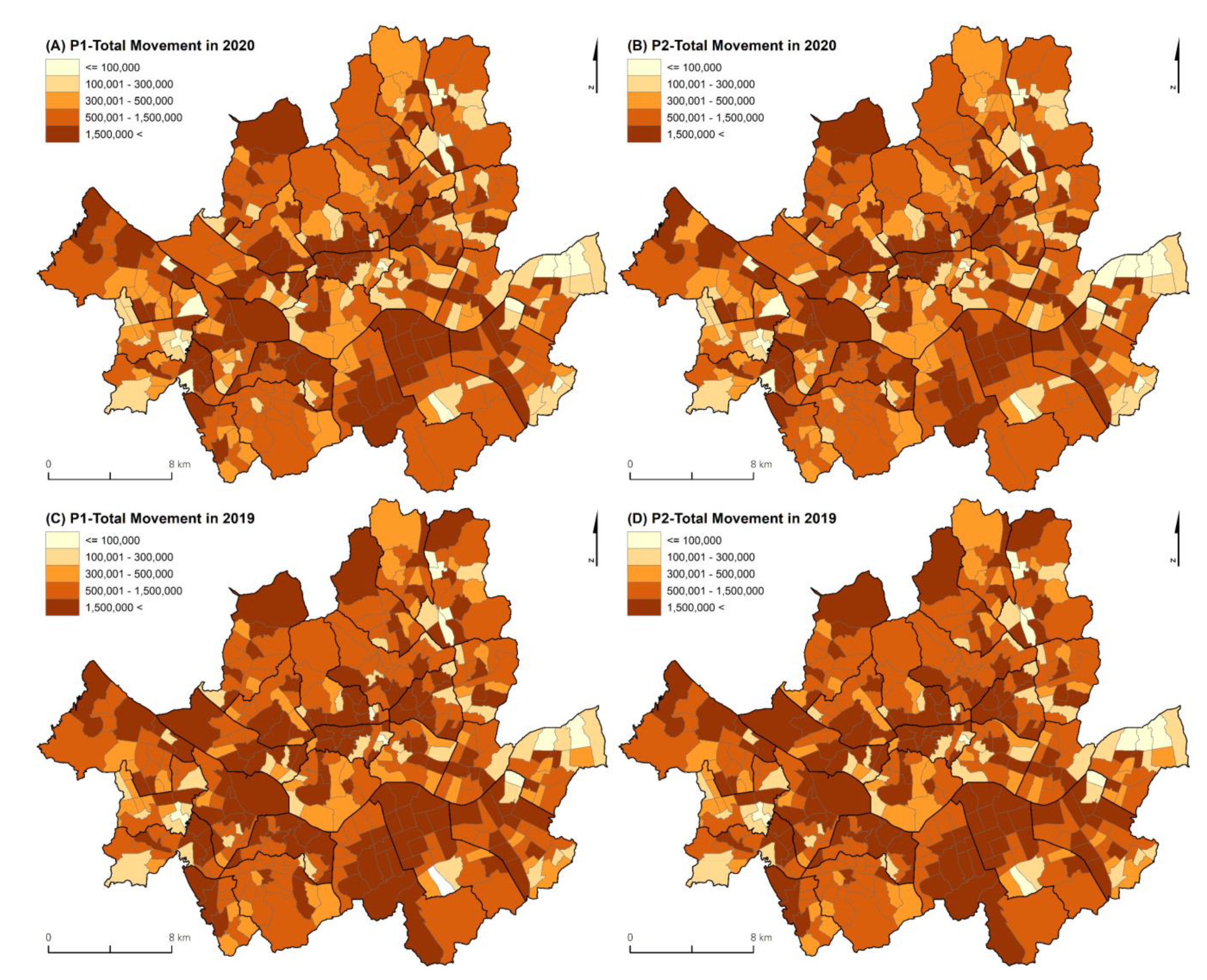
The monthly collected changes in restaurant sales (used for the dependent variables) showed significant differences between the two periods (Figure 2). The t-test between P1 and P2 verified the statistical significance of the difference in their means. Specifically, the changes in restaurant sales were generally below zero in P1 (Figure 3C), which means that the corresponding month in 2020 exhibited a decrease in restaurant sales compared with 2019. However, in P2, most regions showed changes of above zero percent (Figure 3D). That is, most regions showed an increase in restaurant sales during the COVID era. Only major commercial regions, e.g., Gangnam and Myeongdong, showed decreases in their sales during the whole period. This inconsistency in the relationship between population mobility and restaurant sales might indicate that a global regression model does not successfully explain the relationship during the whole period and study area. The spatial distributions of total population ridership are represented in Figure A1.
Table 2 presents the results of the global regression model between the changes in population mobility and restaurant sales. The regression model only explained a partial change variance of the proportion of sales in their corresponding mobility changes, with an adjusted R2 value of 0.294. This relatively low adjusted R2 value may denote that the relationship between the variables includes spatio-temporal heterogeneity. That is, because the global regression cannot capture the heterogeneity in the relationship between the variables, local regression models, e.g., MESF-based SVC models, were constructed for this analysis.
Although the explanatory power of this global regression model is low, statistically significant variables could reveal the general trends between population mobility and restaurant sales. The positively significant variables at the 0.1% confidence level were MD12 (0.0105), MD18 (0.0043), ME6 (0.0048), ME9 (0.0032), ME15 (0.0051), and ME21 (0.0068). Specifically, the decrease in the public transportation ridership during the 12–14 and 18–20 time periods on weekdays (i.e., MD12 and MD18, respectively) as well as the 6–8, 9–11, 15–17, and 21–23 time periods on weekends (i.e., ME6, ME9, ME15, and ME21, respectively) yielded a decrease in restaurant sales. Because MD12 and MD18 might reflect the population mobility for lunch and dinner, respectively, these positive relationships can be reasonably explained. In contrast to these variables, MD9 (−0.0073), MD21 (−0.0179), ME12 (−0.0073), and ME18 (−0.0057) had a significant negative relationship with the same confidence level. That is, the decrease in population mobility during 9–11 and 21–23 on weekdays as well as 12–14 and 18–20 on weekends instead produced an increase in sales. This means that the population mobility at these times might not be related to restaurant sales. For example, mobility during 9–11 and 21–23 on weekdays is caused by mobility for commutes to work.

4.2. Exploring Temporal Difference Using Statistical Interaction Terms

A statistical interaction term (i.e., dummy variable) was applied to the global regression model to capture the temporal variability in the relationships (Table 3). Here, this analysis applied zero for P1, i.e., from March to July, and applied one for P2, i.e., from August to December. The regression model with the interaction term showed a higher adjusted R2 value (0.678) than that of the global regression model without the interaction term (0.294). The partial F-test also reported a statistically significant difference between the two models. This result indicates that the variance in restaurant sales changes is better explained by the statistical interaction term; in other words, the statistical interaction term successfully explains the temporal heterogeneity in the relationships between the variables.
The estimated coefficients of the statistical interaction term marked with ‘INT’ (e.g., from MD6:INT to ME21:INT) represent the temporal difference in the relationships, which shows a remarkable difference in the relationship to the previous global regression model (Table 3). Based on the estimates of the interaction term with the two periods, the variables of MD12, MD18, MD21, ME12, ME15, and ME21 had noticeably different associations between the periods. The estimated regression coefficients without INT (e.g., from MD6 to ME21) report the relationship of restaurant sale changes to corresponding changes in population mobility for P1, and the sum of estimated coefficient with and without INT (e.g., the sum of MD6 and MD6:INT) represents the relationship for P2.
MD12 (i.e., mobility between 12–14 on weekdays) showed a negative relationship in P1 (i.e., −0.0009), but it had the opposite relationship in P2 (i.e., 0.0041). The differences were statistically significant at a 5% confidence level. That is, the changes in population mobility in P1 did not affect the changes in restaurant sales, but in P2, the mobility changes led to changes in their corresponding dependent variables. Because they have a positive relationship, the decrease in population mobility led to a decrease in restaurant sales. MD18 (i.e., mobility between 18–20 on weekdays) showed a similar interpretation to MD12. However, unlike MD12, MD18 showed a positive relationship in P1 (i.e., 0.0007), although it is not statistically significant. Nevertheless, similar to MD12, MD18 had a significantly different (i.e., stronger) relationship between P1 and P2 with a 1% confidence level. That is, in P1, a decrease in the mobility is related to a decrease in restaurant sales, and this relationship was intensified in P2. In whole periods, the decrease in local restaurant sales was globally more susceptible to mobility during dinner time than it was during lunch time.
The temporal changes of the relationship in MD21 (i.e., mobility between 21–23 on weekdays) are worth addressing despite the fact that the estimated coefficients for the related variables were not statistically significant. In the global regression model and model with the interaction terms in P1, MD21 had a negative relationship to restaurant sales, as the mobility in this time period is typically related to work commutes. However, in P2, MD21 showed a stronger negative relationship (i.e., −0.0049) to restaurant sales. This change might reflect the result of social distancing. Specifically, after August 16, as the level of social distancing increased to level 2, the social distancing policy allowed restaurants to provide delivery or takeout after 21:00. Thus, in P2, the mobility that was not related to restaurant sales tended to increase during 21–23 on weekdays.
The variables corresponding to mobility on weekends also had significantly different relationships with the changes in restaurant sales between P1 and P2. ME12 and ME15 (i.e., mobility between 12–14, and 15–17 on weekends, respectively) had opposite directions between P1 and P2. That is, in P1, ME12 had a positive relationship (0.0012) and ME15 had a negative relationship (−0.0028). Meanwhile ME12 in P2 showed a negative relationship (−0.0081), whereas ME15 had a positive relationship (0.0079). ME21 also exhibited significant changes in the estimated coefficients between P1 and P2 with a 10% confidence level. Specifically, ME21 (i.e., mobility between 21–23 on weekends) showed a significant positive relationship (0.0064) to restaurant sales in P1. The decrease in mobility during this time led to a decrease in restaurant sales until August. In P2, ME21 still showed a positive direction (0.0012), but there was a significant decrease in the estimated coefficient. This means that in the 21–23 time period on weekends, the mobility related to restaurant sales tended to decrease in P2 compared with P1, which might also have been caused by a change in the social distancing policy.

4.3. Exploring Spatio-Temporal Difference Using ESF-SVC with Statistical Interaction Terms

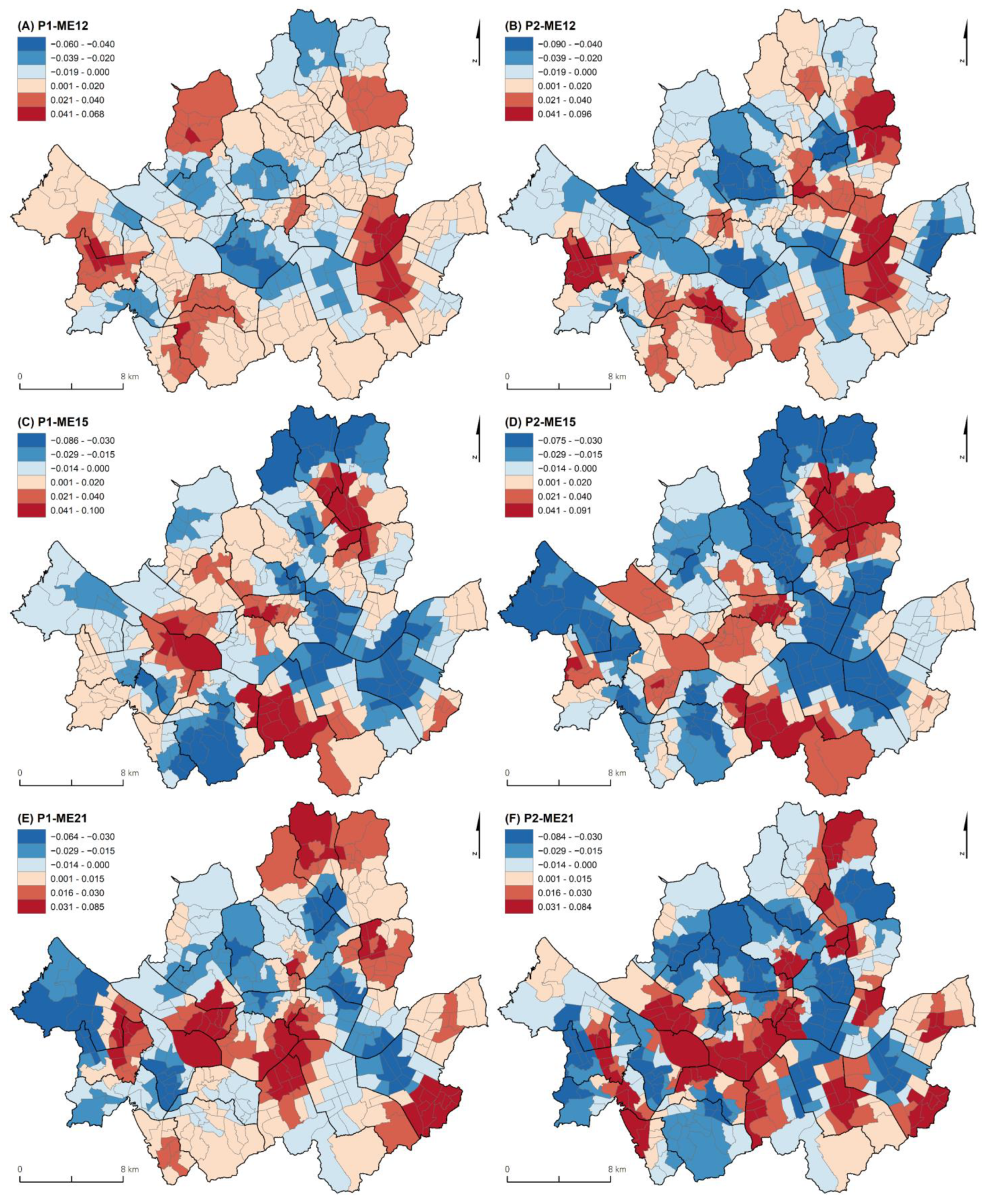
Temporal statistical interaction terms were applied to the local regression models, i.e., the MESF-SVC models, to explore the spatio-temporal variabilities in the relationship. Thus, the estimated coefficients varied by both location and period. The overall interpretation of coefficients is similar to their counterparts in the general regression coefficients. A positive relationship, i.e., an estimated coefficient that is larger than zero—denotes that a decrease in population mobility relates to a decrease in its corresponding local restaurant sales. By contrast, a negative relationship means that a decrease in population mobility tends to show an increase in its counterparts. Figure 4 and Figure 5 represent the spatially varying coefficients in P1 and P2 for weekdays (i.e., MD12, MD18, and MD21) and weekends (i.e., ME12, ME15, and ME21), respectively, which show noticeable relationships between the variables in the previous global regression model. In Figure 4 and Figure 5, the red and blue areas have positive and negative relationships, respectively.
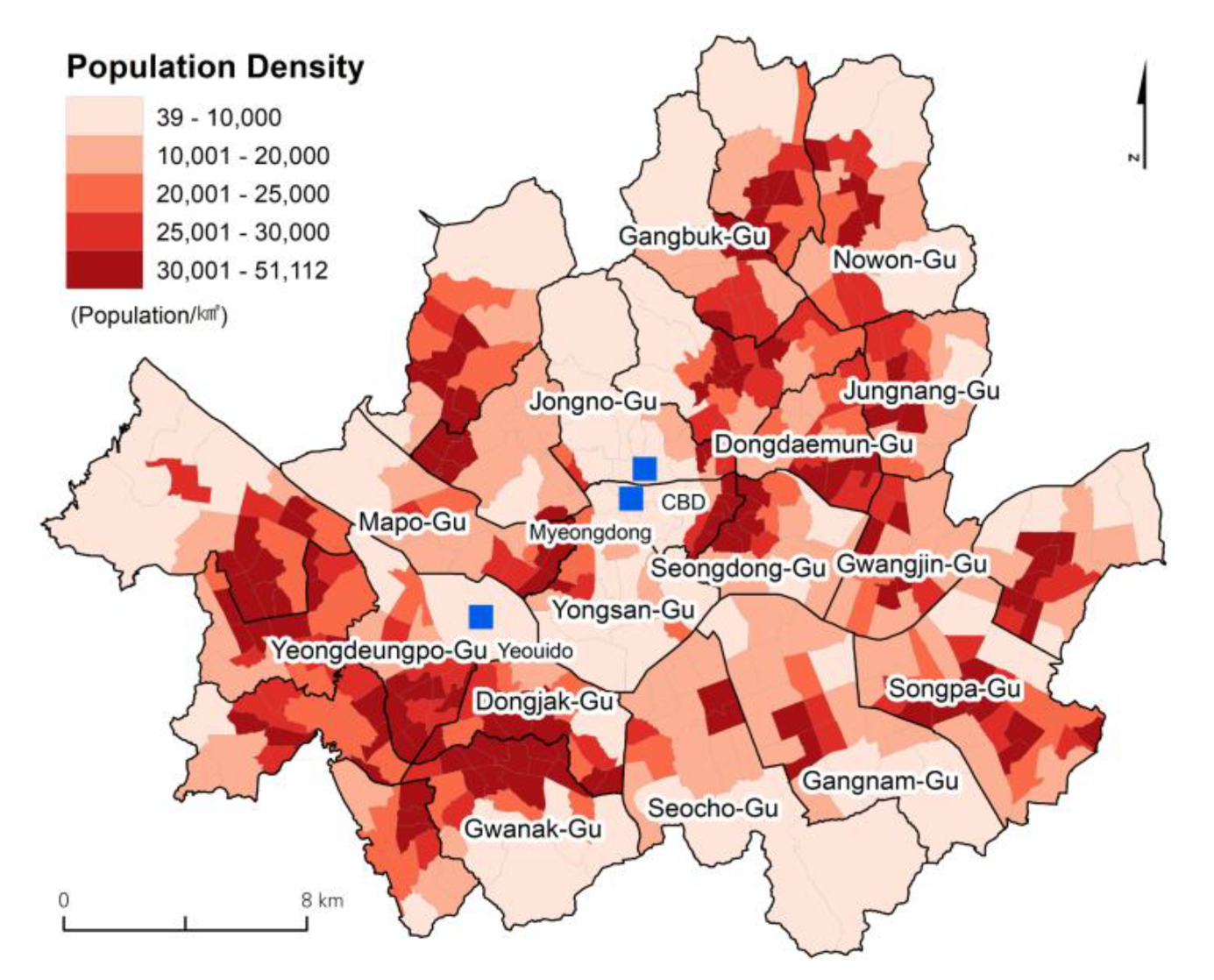
Although the coefficients of the global models for MD12 had negative and positive relationships in P1 and P2, respectively, where their MD12 SVC values showed various patterns according to the characteristics of their related regions (Figure 4A,B). The numbers of spatial units having a positive relationship in P1 and P2 were 199 and 259, respectively. For example, the central business area (CBD) in Seoul had negative coefficients during the whole period (See Figure 4A and Figure A2 for detailed regions). That is, the population mobility in this area decreased in 2020, but the decrease had no impact on local restaurant sales. Positive coefficients were mainly found in the neighboring areas of the CBD, where decreases in population mobility tended to cause a decrease in local restaurant sales. Regions having positive SVC values in P1 spread out in P2 (Figure 4B), which might lead to a positive relationship in the global model. Regions with positive SVC values were also observed in commercial areas such as Gangnam-Gu as well as residential areas such as Gangbuk-Gu and Jungnang-Gu. This analysis result shows that a decrease in population mobility during lunch time on weekdays had a larger negative impact on restaurant sales in commercial and residential areas than it does in the CBD, and regions with negative impacts expanded between the two periods.
The estimated coefficients of MD18 in the global regression model had positive relationships in both P1 and P2, but the SVC values of MD18 had spatio-temporally different patterns (Figure 4C,D). That is, 184 and 217 Dongs had positive relationships in P1 and P2, respectively. Generally, major commercial areas, e.g., Gangnam-Gu, Yongsan-Gu, and Yeouido, continuously represented positive SVC values, and the CBDs had negative SVC values. Thus, during dinner time, the decrease in mobility in these areas could decrease their local restaurant sales. Similar to the SVC values of MD12, the regions with positive SVC values were expanded in P2 compared with P1. In P2, most regions of Jongro-Gu, Gangbuk-Gu, and Seocho-Gu had positive SVC values (Figure 4D). This might mean that the negative impact of the mobility on restaurant sales was stronger in P2 than in P1, although the overall restaurant sales increased in P2.
The SVC values of MD21 included positive estimations (Figure 4E,F) for 199 and 259 Dongs for P1 and P2, respectively, although its global counterparts only had negative estimate coefficients (Table 3). The overall patterns of the MD21 SVC values were almost similar in both P1 and P2, but their intensities were generally larger in P2. That is, the absolute values of the MD21 SVC were larger in P2 compared with P1. In particular, regions with positive SVC values were observed in the CBD, where the negative SVC values were mostly found for MD12 and MD18. Because the mobility decrease in these time periods mainly reflected the changes in social distancing which only allowed restaurants to provide delivery or takeout in P2 [55], the regions with positive SVC values, e.g., Seongdong-Gu, Gwangjin-Gu, Dongdaemun-Gu, where commercial and residential areas are generally mixed, could be the major regions that suffered from the policy.
The SVC values of the variables related to the mobility on weekends, e.g., ME12, ME15, and ME21, showed different patterns to their corresponding mobility SVC on weekdays, e.g., MD12, MD15, and MD21 (Figure 5). The estimated coefficients of ME12 and ME15 in the global regression model exhibited opposite directions between P1 and P2, but the SVC patterns of ME12 and ME15 in both P1 and P2 were similar. Note that their absolute values were larger in P2 than in P1, which could lead to a significant difference in the estimated global regression coefficients between P1 and P2. Specifically, for ME12 (Figure 5A,B), the CBD and Yongsan-Gu mainly showed negative SVC, while the regions having positive SVC values were found in Gwangjin-Gu, Songpa-Gu, and Dongjak-Gu. For ME15 (Figure 5C,D), Gwanak-Gu, Gangnam-Gu, Songpa-Gu, and Seongdong-Gu represented negative SVC values, while Seocho-Gu and Nowon-Gu had positive SVC values. However, during the daytime on weekends, the positive SVC expanded from Myeongdong to the CBD in P2 compared with P1. This could indicate that the negative impact of decreasing population mobility on local restaurant sales spread out during P1.
The estimated coefficients of ME21 in the global regression model show positive relationships for both P1 and P2, but its SVC values include negative directions (Figure 5E,F). The regions having negative SVC values were expanded in P2—i.e., 195 and 223 Dongs for P1 and P2, respectively—and the absolute values of the SVC values were also larger in P2 compared with P1. The absolute values of the positive SVC values were also larger in P2, which includes Yongsan-Gu, Mapo-Gu, and Yeouido. As is the case for MD21, the decrease in population mobility in this time period, which was related to a decrease in local restaurant sales, was mainly caused as a result of the social distancing policy; because of this, the above-mentioned regions could also be considered to have suffered from the policy.

5. Conclusions

The social distancing policies implemented in response to COVID-19 could reduce population mobility, but could also lead to a change in local business sales in Seoul. This study explored the influences of the changes in population mobility on the changes in local restaurant sales, particularly from the perspectives of their spatio-temporal variabilities. First, a global regression model with a statistical interaction term was able to capture the temporal variability in the relationship between changes in population mobility and restaurant sales, which mainly occurred due to the changes in social distancing policies. In particular, the changes in population mobility at lunch and dinner times, i.e., between 12–14 and 18–20, had positive relationships on weekdays to their corresponding changes in restaurant sales from August to December (i.e., P1), which shows the negative impact of a decrease in population mobility on restaurant sales. In the same period, the changes in population mobility in the night time, i.e., between 21–23, showed negative relationships on both weekdays and weekends to the changes in restaurant sales. This could denote that mobility at this time was not related to restaurant sales and was caused by commuting to work, as the social distancing policy only allowed restaurants to provide delivery or take-out food and beverages.
Second, the MESF-based SVC models with statistical interaction terms were applied to explore the spatio-temporal variation in the impact of population mobility on local restaurant sales. Although the global regression model could only report a relationship between the related variables, the SVC models were able to represent various relationships related to the characteristics of the corresponding individual spatio-temporal units. For example, with the changes in population mobility at lunch time, i.e., between 12–14 on weekdays, the CBD and commercial areas, e.g., Gangnam-Gu, showed positive and negative coefficients in the whole period, respectively. Similar to this example, our analysis result showed that at this time, a decrease in population mobility had a larger impact on a decrease in restaurant sales in commercial areas than it did in the CBD. Because the decrease in population mobility at night, i.e., between 21–23, was mainly caused by the social distancing policy, the regions with positive SVC coefficients (which mean a decrease in population mobility) that tended to have a decrease in restaurant sales could be considered to be the major regions that suffered from the social distancing policies.
This article is expected to contribute to the literature on spatial analyses and policy supports in response to infectious disease, e.g., COVID-19. Methodologically, this study incorporated statistical interaction terms into MESF-based SVC models. In general, SVC models only explore spatially local regression coefficients, but our approach additionally verified the temporal variabilities of the spatial coefficients. This study also utilized spatial big data, such as the KCB and T-Money datasets, to examine the impact of population mobility changes on restaurant sales. The KCB and T-Money datasets were obtained from credit card transactions and transportation card histories, respectively. The analysis results confirmed the usability of spatial big data for the examination of socio-economic problems. Finally, this study estimates the changes in restaurant sales based on population mobility and discovered regions that suffered depending on the change in the social distancing policies. The results and our methodological approach could provide base research for policymakers by assisting in the prediction of the impact that social distancing policies have on local business sales in response to future infectious diseases.
This study could be extended in future research. First, this study only compared two periods, i.e., P1 from March to July and P2 from August to December. This is because the datasets used by this study show significantly different relationships between the related variables. Regression models could be incorporated with monthly statistical interaction terms to explore the detailed monthly variations of the relationships; however, it might yield difficulties with respect to interpreting the regression results. Moreover, linear mixed and panel models could be used as alternatives to examine the further relationships [46], although they might not be useful for this study due to the existence of significantly different relationships between the divisions. Second, multicollinearity exists between the independent variables, which could affect the significance tests of their estimated coefficients. An alternative representation of the time components, e.g., adjusting time periods, and subsequently extracting the principal components, may be helpful for future studies. Finally, the variants of the SARS-CoV-2 virus could yield different impacts on the changes in mobility and local restaurant sales, although this analysis only explored the impact observed in 2020. Exploring the changes in the impacts according to the emergence of the variants by comparing 2020 to 2022 would be helpful for understanding the overall responses of local business sales to the COVID-19 pandemic in Seoul, South Korea.

Supplementary Materials

The following are available online at https://www.mdpi.com/article/10.3390/ijgi11100532/s1.

Author Contributions

Conceptualization, Hyeongmo Koo, Jiyeong Lee and Daeheon Cho; formal analysis, Soyoung Lee; investigation, Soyoung Lee; supervision, Daeheon Cho; writing—original draft, Hyeongmo Koo and Soyoung Lee; writing—review and editing, Hyeongmo Koo, Jiyeong Lee and Daeheon Cho. All authors have read and agreed to the published version of the manuscript.

Funding

This work was supported by the 2021 Research Fund of the University of Seoul, Data Voucher Support program of the Korea Data Agency (2021-DV-I-P-00040), and National Research Foundation of Korea (NRF) grant funded by the Korea Government (MSIT) (2021R1C1C1007360).

Institutional Review Board Statement

Not applicable.

Informed Consent Statement

Not applicable.

Data Availability Statement

Restrictions apply to the availability of these data. Data was obtained from the Korea Credit Bureau (KCB).

Conflicts of Interest

The authors declare no conflict of interest.

Appendix A

Figure A1. Numbers of alighting population in 2019 for P1 (A) and P2 (B), and in 2020 for P1 (C) and P2 (D).
Ijgi 11 00532 g0a1
Figure A2. Study area and the highlighted regions.
Ijgi 11 00532 g0a2

References

  1. Drake, T.M.; Docherty, A.B.; Weiser, T.G.; Yule, S.; Sheikh, A.; Harrison, E.M. The Effects of Physical Distancing on Population Mobility during the COVID-19 Pandemic in the UK. Lancet Digit. Health 2020, 2, e385–e387. [Google Scholar] [CrossRef]
  2. Bonaccorsi, G.; Pierri, F.; Cinelli, M.; Flori, A.; Galeazzi, A.; Porcelli, F.; Schmidt, A.L.; Valensise, C.M.; Scala, A.; Quattrociocchi, W.; et al. Economic and Social Consequences of Human Mobility Restrictions under COVID-19. Proc. Natl. Acad. Sci. USA 2020, 117, 15530–15535. [Google Scholar] [CrossRef] [PubMed]
  3. Pepe, E.; Bajardi, P.; Gauvin, L.; Privitera, F.; Lake, B.; Cattuto, C.; Tizzoni, M. COVID-19 Outbreak Response, a Dataset to Assess Mobility Changes in Italy Following National Lockdown. Sci. Data 2020, 7, 3–9. [Google Scholar] [CrossRef]
  4. Nouvellet, P.; Bhatia, S.; Cori, A.; Ainslie, K.E.C.; Baguelin, M.; Bhatt, S.; Boonyasiri, A.; Brazeau, N.F.; Cattarino, L.; Cooper, L.V.; et al. Reduction in Mobility and COVID-19 Transmission. Nat. Commun. 2021, 12, 1–9. [Google Scholar] [CrossRef] [PubMed]
  5. Kraemer, M.U.G.; Yang, C.H.; Gutierrez, B.; Wu, C.H.; Klein, B.; Pigott, D.M.; du Plessis, L.; Faria, N.R.; Li, R.; Hanage, W.P.; et al. The Effect of Human Mobility and Control Measures on the COVID-19 Epidemic in China. Science 2020, 368, 493–497. [Google Scholar] [CrossRef]
  6. Badr, H.S.; Du, H.; Marshall, M.; Dong, E.; Squire, M.M.; Gardner, L.M. Association between Mobility Patterns and COVID-19 Transmission in the USA: A Mathematical Modelling Study. Lancet Infect. Dis. 2020, 20, 1247–1254. [Google Scholar] [CrossRef]
  7. Parino, F.; Zino, L.; Porfiri, M.; Rizzo, A. Modelling and Predicting the Effect of Social Distancing and Travel Restrictions on COVID-19 Spreading. J. R. Soc. Interface 2021, 18, 20200875. [Google Scholar] [CrossRef]
  8. Lewnard, J.A.; Lo, N.C. Scientific and Ethical Basis for Social-Distancing Interventions against COVID-19. Lancet Infect. Dis. 2020, 3099, 631–633. [Google Scholar] [CrossRef]
  9. Wellenius, G.A.; Vispute, S.; Espinosa, V.; Fabrikant, A.; Tsai, T.C.; Hennessy, J.; Dai, A.; Williams, B.; Gadepalli, K.; Boulanger, A.; et al. Impacts of Social Distancing Policies on Mobility and COVID-19 Case Growth in the U.S. Nat. Commun. 2021, 12, 6–12. [Google Scholar] [CrossRef]
  10. De Vos, J. The Effect of COVID-19 and Subsequent Social Distancing on Travel Behavior. Transp. Res. Interdiscip. Perspect. 2020, 5, 100121. [Google Scholar] [CrossRef] [PubMed]
  11. Jenelius, E.; Cebecauer, M. Impacts of COVID-19 on Public Transport Ridership in Sweden: Analysis of Ticket Validations, Sales and Passenger Counts. Transp. Res. Interdiscip. Perspect. 2020, 8, 100242. [Google Scholar] [CrossRef] [PubMed]
  12. Kim, J.; Kwan, M.P. The Impact of the COVID-19 Pandemic on People’s Mobility: A Longitudinal Study of the U.S. from March to September of 2020. J. Transp. Geogr. 2021, 93, 103039. [Google Scholar] [CrossRef]
  13. Park, J. Changes in Subway Ridership in Response to COVID-19 in Seoul, South Korea: Implications for Social Distancing. Cureus 2020, 14, e7668. [Google Scholar] [CrossRef] [PubMed]
  14. Lee, K.; Park, S.; Ham, Y. Changes in Subway Traffic in Seoul during Social Distancing Due to the Spread of COVID-19 and Geographic Characteristics of the Area behind the Station. J. Econ. Geogr. Soc. Korea 2021, 24, 127–142. [Google Scholar]
  15. Lee, H.; Park, S.J.; Lee, G.R.; Kim, J.E.; Lee, J.H.; Jung, Y.; Nam, E.W. The Relationship between Trends in COVID-19 Prevalence and Traffic Levels in South Korea. Int. J. Infect. Dis. 2020, 96, 399–407. [Google Scholar] [CrossRef]
  16. Zhu, R.; Anselin, L.; Batty, M.; Kwan, M.P.; Chen, M.; Luo, W.; Cheng, T.; Lim, C.K.; Santi, P.; Cheng, C.; et al. The Effects of Different Travel Modes and Travel Destinations on COVID-19 Transmission in Global Cities. Sci. Bull. 2022, 67, 588–592. [Google Scholar] [CrossRef]
  17. Carracedo, P.; Puertas, R.; Marti, L. Research Lines on the Impact of the COVID-19 Pandemic on Business. A Text Mining Analysis. J. Bus. Res. 2021, 132, 586–593. [Google Scholar] [CrossRef]
  18. Pantano, E.; Pizzi, G.; Scarpi, D.; Dennis, C. Competing during a Pandemic? Retailers’ Ups and Downs during the COVID-19 Outbreak. J. Bus. Res. 2020, 116, 209–213. [Google Scholar] [CrossRef]
  19. Panzone, L.A.; Larcom, S.; She, P.W. Estimating the Impact of the First COVID-19 Lockdown on UK Food Retailers and the Restaurant Sector. Glob. Food Sec. 2021, 28, 100495. [Google Scholar] [CrossRef]
  20. Fairlie, R. The Impact of COVID-19 on Small Business Owners: Evidence from the First Three Months after Widespread Social-Distancing Restrictions. J. Econ. Manag. Strateg. 2020, 29, 727–740. [Google Scholar] [CrossRef]
  21. Na, H.; Kim, J.; Ahn, J.; Na, H.; Kim, J.; Ahn, J.; Jun, D.; Im, D. Analyzing Relationships between Floating Population and Card Consuming Data in Seoul before and after COVID-19. Proc. Korea Inf. Process. Soc. Conf. 2021, 28, 301–304. [Google Scholar]
  22. Lim, S.; Lim, H.; Després, J.P. Collateral Damage of the COVID-19 Pandemic on Nutritional Quality and Physical Activity: Perspective from South Korea. Obesity 2020, 28, 1788–1790. [Google Scholar] [CrossRef] [PubMed]
  23. Chang, S.-J.; Park, J.-M.; Kang, J.-Y. A Study on the Effect the Infected Number of COVID-19 on the Number of Food Deliveries: Focusing on the Mediating Effect of the National Disaster Fund and Social Distancing. Korea Int. Trade Res. Inst. 2022, 18, 131–147. [Google Scholar] [CrossRef]
  24. Jin, J.; Seong, B. Analysis of the Differences in Living Population Changes and Regional Responses by COVID-19 Outbreak in Seoul. Korean J. Appl. Stat. 2020, 33, 697–712. [Google Scholar]
  25. Ryu, E.H.; Kim, E.J. Analysis of the Changes in de Facto Population Pattern and Effects of Local Environment on Changes in the de Facto Population in Seoul after the COVID-19. J. Korean Urban Geogr. Soc. 2021, 24, 19–35. [Google Scholar] [CrossRef]
  26. Yellow Horse, A.J.; Yang, T.C.; Huyser, K.R. Structural Inequalities Established the Architecture for COVID-19 Pandemic among Native Americans in Arizona: A Geographically Weighted Regression Perspective. J. Racial Ethn. Health Disparities 2022, 9, 165–175. [Google Scholar] [CrossRef]
  27. Wu, X.; Zhang, J. Exploration of Spatial-Temporal Varying Impacts on COVID-19 Cumulative Case in Texas Using Geographically Weighted Regression (GWR). Environ. Sci. Pollut. Res. 2021, 28, 43732–43746. [Google Scholar] [CrossRef]
  28. Jiao, J.; Chen, Y.; Azimian, A. Exploring Temporal Varying Demographic and Economic Disparities in COVID-19 Infections in Four U.S. Areas: Based on OLS, GWR, and Random Forest Models. Comput. Urban Sci. 2021, 1, 27. [Google Scholar] [CrossRef]
  29. Chen, M.; Chen, Y.; Wilson, J.P.; Tan, H.; Chu, T. Using an Eigenvector Spatial Filtering-Based Satially Varying Coefficient Model to Analyze the Spatial Heterogeneity of COVID-19 and Its Influencing Factors in Mainland China. ISPRS Int. J. Geo-Inf. 2022, 11, 67. [Google Scholar] [CrossRef]
  30. Koo, H. Exploring Spatial Heterogeneity in Factors for Apartment Prices in Seoul Using Moran Eigenvector Spatial Filtering Based on Spatially Varying Coefficients. J. Assoc. Korean Geogr. 2019, 8, 321–335. [Google Scholar] [CrossRef]
  31. Lee, J.; Kim, G.C. The Smart Transportation Card (T-Money): Integrating Public Transit Systems to Improve Citizen Mobility in Seoul, 1996–2004. Glob. Deliv. Initiat. 2021, 1, 1–12. [Google Scholar]
  32. Ha, E.; Lee, C.; Koh, M.; Kim, K. The Differential Effect of COVID-19 on Mobility. J. Korean Cartogr. Assoc. 2021, 21, 59–76. [Google Scholar] [CrossRef]
  33. Yang, S.; Jang, J.; Park, S.Y.; Ahn, S.H.; Kim, S.; Park, S.B.; Ryu, B.; Lee, S.; Shin, E.; Kim, N.-Y.; et al. COVID-19 Outbreak Report from January 20, 2020 to January 19, 2022 in the Republic of Korea. Public Health Wkly. Rep. 2022, 15, 796–805. [Google Scholar]
  34. Task Force for Tackling COVID-19. All about Korea’s Response to COVID-19; Ministry of Foreign Affairs: Seoul, Korea, 2020. [Google Scholar]
  35. Madeira, A.; Palrão, T.; Mendes, A.S. The Impact of Pandemic Crisis on the Restaurant Business. Sustainability 2021, 13, 40. [Google Scholar] [CrossRef]
  36. Lee, J.H.; Park, M.S.; Lee, S. The Transmission Dynamics of SARS-CoV-2 by Setting in Three Waves in the Seoul Metropolitan Area in South Korea. Health Soc. Welf. Rev. 2021, 41, 7–26. [Google Scholar]
  37. Kim, J.; Ki, D.; Lee, S. Analysis of Travel Mode Choice Change by the Spread of COVID-19: The Case of Seoul, Korea. J. Korea Plan. Assoc. 2021, 56, 113–129. [Google Scholar] [CrossRef]
  38. James, G.; Witten, D.; Hastie, T.; Tibshirani, R. An Introduction to Statistical Learning with Applications in R; Springer: New York, NY, USA, 2017. [Google Scholar]
  39. Chun, Y.; Griffith, D.A. Spatial Statistics and Geostatistics: Theory and Applications for Geographic Information Science and Technology; Sage Publications Inc.: London, UK, 2013; ISBN 1446201732. [Google Scholar]
  40. Koo, H.; Chun, Y.; Griffith, D.A. Modeling Positional Uncertainty Acquired through Street Geocoding. Int. J. Appl. Geospatial Res. 2018, 9, 1–22. [Google Scholar] [CrossRef]
  41. Franch-Pardo, I.; Napoletano, B.M.; Rosete-Verges, F.; Billa, L. Spatial Analysis and GIS in the Study of COVID-19. A Review. Sci. Total Environ. 2020, 739, 140033. [Google Scholar] [CrossRef]
  42. Franch-Pardo, I.; Desjardins, M.R.; Barea-Navarro, I.; Cerdà, A. A Review of GIS Methodologies to Analyze the Dynamics of COVID-19 in the Second Half of 2020. Trans. GIS 2021, 25, 2191–2239. [Google Scholar] [CrossRef]
  43. Helbich, M.; Griffith, D.A. Spatially Varying Coefficient Models in Real Estate: Eigenvector Spatial Filtering and Alternative Approaches. Comput. Environ. Urban Syst. 2016, 57, 1–11. [Google Scholar] [CrossRef]
  44. Griffith, D.A. Spatial Autocorrelation and Spatial Filtering: Gaining Understanding through Theory and Scientific Visualization; Springer: Berlin/Heidelberg, Germany, 2003; ISBN 3540248064. [Google Scholar]
  45. Chun, Y.; Griffith, D.A. Modeling Network Autocorrelation in Space-Time Migration Flow Data: An Eigenvector Spatial Filtering Approach. Ann. Assoc. Am. Geogr. 2011, 101, 523–536. [Google Scholar] [CrossRef]
  46. Chun, Y. Analyzing Space-Time Crime Incidents Using Eigenvector Spatial Filtering: An Application to Vehicle Burglary. Geogr. Anal. 2014, 46, 165–184. [Google Scholar] [CrossRef]
  47. Tiefelsdorf, M.; Boots, B. The Exact Distribution of Moran’s I. Environ. Plan. A 1995, 27, 985–999. [Google Scholar] [CrossRef]
  48. Griffith, D.A. Eigenfunction Properties and Approximations of Selected Incidence Matrices Employed in Spatial Analyses. Linear Algebra Appl. 2000, 321, 95–112. [Google Scholar] [CrossRef]
  49. Wheeler, D.; Tiefelsdorf, M. Multicollinearity and Correlation among Local Regression Coefficients in Geographically Weighted Regression. J. Geogr. Syst. 2005, 7, 161–187. [Google Scholar] [CrossRef]
  50. Murakami, D.; Lu, B.; Harris, P.; Brunsdon, C.; Charlton, M.; Nakaya, T.; Griffith, D.A. The Importance of Scale in Spatially Varying Coefficient Modeling. Ann. Am. Assoc. Geogr. 2019, 109, 50–70. [Google Scholar] [CrossRef]
  51. Murakami, D.; Yoshida, T.; Seya, H.; Griffith, D.A.; Yamagata, Y. A Moran Coefficient-Based Mixed Effects Approach to Investigate Spatially Varying Relationships. Spat. Stat. 2017, 19, 68–89. [Google Scholar] [CrossRef]
  52. Griffith, D.A. Spatial-Filtering-Based Contributions to a Critique of Geographically Weighted Regression (GWR). Environ. Plan. A 2008, 40, 2751–2769. [Google Scholar] [CrossRef]
  53. Chun, Y.; Griffith, D.A.; Lee, M.; Sinha, P. Eigenvector Selection with Stepwise Regression Techniques to Construct Eigenvector Spatial Filters. J. Geogr. Syst. 2016, 18, 67–85. [Google Scholar] [CrossRef]
  54. Tiefelsdorf, M.; Griffith, D.A. Semiparametric Filtering of Spatial Autocorrelation: The Eigenvector Approach. Environ. Plan. A 2007, 39, 1193–1221. [Google Scholar] [CrossRef]
  55. Kim, S.; Kim, Y.J.; Peck, K.R.; Ko, Y.; Lee, J.; Jung, E. Keeping Low Reproductive Number despite the Rebound Population Mobility in Korea, a Country Never under Lockdown during the Covid-19 Pandemic. Int. J. Environ. Res. Public Health 2020, 17, 9551. [Google Scholar] [CrossRef] [PubMed]
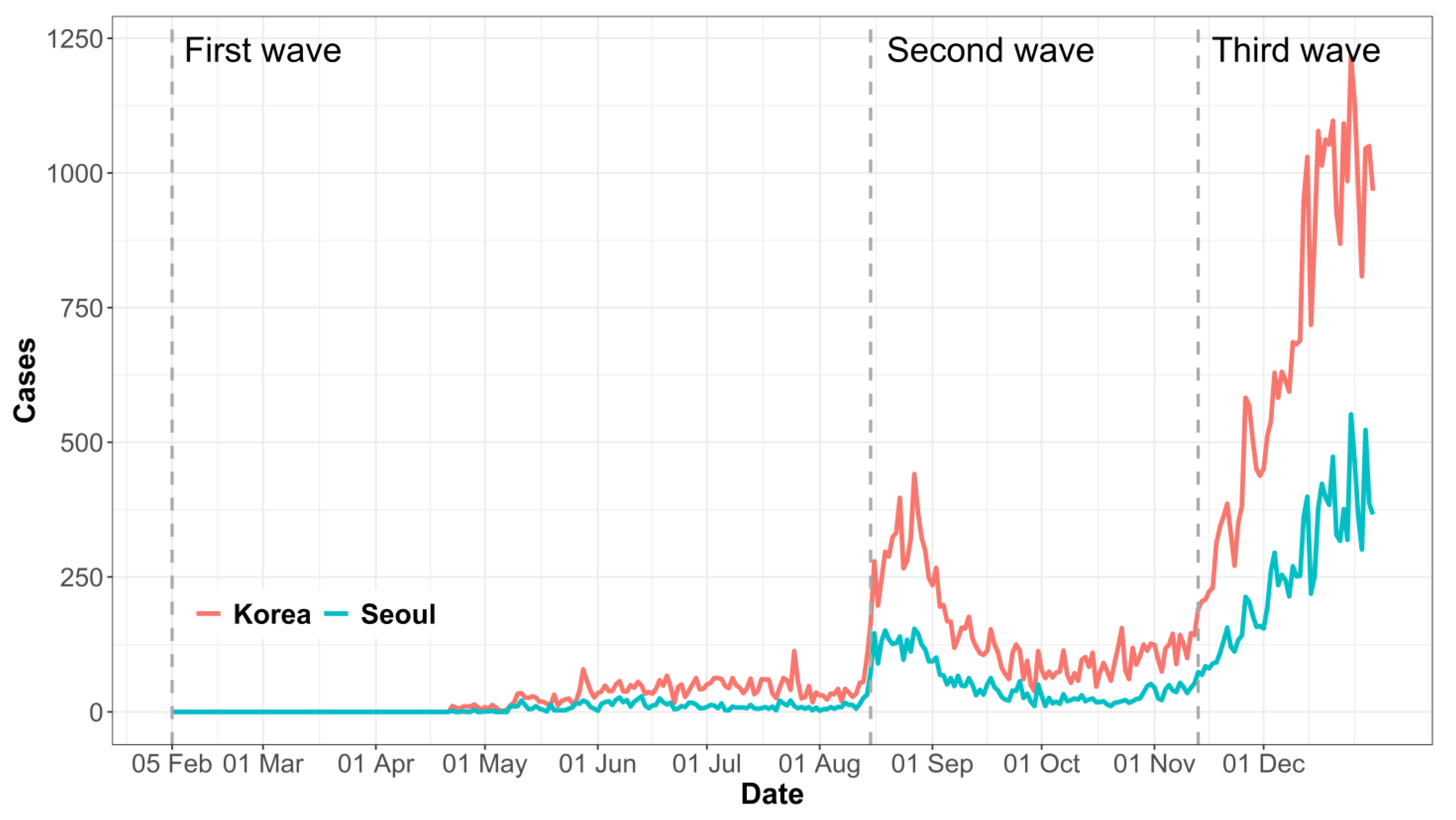
Figure 1. Numbers of newly confirmed COVID-19 cases in 2020.
Ijgi 11 00532 g001
Figure 2. Monthly changes in the population mobility and restaurant sales.
Ijgi 11 00532 g002
Figure 3. Spatial distributions of the changes in population mobility and restaurant sales; the change in population mobility for P1 (A) and for P2 (B), and the change in restaurant sales for P1 (C) and for P2 (D).
Ijgi 11 00532 g003
Figure 4. Spatio-temporally varying coefficients of location mobility on weekdays; (A) MD12 in P1, (B) MD12 in P2, (C) MD18 in P1, (D) MD18 in P2, (E) MD21 in P1, and (F) MD21 in P2.
Ijgi 11 00532 g004
Figure 5. Spatio-temporally varying coefficients of population mobility on weekends; (A) ME12 in P1, (B) ME12 in P2, (C) ME15 in P1, (D) ME15 in P2, (E) MD21 in P1, and (F) MD21 in P2.
Ijgi 11 00532 g005
Table 1. Implementation of social distancing policies in Seoul, 2020.
PeriodsChanges in Social Distancing Policies
DatesImplemented Policies
First wave22 MarchStronger social distancing: postponing or canceling nonessential gatherings, dining out, and travel; in the case of an employer, using flexible work schedules, or adjusting start/end times of work and lunch hours
6 MayDistancing in daily life: harmonizing daily life and infection prevention against the possibility of the long-term prevalence of COVID-19, providing personal guidance suggestions, e.g., staying at home for 3–4 days if unwell and maintaining a distance from others.
28 JuneImplementation of the three-level social distancing policy
Second wave16 AugustLevel 2 of social distancing: avoiding unnecessary outings, meetings, and multi-use facilities; assemblies of no more than 50 people indoors and 100 people outdoors; recommendation of flexible work arrangements (taking lunch breaks in turn) or telecommuting to minimize place density
30 AugustEnhanced level 2 social distancing: only allowing restaurants and cafes to provide delivery or takeout after 21:00 (franchise cafes only permitted to offer takeout and delivery at all times)
14 SeptemberLevel 2 of social distancing: rather than restricting cafes and restaurants to take-out and delivery services, spacing is maintained between tables and seats to limit the number of people in a store (recording the lists of visitors for facilities, wearing of masks)
12 OctoberLevel 1 of social distancing: complying with quarantine guidelines and permitting daily economic activities; allowing assemblies, gatherings, and events, but recommending compliance with quarantine rules and imposing restrictions on the use of high-risk facilities
7 NovemberImplementation of the five-level social distancing policy
Third wave19 NovemberLevel 1.5 of social distancing: as social distancing was enhanced to level 1.5, the scope of restaurants and cafes was expanded (150 m2 → 50 m2 + facilities)
24 NovemberLevel 2 of social distancing: only take-out and delivery permitted after 21:00 (restaurant, all beverage-selling cafes, including franchises); one meter distance between tables, one seat/table space apart or partitions between tables (50 m2 + facilities)
8 DecemberLevel 2.5 of social distancing
(23 December: Private gatherings of more than five people were prohibited)
Table 2. Summary of the global linear regression result.
VariablesEstimateStandard Errort-Valuep-Value
(Intercept)−0.14620.0297−4.923<0.001 ***
MD60.00020.00090.1810.856
MD9−0.00730.0009−7.834<0.001 ***
MD120.01050.00166.551<0.001 ***
MD150.00290.00191.5180.13
MD180.00430.00113.811<0.001 ***
MD21−0.01790.0019−9.255<0.001 ***
ME60.00480.00085.801<0.001 ***
ME90.00320.00103.0670.002 **
ME12−0.00730.0016−4.611<0.001 ***
ME150.00510.00182.7860.005 **
ME18−0.00570.0019−3.0160.003 **
ME210.00680.00213.210.001 **
Adjusted R20.2941
F-test30.27 on 12 and 831 degrees of freedom, p-value: <0.001
Note: Significance codes: *** 0.001, ** 0.01, * 0.05.
Table 3. Summary of the linear regression result with the statistical interaction terms.
VariablesEstimateStandard Errort-Valuep-Value
(Intercept)0.02940.02301.27500.203
MD6−0.00090.0008−1.03400.302
MD9−0.00110.0009−1.22900.22
MD12−0.00090.0016−0.57600.565
MD150.00180.00180.98400.325
MD180.00070.00110.65800.511
MD21−0.00120.0019−0.62300.534
ME60.00160.00081.89700.058.
ME90.00140.00101.46100.144
ME120.00120.00170.71900.473
ME15−0.00280.0019−1.52000.129
ME18−0.00160.0019−0.82700.409
ME210.00640.00193.3030<0.001 ***
MD6:INT0.00010.00130.04700.962
MD9:INT−0.00080.0014−0.60300.546
MD12:INT0.00500.00232.17900.03 *
MD15:INT−0.00380.0027−1.38600.166
MD18:INT0.00410.00152.71300.007 **
MD21:INT−0.00370.0031−1.19100.234
ME6:INT−0.00010.0012−0.09500.924
ME9:INT0.00240.00151.60800.108
ME12:INT−0.00930.0023−4.1110<0.001 ***
ME15:INT0.01070.00264.1000<0.001 ***
ME18:INT−0.00410.0025−1.62300.105
ME21:INT−0.00520.0031−1.68900.092
Adjusted R20.6783
F-test65.75 on 24 and 819 degree of freedom, p-value: <0.001
Note: Significance codes: *** 0.001, ** 0.01, * 0.05.
Publisher’s Note: MDPI stays neutral with regard to jurisdictional claims in published maps and institutional affiliations.