Influence of Varied Ambient Population Distribution on Spatial Pattern of Theft from the Person: The Perspective from Activity Space

Abstract

The ambient population has been regarded as an important indicator for analyzing or predicting thefts. However, the literature has taken it as a homogenous group and seldom explored the varied impacts of different kinds of ambient populations on thefts. To fill this gap, supported by mobile phone trajectory data, this research investigated the relationship between ambient populations of different social groups and theft in a major city in China. With the control variables of motivated offenders and guardianship, spatial-lag negative binominal models were built to explore the effects of the ambient populations of different social groups on the distribution of theft. The results found that the influences of ambient populations of different social groups on the spatial distribution of theft are different. Accounting for the difference in the “risk–benefit” characteristics among different activity groups to the offenders, individuals from the migrant population are the most likely to be potential victims, followed by suburban and middle-income groups, while college, affluent, and affordable housing populations are the least likely. The local elderly population had no significant impact. This research has further enriched the studies of time geography and deepened routine activity theory. It suggests that the focus of crime prevention and control strategies developed by police departments should shift from the residential space to the activity space.

1. Introduction

Theft from the person (hereinafter referred to as “theft”) is closely related to human activity because it concerns individual belongings. According to the routine activity theory, theft is often the consequence of the convergence of motivated offenders, potential victims, and the absence of guardianship under specific circumstances [1,2]. How to measure these three factors, as well as the environment, in order to explain the spatial pattern and mechanism of theft, has become a topic of interest in the literature. In the geography of crime, one of the hot topics is how to measure the victim. Many previous studies measured victims through census data [3,4]. However, as people moved around the space, the static data could not explicitly measure the real population distribution. The ambient population, which refers to the demographics and volumes of people in a particular location throughout the day dynamically, has been regarded as an important indicator for analyzing or predicting thefts [5]. However, the literature has taken it as a homogenous group and seldom explored the varied impacts of different kinds of ambient populations on theft. By using mobile phone big data, this study aimed to investigate the effects of different ambient populations on the spatial distribution of theft.

At present, many studies use the residential population from the census, POI (point of interest), and land-use types to measure human activity and, therefore, indirectly measure potential victims [6,7,8,9]. However, these static data cannot reflect the dynamic population in a region. For example, Boggs et al. found that potential victims could not be effectively measured if residents left their homes for work and leisure activities because the number of residents was not equal to the ambient population in the region, due to the influence of the daily mobility of residents [10]. Although the number of residents in the commercial community is small, there are a large number of ambient populations in the community. As a result, theft occurs very frequently here [11,12]. It can be seen that the actual ambient population in a region has a larger influence on theft than the nominal residents in the region.

The widespread use of big data has provided a new way to study the ambient population in a region more accurately. In recent years, many scholars have used the big data produced by the instance of social media and mobile phones to recognize ambient populations and further measure potential victims. Although all populations could be both potential victims and potential offenders, studies often regard the ambient population as potential victims because most of the population has the risk of being stolen from, while only a few people have the tendency to steal things from others [4]. For example, Lan et al. found that Twitter data could be used to measure potential victims of theft well [12]; Malleson et al. compared the violent crime rate that was calculated based on Twitter user data and the resident population and found a large difference in the spatial pattern of crime hotspots among different calculation methods [13], and used the correlation coefficient in the subsequent study to compare the validity of mobile user density and other ambient population indexes (including the resident population in the demographic census and Twitter data) in analyzing the spatial pattern of violent crime. The same should hold for theft. In a study based in London, it was found that Twitter data could be used to measure potential victims more accurately [14]. Song et al. selected ZG City in China as the study area by comparing the mobile phone data, resident population data from the census, subway population, and GPS data from taxis, and found that the GPS data from taxis and mobile phone data could be used to measure potential victims in the afternoon and at night more accurately [3].

According to the above studies, it is better to represent potential victims by measuring the ambient population rather than the resident population or POI data, because the former can explain the spatial distribution of crime well. Existing studies cannot distinguish the properties of the population but consider them as homogenous potential victims. According to rational choice theory, offenders often make decisions with consideration of their benefit, risk, and cost [15]. For example, Xiao et al. found that residential burglars abided by the rule of “Safety First, benefit Second” [16]. This should also be applied to theft from the person. Ambient populations with different social attributes may lead to different benefits, risks, and costs to offenders. As a result, they have different influences on theft. For example, Song et al. used the principal component analysis method to extract social principal factors from the census and discussed the influence of different social factors on theft [7]. It was found that different social populations had different wealth attractions for offenders, and their social control effects are dissimilar, leading to different influences on theft. However, the research cannot reflect spatial activity variation in different populations due to the static demographic census data and cannot further study the influence of different populations on theft from the view of activity space.

Compared to the traditional census or survey data, although big data feature wide population coverage, high spatial resolution, and low acquisition cost [17], big data cannot measure and classify the detailed attributes of populations due to the lack of attribute information of individuals. In a study based in Barcelona, Spain, the authors divided ambient populations into tourists and residential populations [18]; in a study based in Beijing, China, residents, visitors, and employees were classified based on the ambient population [19], but the social attributes for the ambient population were still missing.

In contrast, traditional data can be used to classify different populations as their registered residence, age, income, and occupation. How to combine the advantages of big data and traditional data to study the influence of activity space distribution of different populations on the spatial pattern of crime will be a hot topic in the study of measuring victims.

Moreover, individuals with similar social and economic attributes may inhabit the same community. That is, individual attributes have a strong correlation with his/her place of residence [20,21]. Therefore, it is possible to classify the population as per their places of residence. For example, Zhou et al. classified Guangzhou into several groups based on the census, including middle-income community, low-income community, urban population community, intellectual community, etc. [22]. Hirschfield et al. used different types of neighborhoods identified by the census to investigate their impact on crime [20]. The mobility or the actual presence of the residents from different social areas can have diverse impacts on theft. In other words, the relationship between ambient populations of different social groups and theft is still unknown.

Therefore, to fill this gap, this research first classified different communities based on the census, recognized the residences of mobile users, and provided related attributes to them based on the traits of their place of residence. Then, the populations in different communities were calculated based on the activity trajectory (node) of mobile users. On this basis, this research explored the influence of ambient populations with different features on the spatial pattern of theft.

2. Data and Method

ZG City, located in southern China, has a population of more than 10 million, according to the 2010 census. Due to a confidential agreement, we used “ZG City” instead of its real name here. As one of the megacities in China, ZG City has complete infrastructure, a high distribution density of mobile base stations, and a good police–geographic information system (PGIS) and data foundation. According to the 2010 census, there are a total of 2643 communities among 12 districts in ZG City. Since three districts are located in the outer suburbs and the urban appearance is different from the other nine districts, they were removed from the analysis. Thus, only nine districts with 1530 communities with an average area of 1.558 km² were included in the analysis. We used the community as the unit of analysis because the socioeconomic attributes and geographical environment of the people within the community were relatively consistent.

Compared to the geography of crime analysis in other cities, for example, in the Hague, the Netherlands, the spatial analysis unit is 142 four-digit postal code areas, with an average population of 7000 and 2.96 km² for each area [23]. While in Brisbane, Australia, the mean statistical study area is 8.48 km², with an average of 299 households per km² [24,25]. In the West Midlands in the UK, the census lower-level super output area (LSOA) is the basic spatial unit, with approximately 1500 residents and 0.51 km² for each LSOA [26]. Additionally, in Chicago, USA, the mean area for the census tracts is approximately 140 m × 140 m, with an average population of 118 residents [27]. Undoubtedly, the population density is much higher in ZG City compared to the above-mentioned western cities. However, the spatial unit for crime analysis in ZG City is similar to the others.

2.1. Data Source

In this research, the dependent variable was the number of thefts in each community, which was taken from workday data of theft from the public security bureau in ZG City in 2016. Although there were several analyses using the crime rate as the dependent variable, there was no consensus on the denominator. While the numerator was the number of theft, the denominators could be area, residential population or ambient population [28,29]. However, following most of the crime geography studies, the number of thefts was used as the dependent variable in this study. Other variables were obtained from the 6th census from the statistics bureau, points of interest from a navigation company, and mobile phone data from a mobile company, Unicom.

The mobile phone data only included one day on 28 December 2016 (Wednesday, workday) after desensitization processing by China Unicom in ZG City, and did not include the social economic attributes of the individual. As we only had one day’s data, to keep time consistency, we also chose the theft data from a workday in 2016. 28 December 2016 was a usual workday in China as there was no Christmas holiday on this day.

The mobile phone data included the position of the base station for each user at different moments. At most, one base station point was retained for each user in each hour, and the geographic location of the user at the time was the community, where the base station point with the maximum stay duration for the user could be found. For example, from 9:00 a.m. to 10:00 a.m., if a user I stays for 20 min in the service area of base station A, stays for 10 min in the service area of base station B, and stays for 30 min in the service area of base station C, it was considered that the location of the user I in the period was the community of base station C. The calculation method is shown in the following section.

2.2. Method of Population Type Division

Indeed, every person has their own attributes. In this study, we assigned the attributes of each community to the residents who were living in the community. However, residents move around, not only in their residential community, but also in other communities. Thus, we calculated how the residents moved around the communities throughout the whole day (24 h). Then, as each person had their own attribute based on where they lived (a total of seven attributes based on the following clustering method), we calculated, for each community, how many persons with different kinds of attributes had ever stayed there.

The method of population type division included two parts: (1) division of social area for each community; and (2) division of ambient population type.

(1)

Division of social area for each community

Referring to the classification method used by Zhou et al. [22], the research first implemented principal component analysis (PCA) for the 6th census, then extracted and used the principal factors for clustering analysis to classify the communities. The research selected 35 indexes from the 6th census for PCA. The 35 indexes from the census were attributes containing population characteristics as well as housing characteristics. With regard to population characteristics, variables such as hukou status, age, level of education, and family situation were included. In terms of housing characteristics, construction year, housing property (self-built, commercial housing, second-hand, former public housing, affordable housing, etc.), housing area, and rent were included. The Kaiser-Meyer-Olkin (KMO) value, which is used to compare correlations between variables, was 0.66 (>0.5) for these 35 indexes, with the significance of the Bartlett sphericity test lower than 0.001. This indicated that the above indexes are applicable to principal component analysis. Six principal factors were finally extracted, and the contribution rate of accumulative variance reached 71.6%. The six principal factors and their features are listed in

Table 1. Principal factors and their features.

Principal Factors	Features
Middle-income factor	It indicates a salient feature of high education, the housing type of the purchased house or the high-leasing-level house, the registered residence feature of immigrant non-agricultural population.
Self-built housing factor	It indicates a salient feature of self-built housing with a large area and has a negative correlation with other leased houses.
Aging factor	It indicates a salient feature of the local elderly population and the housing feature of the old house and original public-owned housing.
Middle-aged married factor	It indicates a salient feature of the middle-aged married population.
Medium building age factor	It indicates the housing construction time from 1980 to 2000.
Affordable housing factor	It indicates purchased affordable housing and leased low-rent housing and the registered residence feature of the migrant population.

:

The research selected the Ward method for clustering analysis for the six principal factors. Although 28.4% of the information was lost after the PCA method, the important information was kept, and the factors could be easily named. The method of PCA applied before the clustering method has also been used in other related studies [20,22]. According to the scree plot and the eigenvalue (>1), it was appropriate to divide ZG City into seven categories (see

Table 2. Categories and their features in ZG City.

Clusters	Number	Features
Local-aging communities	384	Mainly distributed in the old city, with a high score of the aging factor.
Middle-income communities	245	In these communities, there are more commercial residential buildings where the rental price is appropriate, and many highly educated intellectuals and middle-income populations live here.
Affluent communities	157	For the affluent community, salient positive factors include the middle-income factor and the middle-aged married factor, while the salient negative factor is the medium building age factor.
Affordable housing communities	26	For the affordable housing community, salient positive factors include the affordable housing factor, of which the score is higher than other communities, and most affordable housing populations live here.
Migrant population communities	374	For the migrant population community, although houses with a small floor space are distributed in the village in the city, many migrants live here.
College communities	290	The distribution of the college community is basically consistent with colleges and universities in ZG City, and residents here mainly include students and teachers. The residential population can be defined as the college population.
Suburban communities	54	For the suburban community, salient positive factors include the self-built housing factor and the aging factor. Such communities are mainly distributed in the suburb of ZG City.

), which are named based on factor features and their spatial locations.

(2)

Division of ambient population type

The research selected the community as the spatial unit. The number of recorded mobile users by all base stations within a community was the total number of ambient populations in the community.

The home community for each mobile user can be recognized based on their longest time staying in a location at night. Zhou et al. found from the survey log data of routine activities that residents usually stayed at home from 10:00 p.m. to 7:00 a.m. [30], and observed from the routine activities of low-income populations that the distance between activity place and the place of residence for most low-income residents was smaller than 1 km from 8:00 p.m. to 8:00 a.m. [31]. Therefore, the research determined the community where mobile users stayed for over five hours from 8:00 p.m. to 8:00 a.m. to be their home community. The one-day data recorded 5.211 million mobile users, of which each user has 10.2 trajectory points on average. Through data cleaning, the home communities of 2.915 million users were recognized, with a recognition rate of up to 55.9%.

The social attribute of an individual has a high correlation with his/her home residential community. Thus, mobile phone users were given specific tags based on where they lived. The tags were: local elderly population, middle-income population, affluent population, affordable housing population, migrant population, suburban population, and college population, based on the attributes of the communities clustered. Then, the research made a classification and summary based on the community unit as per the 24-h spatial trajectory point of mobile users to obtain the total number of different ambient populations in the community on that day.

2.3. Descriptive Statistics of Dependent and Independent Variables

The dependent variable was the number of thefts, while the independent variables included different types of ambient populations after controlling for the influence of the offenders, guardianship, and social environment:

(1)

The offenders: The existing studies indicate that areas that are close to the offenders will lead to increased crimes in the region [27]. In addition, most crimes are committed by repeat offenders, and offenders are often living aggregated in space [32]. Hence, following prior studies, this research considers the number of offenders in their home community as well as in the adjacent community;

(2)

Guardianship: Following previous studies, the research uses the distance from the nearest police station to represent the guardianship effect [3,33];

(3)

Environment context: Ethnic heterogeneity is often used to represent social circumstances in the Western context, while the proportion of the migrant population is often used in the Chinese context. The migrant population is usually referred to as the population who live in a city while their registered place is in another city [21]. This is correlated to the Chinese household registration system (hukou). The higher the proportion of the migrant population is, the larger the number of thefts there will be [34,35]. The research uses the proportion of the migrant population to represent the environment context.

In terms of the above-mentioned control variables, the mean value was 34.4%, 0.771, and 0.633 km, respectively, for the proportion of the migrant population, the number of arrested offenders, and distance from the police station. The three variables have a salient correlation with the number of thefts, where the distance from the police station has a negative correlation with the number of thefts; the proportion of the migrant population and the number of arrested offenders have a positive correlation with the number of thefts.

In terms of measuring potential victims, the recognized ambient population by mobile phone had a higher correlation with the number of thefts compared to the population based on the census. In terms of the seven types of ambient population, except the local elderly population, the rest had a saliently positive correlation with the number of thefts, where the correlation index of the migrant population was a maximum of 0.480.

2.4. Negative Binomial Regression Model

Crime data usually have discrete features and cannot satisfy the requirement of the Poisson model that the expectation of the dependent variable is equal to its variance [36]. In the research of crime geography, the negative binomial regression model is used for fitting discrete counting variables [37]. In this study, as shown in

Table 3. Descriptive statistics of variables.

Name of Variable	Mean Value	Standard Deviation	Minimum Value	Maximum Value	Correlation with the Number of Theft
Number of thefts	34.290	45.384	0.000	607.000	-
Migrant population (%)	34.402	23.634	0.000	97.442	0.364 ***
Arrested offenders	0.771	2.871	0.000	67.000	0.289 ***
Distance from the police station (km)	0.633	0.855	0.003	7.749	−0.079 ***
Population based on census (1000)	6.034	4.796	0.245	51.447	0.548 ***
Total mobile phone population (1000)	26.745	37.354	0.007	590.276	0.628 ***
Local elderly population (1000)	2.707	5.938	0.000	51.944	−0.070 ***
Middle-income population (1000)	2.906	7.787	0.000	141.130	0.169 ***
Affluent population (1000)	1.675	5.018	0.000	49.807	0.091 ***
Affordable housing population (1000)	0.689	6.421	0.000	171.141	0.103 ***
Migrant population (1000)	12.424	30.294	0.000	579.167	0.480 ***
Suburban population (1000)	4.327	14.795	0.000	207.249	0.298 ***
College population (1000)	2.017	13.425	0.000	232.338	0.184 ***

*** p < 0.001, ** p < 0.01, * p < 0.05.

, the variance of the number of theft (34.384² = 2059.707) was much greater than its mean value (34.29); thus the negative binomial regression model could be applied here.

Generally, the probability distribution formula of the Poisson regression model is shown as follows:

$$P\left(Y_i=y_i|X_i\right)=\frac{e^{-{\lambda }_i}{\lambda }_i{}^{y_i}}{y_i!}, i=1, 2, \dots$$

(1)

In the above equation, ${\lambda }_i$ could be expressed as follows:

$$\ln \left({\lambda }_i\right)={\displaystyle \sum }_{j=0}^j{\beta }_j{X}_{ij}$$

(2)

where ${\lambda }_i$ is the number of thefts for each community i, and the parameter ${\lambda }_i$ depends on the independent variables $X_{ij}$s, while ${\beta }_{j}s$ are the coefficients correspondingly, while in total, there are j independent variables.

Different from the Poisson regression model, where the variance is equal to its expected value $\overline{{\lambda }_i}$, the dependent variable data in the negative binomial regression model are excessively dispersed, so a random term is usually added to the logarithm expression of the conditional expectation function:

$$\ln \left({\lambda }_i\right)={\displaystyle \sum }_{j=0}^j{\beta }_j{X}_{ij}+{\epsilon }_i$$

(3)

where ${\epsilon }_i$ follows the gamma distribution.

Thus, the proposed negative binomial concept model could be expressed as below:

$$\ln \left({\lambda }_i\right)={\beta }_0+{\beta }_1{X}_{\mathrm{social} \mathrm{environment}}+{\beta }_2{X}_{\mathrm{potential} \mathrm{criminal}}+{\beta }_3{X}_{\mathrm{guardian}}+{\beta }_4{X}_{\mathrm{type} \mathrm{of} \mathrm{population}}+{\displaystyle \sum }_{i=1}^{i=n}\mathrm{lag}{X}_i+{\epsilon }_i$$

(4)

where Xs are the independent variables that may influence the distribution of theft, $\beta s$ are the estimation parameters of the related variable; $\mathrm{lag}{X}_{i}s$ are the spatial lag value of the related variables; ${\epsilon }_i$ is the residual error, indicating other unmeasurable influence factors. The parameters could be estimated based on the maximum likelihood estimation method.

In the negative binomial model, the Akaike information criterion (AIC) and the Bayesian information criterion (BIC) are used to evaluate the goodness of fit of the model. The model with a smaller value has better goodness of fit. IRR (Incidence rate ratio) is used to explain the marginal effect of the variables in the model. In other words, when an explanatory variable increases by one unit, the average frequency of an event will be the IRR times of the original value. The research implements zero-mean normalization for all independent variables and then carries out a negative binomial regression analysis to calculate the standardized coefficient. The larger the standardized coefficient is, the stronger the influence of the variable will be. It is necessary to further test whether the intensity of influence among different variables is significantly different. Based on the maximum likelihood method, the Wald test can be used to test whether two variable coefficients are equal, of which the null hypothesis is the coefficient difference between two variables, to be zero. If the standard coefficient of a variable is larger than another variable, and the Wald test is salient, it is considered that the influence intensity of the variable is larger than another variable.

In addition, Moran’s I value is 0.099 (p < 0.001) for theft, indicating that the spatial autocorrelation of theft exists in ZG city. To reduce the influence of spatial autocorrelation and further improve the explanatory effect of the model, a negative binomial regression model with spatial lag, that is, the spatial lag value (mean value of the related variable of the adjacent community) of the independent variable is calculated and input in the model to reduce the influence of spatial autocorrelation.

3. Results

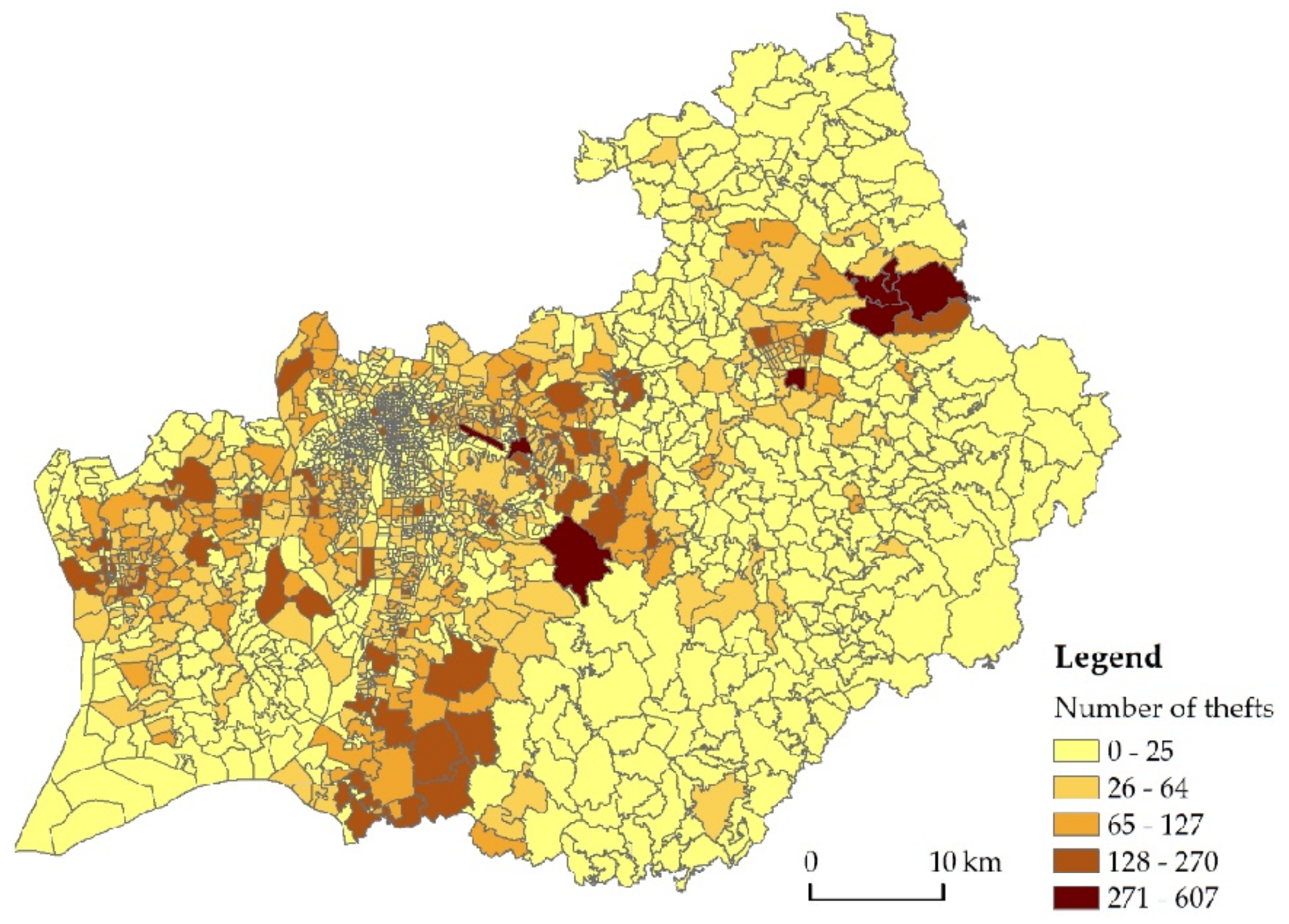
3.1. Spatial Distribution of Theft and Population Type

Figure 1 shows the spatial distribution of thefts. The deeper the color is, the larger the number of thefts will be. The spatial distribution of thefts in ZG City roughly decreases progressively from the center to the periphery and has multiple hot spots. Combined with Figure 2, it can be seen that theft frequently occurs in the middle-income community, the suburban community, the migrant population community, and the affordable housing community; the number of the thefts per 1000 persons can reach 6.647, 5.905, 6.789, and 5.256, respectively, and it is 4.535, 4.239, and 3.567 for the other four kinds of communities (local elderly community, affluent community, college community), indicating saliently spatial heterogeneity in the distribution of thefts. As shown in Table 3, the standard deviation of the number of thefts in each community is 45.384, the mean value is 34.29, and the variance is far larger than the mean value, indicating a saliently discrete phenomenon.

Figure 2 shows the distribution of different categories of communities in ZG city. The clustering result is similar to the result of the classification by Zhou [22]. However, the research classifies areas based on community-scale data instead of town-scale on a smaller scale.

3.2. Negative Binomial Regression Model Results

The negative binomial regression model is shown in

Table 4. Results of Spatial-lag negative binominal regression of ambient population from different communities (N = 1530).

Variables	Coefficient (β)	IRR	Standardized Coefficient
Proportion of migrant population (%)	0.008 ***	1.008	0.189 ***
Proportion of migrant population (%)_lag	0.004	1.004	0.072
Number of offenders	0.054 ***	1.055	0.154 ***
Number of offenders_lag	0.020	1.020	0.030
Distance from the nearest police station (km)	−0.341 ***	0.711	−0.292 ***
Local elderly population	0.004	1.004	0.025
Middle-income population	0.021 ***	1.021	0.161 ***
Affluent population	0.018 ***	1.018	0.089 ***
Affordable housing population	0.010 **	1.010	0.067 **
Migrant population	0.012 ***	1.012	0.357 ***
Suburban population	0.017 ***	1.017	0.257 ***
College population	0.008 ***	1.008	0.107 ***
Local elderly population_lag	−0.014 *	0.986	−0.058 *
Middle-income population_lag	0.018 ***	1.018	0.086 ***
Affluent population_lag	0.030 ***	1.030	0.094 ***
Affordable housing population_lag	0.001	1.001	0.003
Migrant population_lag	−0.003 *	0.997	−0.067 *
Suburban population_lag	−0.006 *	0.994	−0.067 *
College population_lag	0.001	1.001	0.009
AIC	13,001
BIC	13,112.91

*** p < 0.001, ** p < 0.01, * p < 0.05.

. The maximum value of VIF of the model variable is 3.07, indicating no salient collinearity problem.

In terms of control variables, the proportion of the migrant population and number of arrested offenders have a saliently positive influence on theft, that is, the higher the proportion of the migrant population in a community is, or the larger the number of offenders is, the higher the number of thefts will be. It is noted that the spatial lag variable of the arrested offenders and the proportion of the migrant population have no salient influence on theft. The distance from the nearest police station has a negative impact on theft, which means that the closer the community is to the police station, the more the theft that occurs in this area. However, no such spatial lag impact exists. It could be that the police officers’ patrols were not near the station. It could also be that the police station is also located in a high-crime area or that the closer it is to the police station, the more likely residents are to report a crime to the police. This finding is in line with existing studies [3,33].

Different ambient populations were exposed to different opportunity costs, thus having different impacts on crime. Except for the local elderly population, the other categories of ambient populations have a saliently positive influence on theft. Overall, the larger the number of the ambient population is, the higher the number of thefts in the community will be. As shown in Table 4, if the middle-income population, affluent population, affordable housing population, migrant population, suburban population, and college population increase by one unit (1000 person–time) each time, the frequency of the thefts will increase (1.021 − 1) ×100%, (1.018 − 1) × 100%, (1.010 − 1) × 100%, (1.012 − 1) × 100%, (1.017 − 1) × 100%, and (1.008 − 1) × 100%, respectively.

It can be found from the standardized coefficients in Table 4 and the Wald test among different coefficients in

Table 5. Wald test of standardized coefficients for each pair of key variables.

No.	Variables and Standardized Coefficients	X1	X2	X3	X4	X5	X6	X7	X8	X9
X1	Migrant population (0.189)	-
X2	Quantity of criminals (0.0154)	n.s.	-
X3	Distance from the nearest police station (0.292, absolute value of coefficient)	*	*	-
X4	Middle-income population (0.161)	n.s.	n.s.	*	-
X5	Affluent population (0.089)	*	n.s.	***	n.s.	-
X6	Affordable housing population (0.067)	**	n.s.	***	*	n.s.	-
X7	Migrant population (0.357)	*	**	n.s.	***	***	***	-
X8	Suburban population (0.257)	n.s.	n.s.	n.s.	*	***	***	*	-
X9	College population (0.107)	n.s.	n.s.	***	n.s.	n.s.	n.s.	***	***	-

* p < 0.05, ** p < 0.01, *** p < 0.001, n.s. is no significant difference; H0: The coefficient difference between the two variables is 0; the local elderly population has no salient influence and will not be included in the Wald test for analysis.

that different kinds of ambient populations have different influences on theft. The migrant population has the strongest influence, followed by the suburban population and middle-income population, whereas the college population, affluent population and affordable housing population have the weakest influence on the spatial pattern of theft. It is noted that there is no significant difference in influence between the college population and the affluent population, or between the affluent population and the affordable housing population, whereas the college population has a stronger influence compared to the affordable housing population.

In terms of the strength of the influence of the control variables, the standardized coefficient for the distance from the nearest police station is lower than the migrant population, but there is no significant difference; the influences of the proportion of the migrant population and the number of arrested offenders is weaker than the migrant population and the distance from the nearest police station. It can be seen that the main factors influencing the spatial distribution of theft include appropriate criminal targets and guardianship.

In terms of the spatial lag effect, the distribution of the local elderly population, migrant population, and suburban population in adjacent communities will inhibit the number of thefts in the community; the middle-income population and affluent population may lead to an increase in the number of thefts in the adjacent community, whereas the affordable housing population and college population have no significant influence on the number of thefts in the adjacent community. It seems contradictory that the regression coefficient on the migrant population becomes positive as expected, while the coefficient on the spatially lagged migrant population becomes negative. This is because if a community has a large migrant ambient population in the surrounding communities, the offenders will prefer to go to the surrounding communities because there are more potential targets. Then, the community in the center will be less attractive. The same should hold for the suburban population.

4. Discussion

Focusing on one of the three factors (i.e., potential victim) based on the routine activity theory, this research distinguishes the ambient population into different social groups based on their residence and further explores their impacts on theft. While former studies that used the static census and points of interest indirectly reflect the distribution of potential victims, the results show that ambient populations with different types could directly reflect the distribution of potential victims.

Different types of ambient populations have varied influences on theft, which is mainly due to their varied “risk–benefit” features to the offenders. Specifically, migrant population aggregated communities commonly have a high degree of anonymity and weak social control [38,39], therefore leading to a low risk of arrest for the offenders. Moreover, migrant populations are often active in crowded areas, for example, a village in cities, which provides convenience for offenders to steal properties [35,40]. Due to the presented “low risk, high benefit” feature, the migrant population has the strongest influence on the spatial distribution of theft. In contrast, the local elderly population has the significant effect of “eyes on the street” and strong informal social control [7,16]. For theft, the risk is higher than the benefit (“high risk, low income”) to the offenders. The influences of the suburban population and middle-income population on theft ranks only after that of the migrant populations. These kinds of ambient populations have relatively strong informal social control and high benefit for theft due to their wealthier belongings [21,41]. Because of the “middle risk, high benefit” feature, the population still has a large influence on the distribution of theft. The numbers of the college population, affluent population, and the affordable housing population are small, and they have a significantly positive influence on the distribution of theft, but the degree of influence is relatively weak. It is noted that the research only analyzed the relationship between different ambient populations and theft on workdays due to data limitations. During the workday, most college teachers and students attend class (indoor), and the college community is the main activity space. All these have a limited influence on outdoor theft. Although the potential income of theft from the affluent population is high, the security level of the activity space for the population is also high (“high risk, high benefit”) [41]. As a result, the affluent population has a low attraction for the offenders. The affordable housing population features a high degree of education and a strong awareness of precaution, leading to a more balanced risk–return portfolio, which has a certain attraction, but is not strong enough. Overall, thieves follow the rule of “Safety First, Benefit Second” to select the target, which is similar to the result of Xiao et al. [16].

The research has some similarities with the existing literature. For example, the influence of the proportion of the migrant population on theft is also verified as an important index for measuring the social environment of big cities in China; that is, the higher the proportion of the migrant population, the higher the probability of theft in the community will be. The number of local offenders in a community will significantly lead to the increased probability of being stolen from, which further demonstrates that offenders tend to select adjacent regions due to low cost [42]. After controlling for the influences of other variables, the smaller the distance from the nearest police station is, the higher the number of thefts will be, which is consistent with the findings of Song et al. [3] and Mburu et al. [28] but different from the findings of Zhang et al. [43]. It may be related to the distribution of police stations in ZG City, and that the police station is usually located in an area with a dense population.

5. Conclusions

By targeting the shortcoming of the literature regarding ambient populations as homogeneous groups, the innovative point of this research was to find out different influences of various ambient populations on the spatial pattern of theft from the perspective of activity space, which measured potential victims with mobile big data technology and combined the social attributes of mobile users. The theoretical contributions include that, based on the routine activity theory in crime geography, the research further deepens the discussion for potential victims from the perspective of “ambient population + population heterogeneity”. For spatiotemporal behavior, the research discussed the influence of activity space of different populations on theft based on trajectory data, demonstrated the importance of spatiotemporal behavior in crime geography, and expanded the research field of spatiotemporal behavior.

On the application level, the research suggests for the police–geographic department that the focus of crime prevention strategy should shift from the residence space to the activity space. In addition, the department should pay attention to the activity space of the migrant population, suburban population, and middle-income population to implement targeted propaganda and deployment and improve the distribution efficiency of police–geographic resources.

However, the research still has some limitations. First, we only used the mobile phone data from one mobile phone company and only one workday to represent the overall distribution of the ambient population on workdays, which cannot be reflected by the data of the full sample. Although theft on weekends and holidays is not analyzed in this study, whether the results are consistent with the weekday studies is unclear. This issue also occurred in other ambient population and theft-related studies. Second, the importance of time in various crime analyses has been demonstrated in recent years, and the spatial distribution of different social groups changes with time. Therefore, discussions are also required on the time difference in the influence of different populations on theft. Finally, the research provides the attributes of the community to each mobile user, but heterogeneity also exists among populations in the community, and existing big data cannot be used to accurately determine the user attribute of each individual. Therefore, the accuracy of population portrayal and spatial granularity therein still need to be improved in future studies.

References

1. Cohen, L.E.; Felson, M. Social change and crime rate trends: A routine activity approach. Am. Sociol Rev. 1979, 44, 588–608. [Google Scholar] [CrossRef]
2. Brantingham, P.L.; Brantingham, P.J. Nodes, paths and edges: Considerations on the complexity of crime and the physical environment. J. Environ. Psychol. 1993, 13, 3–28. [Google Scholar] [CrossRef]
3. Song, G.; Liu, L.; Bernasco, W.; Xiao, L.; Zhou, S.; Liao, W. Testing Indicators of Risk Populations for Theft from the Person across Space and Time: The Significance of Mobility and Outdoor Activity. Ann. Am. Assoc. Geogr. 2018, 108, 1370–1388. [Google Scholar] [CrossRef]
4. Hipp, J.R. General Theory of Spatial Crime Patterns. Criminology 2016, 54, 653–679. [Google Scholar] [CrossRef] [Green Version]
5. Crols, T.; Malleson, N. Quantifying the Ambient Population Using Hourly Population Footfall Data and An Agent-based Model of Daily Mobility. Geoinformatica 2019, 23, 201–220. [Google Scholar] [CrossRef] [Green Version]
6. Melo, S.N.D.; Andresen, M.A.; Matias, L.F. Geography of crime in a Brazilian context: An application of social disorganization theory. Urban Geogr. 2017, 38, 1550–1572. [Google Scholar] [CrossRef]
7. Song, G.; Liu, L.; Bernasco, W.; Zhou, S.; Xiao, L.; Long, D. Theft from the person in urban China: Assessing the diurnal effects of opportunity and social ecology. Habitat. Int. 2018, 78, 13–20. [Google Scholar] [CrossRef]
8. Xu, C.; Yang, Y.; Song, G.; Liu, L.; Lan, M.; Chen, X. The impact of civil registration-based demographic heterogeneity on community thefts. Habitat. Int. 2022, 129, 102673. [Google Scholar] [CrossRef]
9. Zeng, M.; Mao, Y.; Wang, C. The relationship between street environment and street crime: A case study of Pudong New Area, Shanghai, China. Cities 2021, 112, 103143. [Google Scholar] [CrossRef]
10. Boggs, S.L. Urban Crime Patterns. Am. Sociol Rev. 1965, 30, 899–908. [Google Scholar] [CrossRef]
11. Boivin, R.; Felson, M. Crimes by Visitors Versus Crimes by Residents: The Influence of Visitor Inflows. J. Quant. Criminol. 2018, 34, 465–480. [Google Scholar] [CrossRef]
12. Hanaoka, K. New insights on relationships between street crimes and ambient population: Use of hourly population data estimated from mobile phone users’ locations. Environ. Plan. B Urban Anal. City Sci. 2016, 45, 295–311. [Google Scholar] [CrossRef]
13. Malleson, N.; Andresen, M.A. The impact of using social media data in crime rate calculations: Shifting hot spots and changing spatial patterns. Cartogr. Geogr. Inf. Sci. 2015, 42, 112–121. [Google Scholar] [CrossRef]
14. Malleson, N.; Andresen, M.A. Exploring the impact of ambient population measures on London crime hotspots. J. Crim. Just. 2016, 46, 52–63. [Google Scholar] [CrossRef] [Green Version]
15. Cornish, D.B.; Clarke, R.V. Understanding crime displacement: An Application of Rational Choice Theory. Criminology 1987, 25, 933–948. [Google Scholar] [CrossRef]
16. Xiao, L.; Liu, L.; Song, G.; Zhou, S.; Long, D.; Feng, J. Impacts of community environment on residential burglary based on rational choice theory. Geogr. Res. Aust. 2017, 36, 2479–2491. [Google Scholar]
17. Shen, Y.; Chai, Y. Daily Activity Space of Suburban Mega-community Residents in Beijing Based on GPS Data. Acta. Geographica. Sinica. 2013, 68, 506–516. [Google Scholar]
18. Valente, R.; Medina-Ariza, J. Mobility, Nonstationary Density, and Robbery Distribution in the Tourist Metropolis. Eur. J. Crim. Policy Res. 2022. [Google Scholar] [CrossRef]
19. Song, G.; Zhang, Y.; Bernasco, W.; Cai, L.; Liu, L.; Qin, B.; Chen, P. Residents, Employees and Visitors: Effects of Three Types of Ambient Population on Theft on Weekdays and Weekends in Beijing, China. J. Quant. Criminol. 2021. [Google Scholar] [CrossRef]
20. Hirschfield, A.; Birkin, M.; Brunsdon, C.; Malleson, N.; Newton, A. How Places Influence Crime: The Impact of Surrounding Areas on Neighbourhood Burglary Rates in a British City. Urban Stud. 2014, 51, 1057–1072. [Google Scholar] [CrossRef] [Green Version]
21. Xiao, L.; Ruiter, S.; Liu, L.; Song, G.; Zhou, S. Burglars blocked by barriers? The impact of physical and social barriers on residential burglars’ target location choices in China. Comput. Environ. Urban Syst. 2021, 86, 101582. [Google Scholar] [CrossRef]
22. Zhou, C.; Hu, J.; Tong, X.; Bian, Y. The Socio-Spatial Structure of Guangzhou and Its Evolution. Acta. Geographica. Sinica. 2016, 71, 1010–1024. [Google Scholar]
23. Lammers, M.; Menting, B.; Ruiter, S.; Bernasco, W. Biting Once, Twice: The Influence of prior on subsequent crime location choice. Criminology 2015, 53, 309–329. [Google Scholar] [CrossRef]
24. Townsley, M.; Birks, D.; Bernasco, W.; Ruiter, S.; Johnson, S.D.; White, G.; Baum, S. Burglar Target Selection: A Cross-national Comparison. J. Res. Crime. Delinq. 2014, 52, 3–31. [Google Scholar] [CrossRef] [Green Version]
25. Townsley, M.; Birks, D.; Ruiter, S.; Bernasco, W.; White, G. Target Selection Models with Preference Variation Between Offenders. J. Quant. Criminol. 2016, 32, 283–304. [Google Scholar] [CrossRef] [Green Version]
26. Bernasco, W.; Johnson, S.D.; Ruiter, S. Learning Where to Offend: Effects of Past on Future Burglary Locations. Appl. Geogr. 2015, 60, 120–129. [Google Scholar] [CrossRef] [Green Version]
27. Bernasco, W.; Block, R.; Ruiter, S. Go Where the Money Is: Modeling Street Robbers’ Location Choices. J. Econ. Geogr. 2013, 13, 119–143. [Google Scholar] [CrossRef] [Green Version]
28. Mburu, L.W.; Helbich, M. Crime Risk Estimation with a Commuter-Harmonized Ambient Population. Ann. Am. Assoc. Geogr. 2016, 106, 804–818. [Google Scholar] [CrossRef]
29. Osgood, D.W. Poisson-Based Regression Analysis of Aggregate Crime Rates. J. Quant. Criminol. 2000, 16, 21–43. [Google Scholar] [CrossRef]
30. Zhou, S.; Deng, L. Spatio-temporal Pattern of Residents’ Daily Activities Based on T-GIS: A Case Study in Guangzhou, China. Acta. Geographica. Sinica. 2010, 65, 1454–1463. [Google Scholar]
31. Zhou, S.; Deng, L. Spatio-temporal Agglomeration of Low-income people’s Daily Activity and Related Factors: A Case Study of Guangzhou. City Plan. Rev. 2017, 41, 17–25. [Google Scholar]
32. Liu, L.; Feng, J.; Ren, F.; Xiao, L. Examining the Relationship Between Neighborhood Environment and Residential Locations of Juvenile and Adult Migrant Burglars in China. Cities 2018, 82, 10–18. [Google Scholar] [CrossRef]
33. Helbich, M.; Jokar Arsanjani, J. Spatial Eigenvector Filtering for Spatiotemporal Crime Mapping and Spatial Crime Analysis. Cartogr. Geogr. Inf. Sci. 2015, 42, 134–148. [Google Scholar] [CrossRef]
34. Zhang, L.; Messner, S.F.; Liu, J. A Multilevel Analysis of the Risk of Household Burglary in the City of Tianjin, China. Br. J. Criminol. 2007, 47, 918–937. [Google Scholar] [CrossRef]
35. Chen, J.; Liu, L.; Zhou, S.; Xiao, L.; Jiang, C. Spatial Variation Relationship between Floating Population and Residential Burglary: A Case Study from ZG, China. Isprs. Int. J. Geo. Inf. 2017, 6, 246. [Google Scholar] [CrossRef]
36. Berk, R.; MacDonald, J.M. Overdispersion and Poisson Regression. J. Quant. Criminol. 2008, 24, 269–284. [Google Scholar] [CrossRef]
37. Land, K.C.; McCall, P.L.; Nagin, D.S. A Comparison of Poisson, Negative Binomial, and Semiparametric Mixed Poisson Regression Models: With Empirical Applications to Criminal Careers Data. Sociol Method. Res. 1996, 24, 387–442. [Google Scholar] [CrossRef]
38. Li, S. Housing Tenure and Residential Mobility In Urban China: A Study of Commodity Housing Development in Beijing and Guangzhou. Urban Aff. Rev. 2003, 38, 510–534. [Google Scholar] [CrossRef]
39. Liu, G. A Behavioral Model of Work-Trip Mode Choice in Shanghai. China Econ. Rev. 2007, 18, 456–476. [Google Scholar] [CrossRef] [Green Version]
40. Lin, Y.; de Meulder, B.; Wang, S. Understanding the ‘Village in the City’ in Guangzhou: Economic Integration and Development Issue and their Implications for the Urban Migrant. Urban Stud. 2011, 48, 3583–3598. [Google Scholar] [CrossRef]
41. Vandeviver, C.; Neutens, T.; van Daele, S.; Geurts, D.; Vander Beken, T. A discrete spatial choice model of burglary target selection at the house-level. Appl. Geogr. 2015, 64, 24–34. [Google Scholar] [CrossRef] [Green Version]
42. Bernasco, W. Modeling Micro-Level Crime Location Choice: Application of the Discrete Choice Framework to Crime at Places. J. Quant. Criminol. 2010, 26, 113–138. [Google Scholar] [CrossRef]
43. Zhang, Y.; Zhu, C.; Qin, B. Spatial distribution of crime number and harm and the influence of the built environment: A longitudinal research on criminal cases in Beijing. Prog. Geogr. 2019, 38, 1876–1889. [Google Scholar] [CrossRef]
Figure 1. The spatial distribution of the number of thefts.
Ijgi 11 00615 g001
Figure 2. The distribution of different categories of communities in ZG city.
Ijgi 11 00615 g002