Abstract
Several studies have worked on co-clustering analysis of spatio-temporal data. However, most of them search for co-clusters with similar values and are unable to identify co-clusters with coherent trends, defined as exhibiting similar tendencies in the attributes. In this study, we present the Bregman co-clustering algorithm with minimum sum-squared residue (BCC_MSSR), which uses the residue to quantify coherent trends and enables the identification of co-clusters with coherent trends in geo-referenced time series. Dutch monthly temperatures over 20 years at 28 stations were used as the case study dataset. Station-clusters, month-clusters, and co-clusters in the BCC_MSSR results were showed and compared with co-clusters of similar values. A total of 112 co-clusters with different temperature variations were identified in the Results, and 16 representative co-clusters were illustrated, and seven types of coherent temperature trends were summarized: (1) increasing; (2) decreasing; (3) first increasing and then decreasing; (4) first decreasing and then increasing; (5) first increasing, then decreasing, and finally increasing; (6) first decreasing, then increasing, and finally decreasing; and (7) first decreasing, then increasing, decreasing, and finally increasing. Comparisons with co-clusters of similar values show that BCC_MSSR explored coherent spatio-temporal patterns in regions and certain time periods. However, the selection of the suitable co-clustering methods depends on the objective of specific tasks.
1. Introduction
Thanks to the advancement of earth observation and model simulation systems, unprecedented amounts of spatio-temporal data with various resolutions have been accumulated [1,2]. On one hand, these massive amounts of data provide opportunities to investigate complex patterns and knowledge to help decision-making [3]; on the other hand, how to extract patterns from these data becomes a challenging issue [4]. As one of the most important data mining tasks, clustering methods group data elements into clusters by identifying similar ones and separating dissimilar ones, thus helping to extract underlying patterns in the data [5,6,7].
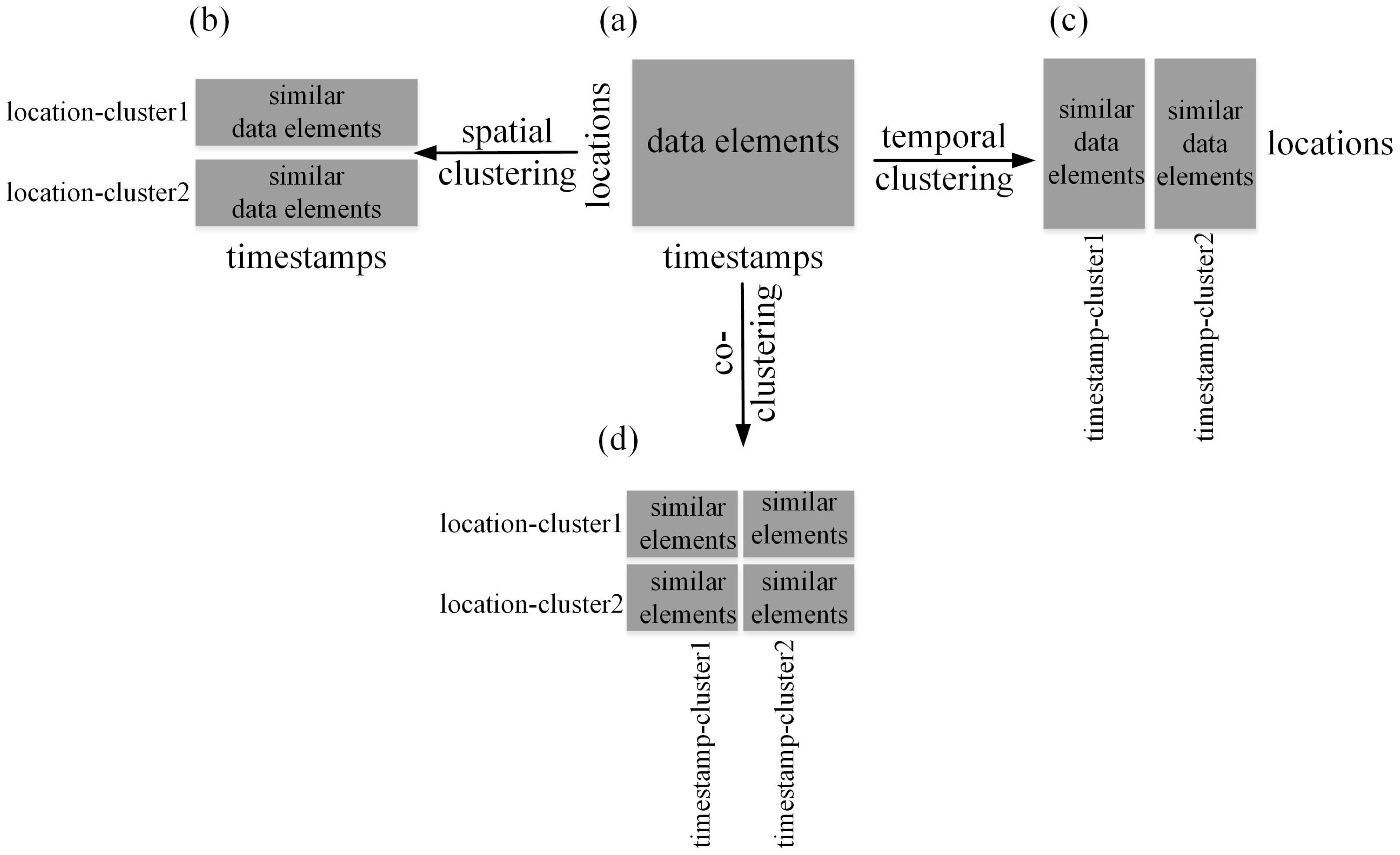
There have been many studies on analyzing patterns in spatio-temporal data using clustering methods [8]. Most studies applied traditional clustering methods, also named one-way clustering methods, which analyze either spatial or temporal patterns in the data and are thus called spatial clustering or temporal clustering. In particular, spatial clustering methods analyze data along the spatial dimension and partition similar data elements along all the timestamps into clusters of locations (Figure 1a,b). For example, Andrienko et al. [9] used a self-organizing map (SOM) as a one-way clustering method to identify spatial clusters of similar temporal distributions in city traffic data. Hagenauer and Helbich [10] proposed hierarchical spatio-temporal SOM (HSTSOM), which analyzed spatial and temporal patterns separately in the layers to search for clusters in socio-economic data. Liu et al. [11] applied k-means clustering method to identify spatial clusters of states with similar time series of spatial autocorrelation curves to examine the effect of policies on COVID-19 transmission. Temporal clustering methods analyze the data along the temporal dimension and group similar data elements along all the locations into clusters of timestamps (Figure 1a,c). For instance, Ahas et al. [12] grouped years with similar rhythm of human activities by clustering analysis to differentiate urban and rural landscapes. Wu et al. [13] identified years with similar temperature variations along all stations in the Netherlands to explore temporal varying behavior in Dutch weather data.
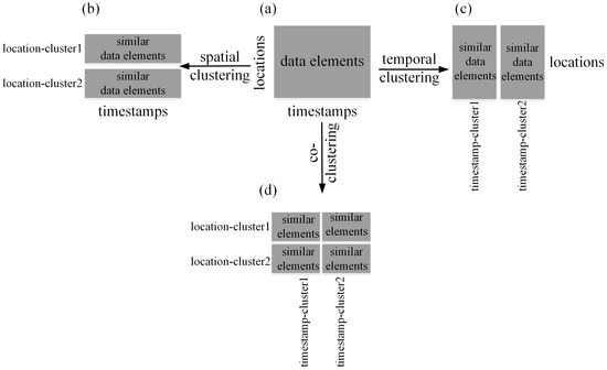
Figure 1.
One-way clustering (a–c), co-clustering (a,d).
Recently, co-clustering analysis of spatio-temporal data has attracted the attention of researchers in geo-field. Unlike one-way clustering, co-clustering methods (Figure 1a,d) analyze the data from both spatial and temporal aspects simultaneously, and partition similar data elements along both dimensions into clusters of locations and timestamps [8]. Consequently, they are capable of discovering both spatial and temporal patterns in the data simultaneously. Wu et al. [14] applied the co-clustering method to analyze temperature patterns along both spatial and temporal dimensions in Dutch temperature series. Wu et al. [15] and Wu et al. [16] used the co-clustering method to explore patterns of both spatial and temporal differentiations in long-term spring phenology in Europe and China, respectively. Ullah et al. [17] detected potential space-time disease clusters in annual and monthly malaria series in Pakistan by using co-clustering analysis. Andreo et al. [18] used the co-clustering method to identify spatio-temporal clusters of favorable conditions for West Nile emergence and maintenance in Greece. Liu et al. [19] applied the co-clustering method to Manhattan Taxi data to discover mobility patterns in both spatial and temporal dimensions.
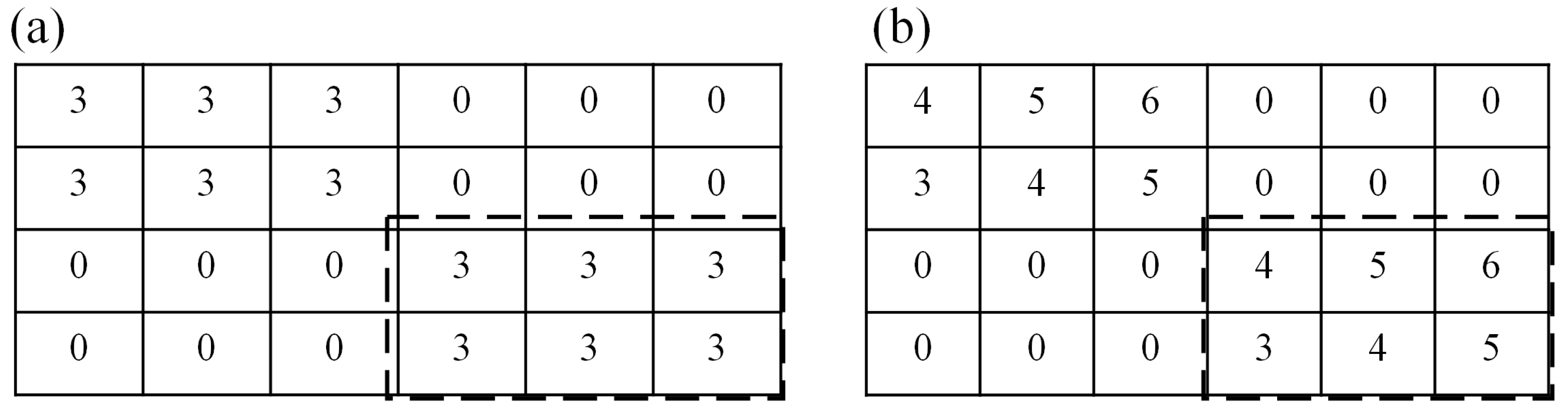
Even though those aforementioned co-clustering methods have analyzed the data from both spatial and temporal aspects, they are only capable of identifying co-clusters with similar values. For instance, in the toy datasets in Figure 2 where rows indicate locations, columns indicate timestamps, and values indicate temperature, the similar values in the thick dashed rectangle in Figure 2a can be identified by those co-clustering methods as one co-cluster. However, they may fail to discover co-clusters with coherent trends, where subsets of timestamps have similar varying behavior only under subsets of locations, e.g., the values in the thick dashed line in Figure 2b. Here, the coherent trend is defined as exhibiting similar tendencies in the values of the attribute(s) [20,21]. The identification of co-clusters with coherent trends is important to help explore patterns in many applications. Take climatology for instance, the study of temperature trends has attracted attention of researchers because it was found to have impacts on crop yields, population dynamics of insects, and even high deaths of elderly people with chronic disease [22,23,24,25]. Besides, crime analysis could also benefit from such a co-clustering method, in that the identified similar trends of occurrences at various locations would help the police to investigate the movement of gangsters and take relevant measures efficiently [26]. Thus, the use of a co-clustering method that is able to identify co-clusters with similar varying behavior in spatio-temporal data is necessary.
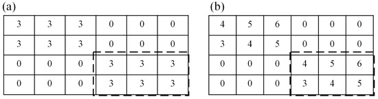
Figure 2.
Toy datasets with co-cluster examples as similar values (a) and similar trends (b) surrounded by thick dashed rectangles.
Unlike the aforementioned co-clustering methods that seek for high similarity of values in the co-cluster, the co-clustering methods for coherent trends aim at high score of coherence in the co-cluster [27]. As stated by Eisen et al. [20], the coherent trend of measurement series can be calculated by various methods, e.g., Euclidean distances, correlations coefficient etc. Cheng and Church [28] introduced the residue as the distance measure to quantify the coherent trend for co-clusters. The residue is termed as the differences between each element in the co-cluster and the matching row mean as well as column mean [29]. Take the toy dataset in Figure 2b for example, the clustering assignment {1122} for rows and {111222} for columns would be preferred, considering the row and column distributions of the dataset. With such assignment, the values in the thick dashed rectangle in Figure 2b is partitioned as one co-cluster, and the residue of elements in the co-cluster equals to zero.
Several studies have worked on co-clustering methods with coherent trends for exploring coherent patterns, especially in the field of microarray analysis. As aforementioned, Cheng and Church [28] first proposed the minimum sum-squared residue co-clustering algorithm (MSSRCC) to search for co-regulation patterns in expression data. Cho and Dhillon [30] applied MSSRCC with different strategies, e.g., incremental local search, to search for coherent co-clusters in both synthetic and several real gene expression datasets. Yang et al. [31] introduced a co-clustering algorithm called flexible overlapped biclustering that yields all overlapping co-clusters whose mean residues are smaller than a predefined value to explore coherent patterns in gene expression data. Kluger et al. [32] proposed a spectral co-clustering algorithm which computes a singular vector of normalized gene expression data, projects data onto the topmost vectors, and then applies normalized cuts. Rathipriya et al. [33] developed a binary particle swarm optimization-based co-clustering algorithm which combines swarm intelligent technique and co-clustering to discover coherent relationships between web users and web pages.
The objective of this study is, thus, to apply a co-clustering method to spatio-temporal data, which enables the identification of spatio-temporal co-clusters with coherent trends. Here, we focus on geo-referenced time series, one important type of spatio-temporal data, which are usually recorded at stationary locations and timestamps with uniform intervals. Dutch monthly temperature series are used to illustrate the co-clustering method. As far as we know, none of previous studies identified co-clusters with coherent trends in spatio-temporal data. The novelty of this research lies in the following three aspects: (1) A co-clustering algorithm that enables the identification of co-clusters with coherent trends is introduced to analyze Dutch meteorological temperature series; (2) 112 co-clusters with different temperature variations were identified by the co-clustering algorithm, and seven types of coherent temperature trends were summarized. (3) Comparisons with co-clusters of similar values reveal differences between these two types of methods.
The rest of this paper is organized as follows. Section 2 describes the Dutch temperature dataset and the specific co-clustering algorithm used in this study. Next, Section 3 presents results of the co-clustering analysis of Dutch temperature series, and discusses the differences between co-clusters with similar values and coherent trends. Finally, Section 4 draws conclusions.
2. Data and Methods
This section first presents the dataset and the study area used to illustrate this study. Afterwards, the specific co-clustering algorithm, named Bregman co-clustering algorithm, with minimum sum-squared residue is described in detail.
2.1. Data
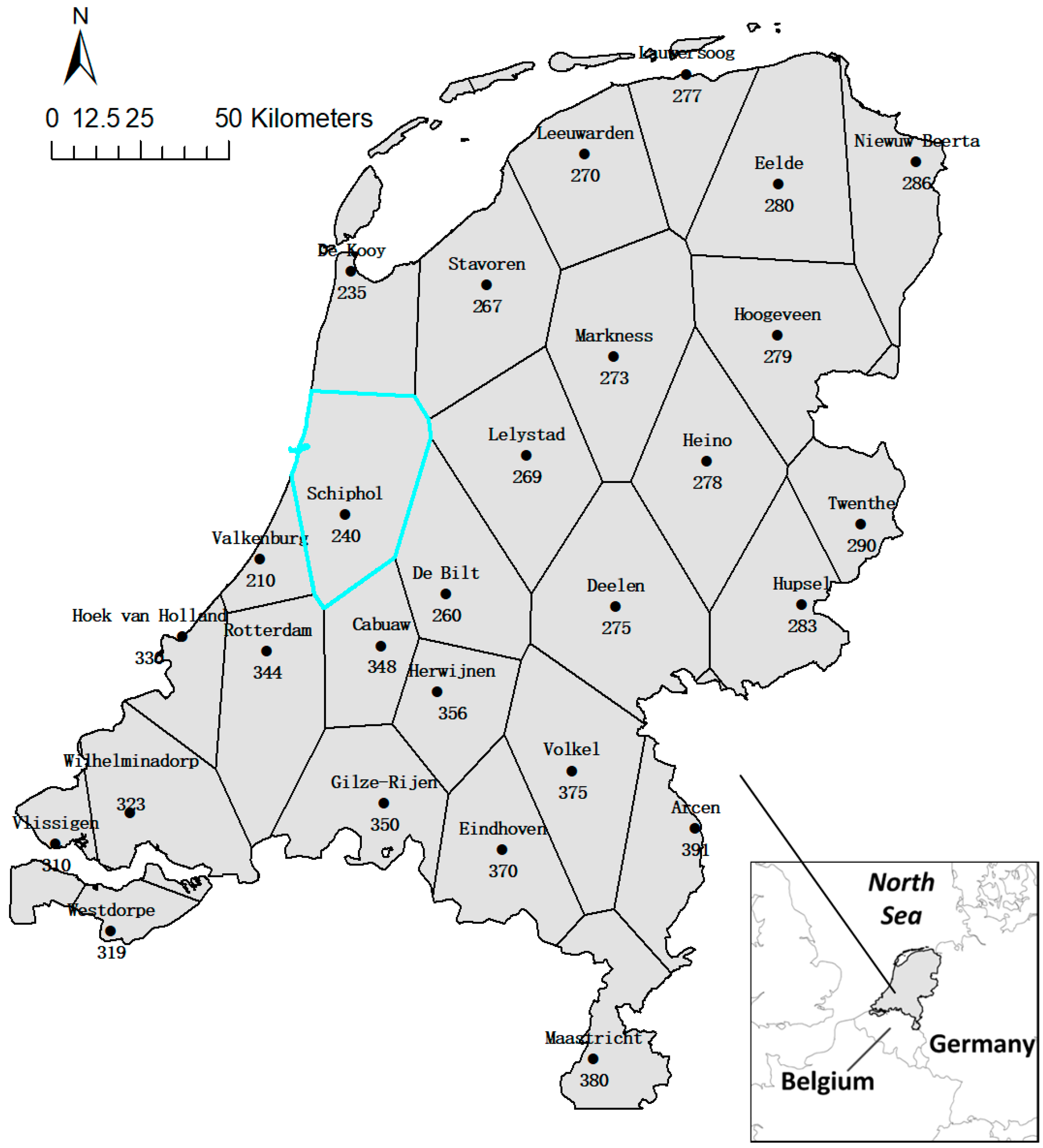
Monthly temperatures from January 1992 to December of 2011 at 28 meteorological stations in the Netherlands were used as the case study dataset to illustrate the identification of co-clusters with coherent trends. The original daily temperature data was freely available at the website of the Royal Netherlands Meteorological Institute (KNMI, https://dataplatform.knmi.nl/ (accessed on 14 February 2022)), which were then averaged to generate the monthly average temperatures. The Thiessen polygons map (Figure 3) was created using the stations’ coordinates to define the area that each station had influence on, e.g., the highlighted polygon indicating the influenced area by the station Schiphol (240).
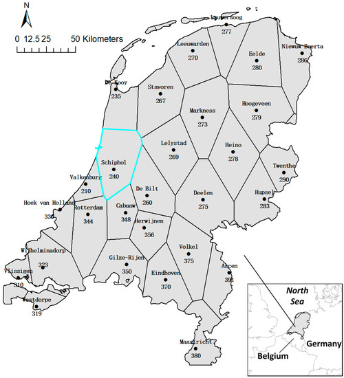
Figure 3.
The study area and Thiessen polygons map indicating influenced area by stations.
The Netherlands were chosen as the study area for its location. With the North Sea as its neighbor in the north and west, as well as Belgium and Germany as neighbors in the south and east, respectively, the weather of the Netherlands is influenced by the moderate marine climate in the west and the continental climate in the east. As a result, temperatures gradually change from the southwest to the northeast of this country.
2.2. Bregman Co-Clustering Algorithm with Minimum Sum-Squared Residue (BCC_MSSR)
Unlike co-clustering methods that identify co-clusters with similar values, co-clustering methods for exploring local coherent varying behavior search for co-clusters with similar trends. By mapping locations to location-clusters and timestamps to timestamp-clusters, they result in co-clusters within each, of which the tendencies of the attribute(s) were similar. The MSSRCC is used in this study because its authenticity was empirically improved in several datasets and termed as Bregman co-clustering algorithm with minimum sum-squared residue (BCC_MSSR) following the work of [27]. Unlike the information divergence used in the Bregman block average co-clustering algorithm with I-divergence (BBAC_I) that identified co-clusters with similar values, the residue was used as the distance measure of coherent trends in the co-clusters for BCC_MSSR, as mentioned earlier. The sum-squared residue was then defined as the sum of squared variances of any element in the co-cluster and the matching row mean and column mean, which was used to construct the objective function before and after mapping. The optimization of the co-clustering issue could be regarded as the problem of minimizing the total squared residue.
BCC_MSSR algorithm enables the identification of co-clusters with coherent trends in any real valued data matrix. The Dutch monthly temperature series used in the case study can be organized as a co-occurrence matrix between the two variables: stations (S) taking values in stations sets {1, 2, …, z}, and months (M) taking values in all months. In other words, the temperature series can be formalized as the data matrix . Suppose the stations and months are mapped to k and l, station-clusters and month-clusters, respectively, in the co-lustering analysis. Then, the data matrix after co-clustering is , with taking values in the station-cluster sets {1, 2, …, k} and taking values in the month-clusters sets {1, 2, …, l}.
Suppose that I and J indicate the set of indices of locations in a location-cluster and the set of indices of timestamps in a timestamp-cluster, respectively. The residue of a specific element, , in a co-cluster is calculated as
where indicates the mean of elements in station i whose month indices fall into J, indicates the mean of elements in month j whose station indices fall into I, and indicates the mean of all elements in that co-cluster. The residue matrix H can be represented as , where R and C are rows (stations) and columns (months) cluster indicator matrices with the size z × k and n × l respectively, and is the transposed matrix of R.
Then, the objective function of BCC_MSSR is represented as the sum-squared residue of elements before and after co-clustering:
where denotes the norm of a matrix, e.g., . Then, the co-clustering problem becomes the minimization issue. To minimize the objective function to obtain the optimal co-clustering results, BCC_MSSR was designed with an iterative process. The optimization procedure of this co-clustering algorithm is described in following steps (Figure 4):
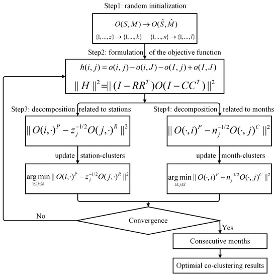
Figure 4.
Workflow of Bregman co-clustering algorithm with minimum sum-squared residue.
Step 1: Random initialization. Station-clusters and month-clusters were randomly mapped to station-clusters and month-clusters, which generated the initial R and C.
Step 2: Calculation of the residue and the objective function. The residue of each element as well as the sum-squared residue of elements before and after mapping were calculated, which can be further represented as
Step 3: Update mapping from stations to station-clusters. The Equation (3) was firstly decomposed to sum-squared residue related to rows (stations) [30]:
where , and denote the ith row (station) in . Then, the new station-clusters membership can be updated by minimizing the Equation (4):
Step 4: Update mapping from months to month-clusters. Equation (3) could be also decomposed to sum-squared residue related to columns (months):
Step 5: Re-calculation of the residue and objective function. The residue and the objective function were recalculated using the updated station-clusters and month-clusters. Once the objective function achieved the convergence with the change of the function below a threshold, the optimal station-clusters and month-clusters were yielded. Otherwise, repeat steps 3–5 until convergence. Since trends in geo-referenced time series data require consecutive timestamps, such a constraint was added for the month-clusters in the co-clustering results by selecting those with consecutive months. Finally, the optimal co-clustering results were yielded.
Both Banerjee, Dhillon, Ghosh, Merugu, and Modha [27], and Cho and Dhillon [30] proved that the objective function in Equation (3) can achieve convergence as it was monotonically minimized with iterations. However, since the clustering algorithm was locally optimized, the whole optimization procedure was typically repeated with multiple runs to obtain the optimal co-clustering results. Finally, it is worth mentioning that MATLAB version R2019b was used for implementing the co-clustering algorithm in this study, and the codes are available upon reasonable request.
3. Results and Discussion
The monthly temperature data with the size of 28 (stations) × 240 (months) was analyzed by BCC_MSSR to identify spatio-temporal co-clusters with coherent trends. The number of station-clusters and month-clusters were optimized using the silhouette method and k-means. The silhouette method was used because it can produce clustering results that have high correlation with experts’ judgement [34,35]. Two to fifteen with an interval of one were used as the candidate numbers of station-cluster and month-cluster. With the number of four for both station-cluster and month-cluster, the silhouette method gave 0.6492 and 0.7252 as the highest values. Thus, four was selected as the optimal number for both station-clusters and month-clusters.
After the co-clustering analysis, the 28 stations and 240 months were mapped to four station-clusters and four month-clusters, respectively, which are displayed using small multiples and diamond charts in Figure 5 and Figure 6. Co-clusters were intersected by each station-cluster and each set of consecutive months in month-clusters under this circumstance. Doe to the local/global minimum issue existing in all clustering algorithms [15], we focus on some co-clusters that frequently appear in the BCC_MSSR results. Those co-clusters are displayed using the heatmaps and line charts in Figure 7.
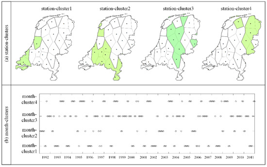
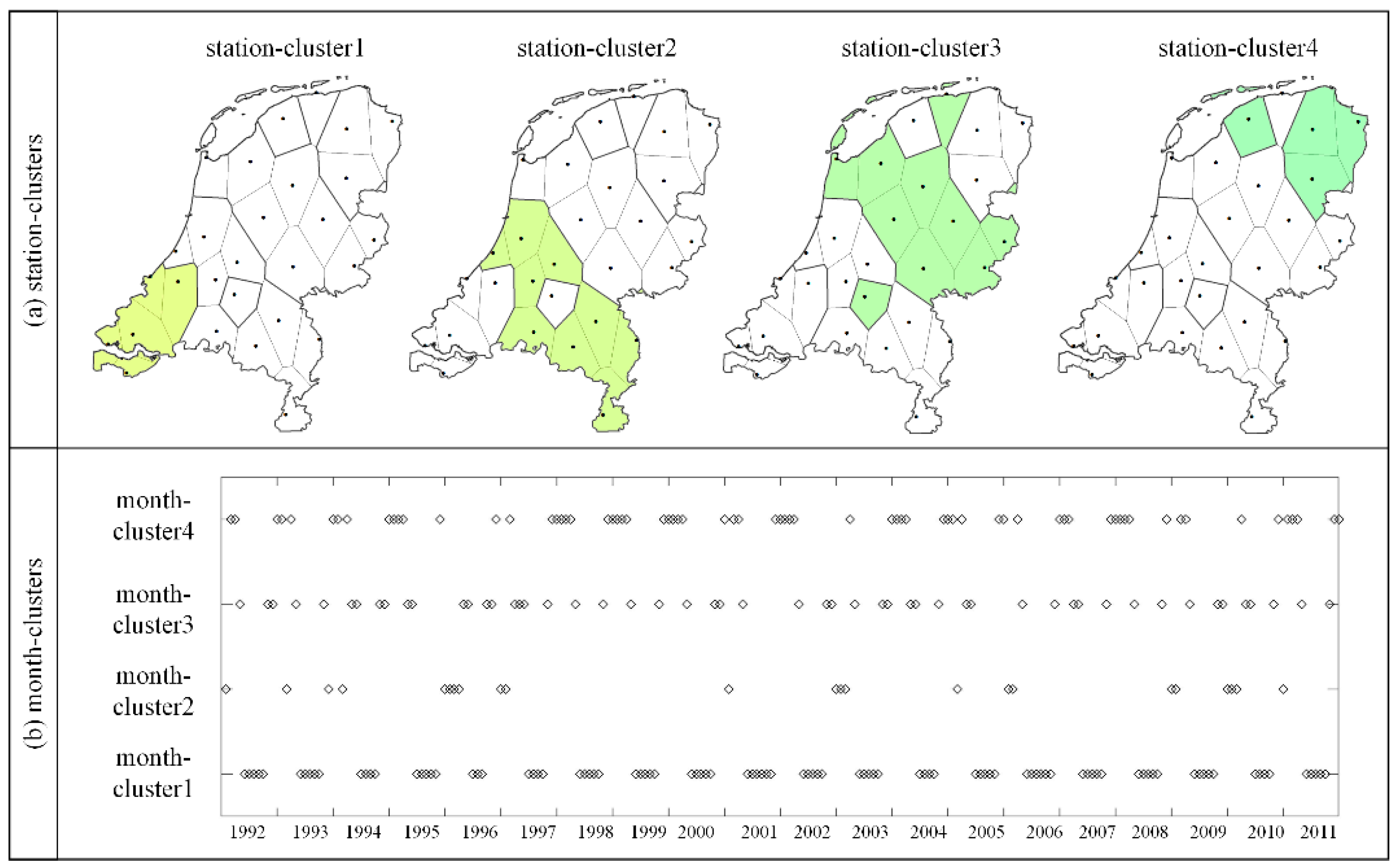
Figure 5.
Station-clusters (a) and month-clusters (b) in the co-clustering results.

Figure 6.
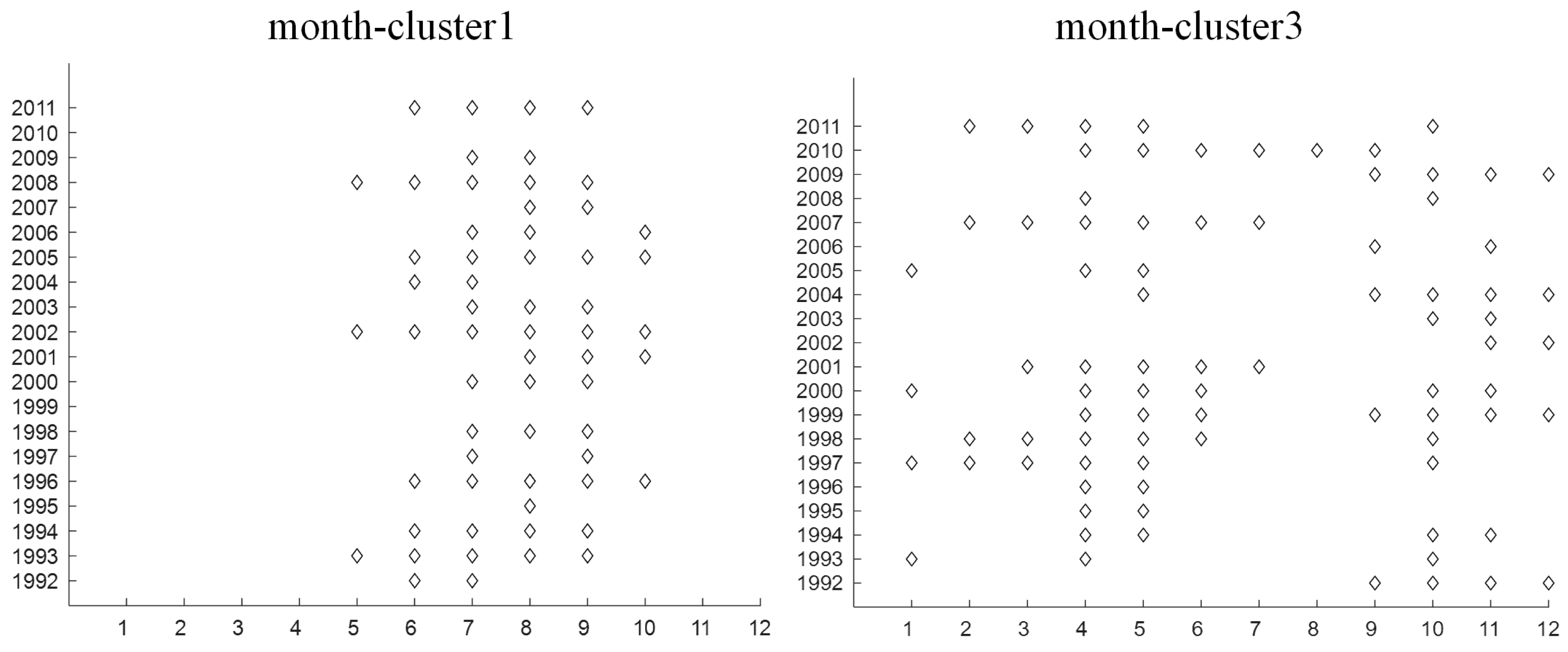
Temporal distribution of months in month-cluster1 and month-cluster3 over 240 months in 20 years.

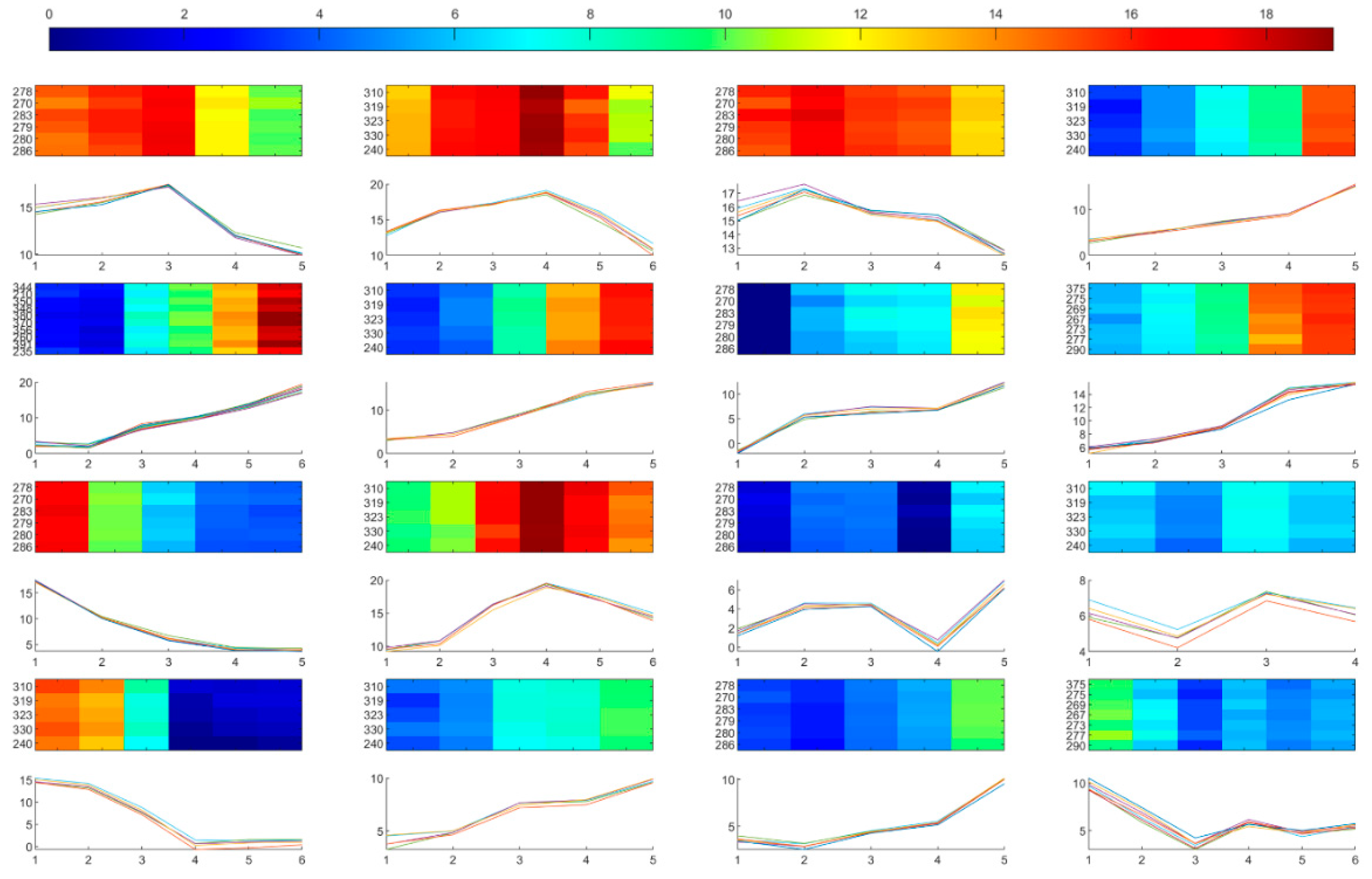
Figure 7.
The 16 representative co-clusters with different temperatures trends among them and similar trends within each co-cluster.
3.1. Spatio-Temporal Co-Clusters with Coherent Trends
Figure 5a shows the spatial distribution of four station-clusters over the Netherlands with colors. The whole country was divided into four regions from the southwest to northeast. Unlike the increasing temperature patterns found in the results of previous co-clustering analysis of Dutch temperature series [14,36], there were no increasing or decreasing temperature patterns in these four regions in this study. It is because these four station-clusters were partitioned based on temperature variations, and it is possible that two stations with similar temperature variations have different temperature values. Stations within each region have similar temperature variations, e.g., Schipol (240), Hoek van Holland (330), Wilhelminadorp (323), Vlissigen (310), and Westdorpe (319) in station-cluster1. Most stations in each station-cluster were adjacent, except Schipol (240) in station-cluster1, De Kooy (235) in station-cluster2, Twenthe (290) in station-cluster3, and Leeuwarden (270) in station-cluster4.
The temporal distribution of elements in each of the month-clusters over 240 months is displayed in Figure 5b. Because of the assignment of BCC_MSSR, the months were not always consecutive in month-clusters. Due to the requirement of consecutive timestamps, we selected those months that were consecutive for at least four timestamps in each month-cluster as potential months to construct co-clusters with similar temperature variations. To further explain the situation, the temporal distribution of months in month-cluster1 and month-cluster3 over 240 months in 20 years are displayed in Figure 6, whereby the x-axis is 12 months and the y-axis is 20 years. We can see that months in month-cluster1 were mostly distributed around the summer. Even though the lengths of consecutive months in month-cluster1 were different, they still had similar temperature variations, e.g., May to September 2008 and May to October 2002. It is also worth mentioning that consecutive months at the two years of transition were also considered as potential months, e.g., September 2004 to January 2005. According to the criteria for potential months to construct co-clusters, 28 sets of consecutive months were selected. Consequently, 112 co-clusters (28 × 4 station-clusters) with similar temperature variations were generated. Due to limited space, 16 representative co-clusters are displayed (Figure 7) and similar co-clusters are described in the text.
Figure 7 shows those 16 representative co-clusters with different temperature trends among them. The trends were similar within each co-cluster. One heatmap and one line chart were used to display each co-cluster: the heatmap on the top provides the direct view of the co-cluster, with the x-axis indicating the number of consecutive months and y-axis indicating the involved stations; while the line chart below shows the coherent temperature trends of the co-cluster, with the y-axis indicating temperature values.
Overall, there are mainly seven types of coherent temperature trends in the representative co-clusters, ranked by the degree of complexity, as follows: (1) increasing; (2) decreasing; (3) first increasing and then decreasing; (4) first decreasing and then increasing; (5) first increasing, then decreasing, and finally increasing; (6) first decreasing, then increasing, and finally decreasing; (7) first decreasing, then increasing, decreasing, andfinally increasing. As displayed in Figure 7, the fourth to eighth co-clusters all exhibit increasing temperature trends, even with various ranges of temperatures and differences in increasing speed. The involved stations were those stations in the southwestern part of the Netherlands, and the involved months were January to May 1992. Such increasing temperature trends in winter and early spring might cause earlier onset and the extension of the growing season in provinces nearby the coastline [37]. Co-clusters with similar temperature trends were intersections of station-cluster1, February to June 2006, and February to May 2011. In the eighth co-cluster, we can see that the speed is constant at first, then it accelerated, and finally decelerated. The involved stations were those in the center-northeastern part of the country, and the involved months were February to June 1998. Co-clusters with similar coherent trends were intersections of station-cluster3 in the center-northeastern part, February to July 2007, and February to May 2011. The co-cluster showing decreasing temperature trends was the ninth one, with smooth declining curves. The involved stations were those stations in the northeastern part of the country, and the involved months were September 1999 to January 2000. Co-clusters with similar decreasing trends were intersections of station-cluster4, September 1991 to January 1992, and September 2003 to February 2004. The decreasing temperature trend in the winter after the heat wave in the summer of 2003 might lead to the another increase in the premature deaths in the northern provinces [37,38].
Several co-clusters exhibit first increasing and then decreasing temperature trends in Figure 7, i.e., first to third and tenth ones, with different ranges of temperatures. The first to third co-clusters start with relatively high temperature, then increase, and finally decrease. Even with these similarities, they are still different in the turning timestamps for decreasing and also the speeds of increasing and decreasing. The involved stations of first and third co-clusters were those stations in the northeastern part of the country, and the involved months were June to October 1996 and May to October 2005, respectively. The involved stations of the second co-cluster were stations in the southwest, and the involved months were May to October 2002. Co-clusters exhibiting similar temperature trends were stations in the northeast, May to October 1993, June to October 1994, and May to October 2008. The tenth co-cluster started with low temperature, and then increased, and finally dropped. The involved stations of this co-cluster are those in the southwest, and the involved months were April to September 2010. The thirteenth and fifteenth co-clusters show the opposite trends of first decreasing and then increasing. Although they were classified into the same main type of coherent trends, these two co-clusters have quite different ranges of temperatures and fashions of changing. Starting with relatively high temperatures, the thirteenth co-cluster fell sharply and then increased a bit in the end. The involved stations of this co-cluster were stations in the southwest, and the involved months were September 1995 to February 1996. On the contrary, the fifteenth co-cluster started with low temperature, then decreased, and finally increased with two different speeds.
Other co-clusters exhibited more complex temperature variations. For instance, the seventh, eleventh and fourteenth co-clusters show first increasing, then decreasing, and finally increasing trends. Although with a bit of difference in the starting values and temperature ranges, the seventh and fourteenth co-clusters had a similar mode of variations. The involved stations of the seventh and fourteenth co-clusters were stations in the northeastern and southwestern part of the country, respectively. The involved months were January to May 1997 for the former, and December 2001 to April 2002 for the latter. Compared with these two co-clusters, the eleventh co-cluster had smaller ranges of temperature but more drastic variations. The involved stations of this co-cluster were stations in the northeastern part of the Netherlands, and the involved months were November 1993 to March 1994. The twelfth co-cluster exhibits first decreasing, then increasing, and finally decreasing temperature trends. Although with small range of low temperatures, this co-cluster goes through locally drastic variations. The involved stations of this co-cluster were stations in the southwestern part of the country, and the involved months were December 1994 to March 1995. Co-clusters showing similar temperature trends were stations in the southwest and November 1998 to March 1999. Exhibiting the most complex temperatures trends, the sixteenth co-cluster experienced first decreasing, then increasing, decreasing, and finally increasing variations. The involved stations of this co-cluster were stations in the center-southwest of the Netherlands, and the involved months were October 2007 to March 2008. These complex temperature variations might worsen their interaction with air pollution, resulting in increasing mortalities in the southwestern and center-southwest part of the country [39].
3.2. Regional Coherent Spatio-Temporal Patterns in Dutch Monthly Temperature Series
Combining Figure 5, Figure 6 and Figure 7, we can see that even though the spatial coverage of the Netherlands is relatively small, this country exhibits complicated regional coherent temperature patterns in different areas and certain periods. The distance to the coast shows the negative relation with the temperature variability [40]. Close to the coast and more influenced by maritime climates directly, the southwestern part of the Netherlands mainly showed the patterns of first increasing and then decreasing temperatures from May to October 2002 and 2010. The center-southwestern part of the country exhibited the patterns of first decreasing, then increasing, decreasing, and finally increasing temperature patterns from October 2007 to March 2008. The center-northeastern part of the Netherlands mainly shows the increasing temperature patterns from February to June 1998 and 2007, which we suppose is the reason for the earlier start of the pollen season around this region [41]. The northeastern part of the country mainly shows the decreasing temperature patterns from September 1999 and 2003 to January next year, which we think influenced the crop yields and also economy in the northern provinces, where agriculture is the major income source [42].
3.3. Comparisons of Co-Clusters with Coherent Trends and Those with Similar Values
As aforementioned, there have been studies on identification of co-clusters with similar values in spatio-temporal data [14,17,19]. In this subsection, we will compare the results of co-clusters with similar trends and those of co-clusters with similar values. To this end, Bregman block average co-clustering algorithm with I-divergence (BBAC_I) [14] was applied to the same Dutch monthly temperature dataset used in the case study. For the sake of comparison, the numbers of station-clusters and month-clusters were both set as four. The comparisons were made in terms of station-clusters, months-clusters, co-clusters, and explored patterns.
The station-clusters and month-clusters in the BBAC_I results are displayed in Figure 8. In the aspect of station-clusters, the general view of four station-clusters (Figure 8a) were dissimilar to the BCC_MSSR results. Although four regions from the northeast to the southwest were divided, they revealed increasing temperature patterns. Besides, the composition and spatial distribution of each station-cluster were different between the two results. For station-clusters in BBAC_I, they were more compact in space, and most elements in each station-cluster were adjacent. Unlike them, the spatial distributions of stations in each station-cluster in BCC_MSSR were more stretched from the south to north, especially in station-clusters 2 and 3. As a matter of fact, the composition and spatial distribution of station-clusters in BBAC_I results were more similar to those in the BBAC_I results of Dutch yearly temperatures in Wu, Zurita-Milla, and Kraak [14] than those in the BCC_MSSR results in this study. We suppose that it was because temperature values were more influenced by different climates, i.e., moderate marine and continental climate in the Netherlands, whereas temperature trends are more variable along longitudes [43]. The composition and temporal distribution of month-clusters in the BBAC_I results (Figure 8b) were also different from those of the month-clusters in the BCC_MSSR results.
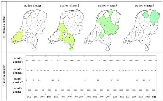
Figure 8.
Station-clusters (a) and month-clusters (b) in the BBAC_I results.
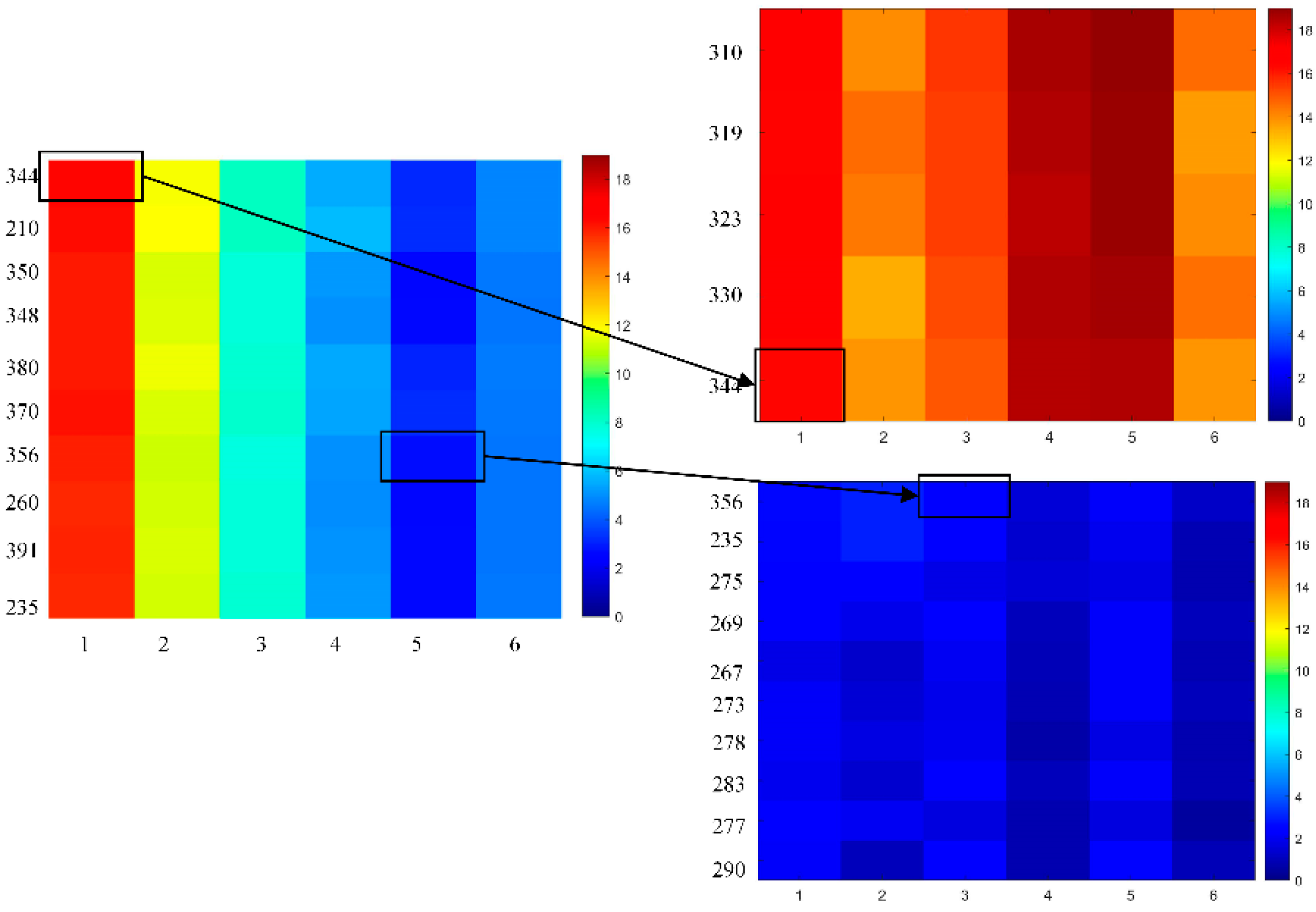
Even though the names of co-clusters with coherent trends and co-clusters with similar values reveal differences on their own, heatmaps were used to provide a more straightforward view of dissimilarities between the two. To this aim, two elements in the co-cluster2 ({Rotterdam (344), September 2000} and {Herwijnen (356), January 2001}) in the BCC_MSSR results and the corresponding co-clusters of each element in the BBAC_I results are displayed in Figure 9 as examples. As shown on the left of Figure 9, the two elements have quite different temperature values, and they were partitioned into the same co-cluster in BCC_MSSR results because of similar variations exhibited by the co-cluster, i.e., rapid deceasing and then increasing a bit. However, in the BBAC_I results where the co-clusters were divided by similar values, the two elements were partitioned into different co-clusters. The element {Rotterdam (344), September 2000} belonged to a co-cluster with all high temperatures as elements, while the element {Herwijnen (356), January 2001} belonged to another co-cluster with low temperatures.

Figure 9.
Co-cluster examples in the BCC_MSSR and BBAC_I results.
In terms of the explored patterns, the BBAC_I results discovered the spatio-temporal patterns throughout the whole study area and study period, i.e., the decreasing temperature trends from the southwest to northeast of the country, and from month-cluster1 to month-cluster4 (Figure 8). In comparison, the BCC_MSSR results explored regional coherent spatio-temporal patterns in part of the whole study area and certain time periods, e.g., first increasing and then decreasing temperatures patterns in the southwestern part of the country from May to October 2002 (Figure 5, Figure 6 and Figure 7).
As discussed above, BCC_MSSR and BBAC_I results are different in several aspects. However, there is no superior methods for all tasks. The selection of the appropriate co-clustering methods should depend on the research objective of the specific task at hand [8,44]. If the objective was to identify similar values of the attributes in the dataset, e.g., extremely high temperatures in summer, BBAC_I would be suggested. If the objective was to analyze the similar trends of the attribute at various regions, e.g., the temperature variations in different locations and their subsequent impacts, then BCC_MSSR would be considered as the suitable method.
4. Conclusions
In this study we presented the Bregman co-clustering algorithm with minimum sum-squared residue (BCC_MSSR) to analyze geo-referenced time series. Unlike previous co-clustering studies on spatio-temporal data that identify co-clusters with similar values, BCC_MSSR enables the identification of co-clusters with coherent trends, defined as exhibiting similar tendencies in the attribute(s). Using the residue as distance measure to quantify coherent trends, this algorithm regards the co-clustering issue as the minimization of the sum squared residue. To illustrate this study, Dutch monthly temperatures over 20 years at 28 stations were used as the case study. Station-clusters, month-clusters, and co-clusters in the results were displayed using small multiples, heatmaps, and line charts. Then, the BCC_MSSR results of co-clusters with coherent trends were compared with the BBAC_I results of co-clusters with similar values in terms of station-clusters, months-clusters, co-clusters, and explored spatio-temporal patterns.
Results show that the Netherlands was divided into four regions (station-clusters) from the southwest to northeast, and stations within each region have similar temperature variations. A total of 112 co-clusters with different temperature variations among them were identified in Dutch monthly temperature datasets. The 16 representative co-clusters were illustrated, and seven types of coherent temperature trends were summarized: (1) increasing; (2) decreasing; (3) first increasing and then decreasing; (4) first decreasing and then increasing; (5) first increasing, then decreasing, and finally increasing; (6) first decreasing, then increasing, and finally decreasing; (7) first decreasing, then increasing, decreasing, finally increasing. Comparisons with co-clusters of similar values show that the two co-clustering results were different: spatial distributions of station-clusters in BCC_MSSR were more stretched in space, and BCC_MSSR discovers coherent spatio-temporal patterns in local regions and certain time periods. However, the selection of the appropriate co-clustering methods should depend on the objective of the specific task at hand.
As it was the first time that BCC_MSSR was applied to geo-referenced time series, in the future there are the following directions to work on: (1) in this study we only used this co-clustering algorithm for a small dataset, in the next, we plan to apply BCC_MSSR to a larger spatio-temporal dataset to test its scalability; (2) besides geo-referenced time series, we plan to apply this algorithm to other types of spatio-temporal data, e.g., trajectories; (3) we plan to place the results of this research in broader applications, e.g., to study the impacts of obtained various temperature trends on crop yields in the Netherlands.
Funding
This research was funded by the National Natural Science Foundation of China, grant number 41901317.
Conflicts of Interest
The authors declare no conflict of interest.
References
- Ribeiro de Almeida, D.; de Souza Baptista, C.; Gomes de Andrade, F.; Soares, A. A survey on big data for trajectory analytics. ISPRS Int. J. Geo-Inf. 2020, 9, 88. [Google Scholar] [CrossRef] [Green Version]
- Li, Z.; Yang, C.; Liu, K.; Hu, F.; Jin, B. Automatic Scaling Hadoop in the Cloud for Efficient Process of Big Geospatial Data. ISPRS Int. J. Geo-Inf. 2016, 5, 173. [Google Scholar] [CrossRef] [Green Version]
- Li, Z.; Tang, W.; Huang, Q.; Shook, E.; Guan, Q. Introduction to Big Data Computing for Geospatial Applications. ISPRS Int. J. Geo-Inf. 2020, 9, 487. [Google Scholar] [CrossRef]
- Shekhar, S.; Jiang, Z.; Ali, R.Y.; Eftelioglu, E.; Tang, X.; Gunturi, V.M.V.; Zhou, X. Spatiotemporal Data Mining: A Computational Perspective. ISPRS Int. J. Geo-Inf. 2015, 4, 2306–2338. [Google Scholar] [CrossRef]
- Han, J.; Kamber, M.; Pei, J. Data Mining Concepts and Techniques, 3rd ed.; Morgan Kaufman MIT Press: Cambridge, MA, USA, 2012. [Google Scholar]
- Tatiana, V.L.; Felix, B.; Philipp, R.; Natalia, A.; Gennady, A.; Andreas, K. MobilityGraphs: Visual Analysis of Mass Mobility Dynamics via Spatio-Temporal Graphs and Clustering. IEEE Trans. Vis. Computer Graph. 2016, 22, 11–20. [Google Scholar]
- Lamb, D.S.; Downs, J.; Reader, S. Space-Time Hierarchical Clustering for Identifying Clusters in Spatiotemporal Point Data. ISPRS Int. J. Geo-Inf. 2020, 9, 85. [Google Scholar] [CrossRef] [Green Version]
- Wu, X.; Cheng, C.; Zurita-Milla, R.; Song, C. An overview of clustering methods for geo-referenced time series: From one-way clustering to co- and tri-clustering. Int. J. Geogr. Inf. Sci. 2020, 34, 1822–1848. [Google Scholar] [CrossRef]
- Andrienko, G.; Bremm, S.; Schreck, T.; Von Landesberger, T.; Bak, P.; Keim, D.; Andrienko, N. Space-in-Time and Time-in-Space Self-Organizing Maps for Exploring Spatiotemporal Patterns. Comput. Graph. Forum 2010, 29, 913–922. [Google Scholar] [CrossRef]
- Hagenauer, J.; Helbich, M. Hierarchical self-organizing maps for clustering spatiotemporal data. Int. J. Geogr. Inf. Sci. 2013, 27, 2026–2042. [Google Scholar] [CrossRef]
- Liu, L.; Hu, T.; Bao, S.; Wu, H.; Peng, Z.; Wang, R. The Spatiotemporal Interaction Effect of COVID-19 Transmission in the United States. ISPRS Int. J. Geo-Infation 2021, 10, 387. [Google Scholar] [CrossRef]
- Ahas, R.; Aasa, A.; Silm, S.; Roosaare, J. Seasonal Indicators and Seasons of Estonian Landscapes. Landsc. Res. 2005, 30, 173–191. [Google Scholar] [CrossRef]
- Wu, X.; Zurita-Milla, R.; Kraak, M.-J. Visual discovery of synchronization in weather data at multiple temporal resolutions. Cartograph. J. 2013, 50, 247–256. [Google Scholar] [CrossRef]
- Wu, X.; Zurita-Milla, R.; Kraak, M.-J. Co-clustering geo-referenced time series: Exploring spatio-temporal patterns in Dutch temperature data. Int. J. Geogr. Inf. Sci. 2015, 29, 624–642. [Google Scholar] [CrossRef] [Green Version]
- Wu, X.; Zurita-Milla, R.; Kraak, M.-J. A novel analysis of spring phenological patterns over Europe based on co-clustering. J. Geophys. Res. Biogeosci. 2016, 121, 1434–1448. [Google Scholar] [CrossRef] [Green Version]
- Wu, X.; Cheng, C.; Qiao, C.; Song, C. Spatio-temporal differentiation of spring phenology in China driven by temperatures and photoperiod from 1979 to 2018. Sci. China Earth Sci. 2020, 63, 1485–1498. [Google Scholar] [CrossRef]
- Ullah, S.; Daud, H.; Dass, S.C.; Khan, H.N.; Khalil, A. Detecting space-time disease clusters with arbitrary shapes and sizes using a co-clustering approach. Geospat. Heal. 2017, 12. [Google Scholar] [CrossRef] [Green Version]
- Andreo, V.; Izquierdo-Verdiguier, E.; Zurita-Milla, R.; Rosà, R.; Rizzoli, A.; Papa, A. Identifying Favorable Spatio-Temporal Conditions for West Nile Virus Outbreaks by Co-Clustering of Modis LST Indices Time Series. In Proceedings of the IGARSS 2018—2018 IEEE International Geoscience and Remote Sensing Symposium, Valencia, Spain, 22–27 July 2018; pp. 4670–4673. [Google Scholar]
- Liu, Q.; Zheng, X.; Stanley, H.E.; Xiao, F.; Liu, W. A Spatio-Temporal Co-Clustering Framework for Discovering Mobility Patterns: A Study of Manhattan Taxi Data. IEEE Access 2021, 9, 34338–34351. [Google Scholar] [CrossRef]
- Eisen, M.B.; Spellman, P.T.; Brown, P.O.; Botstein, D. Cluster analysis and display of genome-wide expression patterns. Proc. Natl. Acad. Sci. USA 1998, 95, 14863–14868. [Google Scholar] [CrossRef] [Green Version]
- Kriegel, H.-P.; Kröger, P.; Zimek, A. Clustering high-dimensional data: A survey on subspace clustering, pattern-based clustering, and correlation clustering. ACM Trans. Knowl. Discov. Data 2009, 3, 1. [Google Scholar] [CrossRef]
- Liang, L.; Li, L.; Liu, Q. Precipitation variability in Northeast China from 1961 to 2008. J. Hydrol. 2011, 404, 67–76. [Google Scholar] [CrossRef]
- Alexander, L.V.; Uotila, P.; Nicholls, N. Influence of sea surface temperature variability on global temperature and precipi-tation extremes. J. Geophys. Res. Atmos. 2009, 114, 1–13. [Google Scholar]
- Estay, S.A.; Clavijo-Baquet, S.; Lima, M.; Bozinovic, F. Beyond average: An experimental test of temperature variability on the population dynamics of Tribolium confusum. Popul. Ecol. 2010, 53, 53–58. [Google Scholar] [CrossRef]
- Zanobetti, A.; O’Neill, M.S.; Gronlund, C.J.; Schwartz, J.D. Summer temperature variability and long-term survival among elderly people with chronic disease. Proc. Natl. Acad. Sci. USA 2012, 109, 6608–6613. [Google Scholar] [CrossRef] [PubMed] [Green Version]
- Andresen, M.A.; Malleson, N. Crime seasonality and its variations across space. Appl. Geogr. 2013, 43, 25–35. [Google Scholar] [CrossRef]
- Banerjee, A.; Dhillon, I.; Ghosh, J.; Merugu, S.; Modha, D.S. A generalized maximum entropy approach to bregman co-clustering and matrix approximation. J. Mach. Learn. Res. 2007, 8, 1919–1986. [Google Scholar]
- Cheng, Y.; Church, G.M. Biclustering of expression data. In Proceedings of the Proceedings ISMB 2000, San Diego, CA, USA, 19–23 August 2000; pp. 93–103. [Google Scholar]
- Cho, H.; Dhillon, I.S.; Guan, Y.; Sra, S. Minimum Sum-Squared Residue Co-clustering of Gene Expression Data. In Proceedings of the 2004 SIAM International Conference on Data Mining; Society for Industrial & Applied Mathematics (SIAM), Philadelphia, PA, USA, 22–24 April 2004. [Google Scholar]
- Cho, H.; Dhillon, I. Coclustering of Human Cancer Microarrays Using Minimum Sum-Squared Residue Coclustering. IEEE/ACM Trans. Comput. Biol. Bioinform. 2008, 5, 385–400. [Google Scholar] [CrossRef]
- Yang, J.; Wang, H.; Wang, W.; Yu, P. Enhanced biclustering on expression data. In Proceedings of the Third IEEE Symposium on Bioinformatics and Bioengineering, Bethesda, MD, USA, 12 March 2003; pp. 321–327. [Google Scholar]
- Kluger, Y.; Basri, R.; Chang, J.T.; Gerstein, M. Spectral Biclustering of Microarray Data: Coclustering Genes and Conditions. Genome Res. 2003, 13, 703–716. [Google Scholar] [CrossRef] [Green Version]
- Rathipriya, R.; Thangavel, K.; Bagyamani, J. Binary Particle Swarm Optimization based Biclustering of Web Usage Data. Int. J. Comput. Appl. 2011, 25, 43–49. [Google Scholar] [CrossRef]
- Rousseeuw, P.J. Silhouettes: A graphical aid to the interpretation and validation of cluster analysis. J. Comput. Appl. Math. 1987, 20, 53–65. [Google Scholar] [CrossRef] [Green Version]
- Lewis, J.M.; Ackerman, M.; Sa, V.R.D. Human cluster evaluation and formal quality measures: A comparative study. In Proceedings of the 34th Conference of the Cognitive Science Society (CogSci), Sapporo, Japan, 1–4 August 2012; Volume 34, pp. 1870–1875. [Google Scholar]
- Wu, X.; Zurita-Milla, R.; Verdiguier, E.I.; Kraak, M.-J. Triclustering Georeferenced Time Series for Analyzing Patterns of Intra-Annual Variability in Temperature. Ann. Am. Assoc. Geogr. 2017, 108, 71–87. [Google Scholar] [CrossRef] [Green Version]
- Visser, H. The Significance of Climate Change in the Netherlands. An Analysis of Historical and Future Trends (1901–2020) in Weather Conditions, Weather Extremes and Temperature-Related Impacts. MNP Rep. 2005, 550002007. Available online: https://www.pbl.nl/en/publications/The_significance_of_climate_change_in_the_Netherlands (accessed on 5 January 2022).
- Garssen, J.; Harmsen, C.; De Beer, J. The effect of the summer 2003 heat wave on mortality in the Netherlands. Eurosurveillance 2005, 10, 13–14. [Google Scholar] [CrossRef]
- Fischer, P.H.; Marra, M.; Ameling, C.B.; Janssen, N.; Cassee, F.R. Trends in relative risk estimates for the association between air pollution and mortality in The Netherlands, 1992–2006. Environ. Res. 2011, 111, 94–100. [Google Scholar] [CrossRef] [PubMed]
- Daniels, E.E.; Lenderink, G.; Hutjes, R.W.A.; Holtslag, A.A.M. Spatial precipitation patterns and trends in The Netherlands during 1951–2009. Int. J. Clim. 2014, 34, 1773–1784. [Google Scholar] [CrossRef]
- van Vliet, A.J.H.; Overeem, A.; De Groot, R.S.; Jacobs, A.F.G.; Spieksma, F.T.M. The influence of temperature and climate change on the timing of pollen release in the Netherlands. Int. J. Clim. 2002, 22, 1757–1767. [Google Scholar] [CrossRef]
- Schaap, B.F.; Blom-Zandstra, M.; Hermans, C.M.L.; Meerburg, B.; Verhagen, J. Impact changes of climatic extremes on arable farming in the north of the Netherlands. Reg. Environ. Chang. 2011, 11, 731–741. [Google Scholar] [CrossRef] [Green Version]
- Shao, J.; Li, Y.; Ni, J. The characteristics of temperature variability with terrain, latitude and longitude in Sichuan-Chongqing Region. J. Geogr. Sci. 2012, 22, 223–244. [Google Scholar] [CrossRef]
- Grubesic, T.H.; Wei, R.; Murray, A.T. Spatial Clustering Overview and Comparison: Accuracy, Sensitivity, and Computational Expense. Ann. Assoc. Am. Geogr. 2014, 104, 1134–1156. [Google Scholar] [CrossRef]


Publisher’s Note: MDPI stays neutral with regard to jurisdictional claims in published maps and institutional affiliations. |
© 2022 by the author. Licensee MDPI, Basel, Switzerland. This article is an open access article distributed under the terms and conditions of the Creative Commons Attribution (CC BY) license (https://creativecommons.org/licenses/by/4.0/).