3D Modeling of Individual Trees from LiDAR and Photogrammetric Point Clouds by Explicit Parametric Representations for Green Open Space (GOS) Management

Abstract

The development and management of green open spaces are essential in overcoming environmental problems such as air pollution and urban warming. 3D modeling and biomass calculation are the example efforts in managing green open spaces. In this study, 3D modeling was carried out on point clouds data acquired by the UAV photogrammetry and UAV LiDAR methods. 3D modeling is done explicitly using the point clouds fitting method. This study uses three fitting methods: the spherical fitting method, the ellipsoid fitting method, and the spherical harmonics fitting method. The spherical harmonics fitting method provides the best results and produces an R² value between 0.324 to 0.945. In this study, Above-Ground Biomass (AGB) calculations were also carried out from the modeling results using three methods with UAV LiDAR and Photogrammetry data. AGB calculation using UAV LiDAR data gives better results than using photogrammetric data. AGB calculation using UAV LiDAR data gives an accuracy of 78% of the field validation results. However, for visualization purposes with a not-too-wide area, a 3D model of photogrammetric data using the spherical harmonics method can be used.

1. Introduction

Global environmental change is an ongoing issue and has been widely discussed from various perspectives. Three main factors contributing to global environmental change are increased concentrations of carbon dioxide in the atmosphere, changes in the global adhesion cycle, and changes in land cover and land use [1]. The increase in carbon dioxide concentration mainly occurs in urban areas, which account for more than 70% of carbon dioxide emissions [2]. Rapid population growth is the main factor contributing to the increase in carbon dioxide concentrations [3]. A 1% increase in population is associated with a 1.28% increase in carbon dioxide emissions [4]. Rapid population growth has resulted in many changes in land use from green open spaces to more economical land uses such as settlements and offices. Land use change is also related to the third factor of changes in the global environment. At the same time, the ecological balance of the urban environment is as important as the development of the economic value of urban areas. Excessive development in urban areas results in reduced green open space and causes environmental problems such as urban warming and air pollution. Urban warming and increasing air pollution in cities cause many harmful effects, such as health problems [5].

Urban green open spaces have essential ecological benefits [6]. Green open space in the global development environment is currently needed to maintain the balance of the environmental quality of an area, especially in urban areas that have various problems related to such complex spatial problems. Based on the rules contained in Article 29 paragraph 2 of Law number 26 of 2007 concerning Spatial Planning applicable in Indonesia, it is stated that the proportion of green open space in an urban area should be at least 30 percent of the city’s total area. Preservation and development of green open spaces are two of the strategic efforts in reducing urban environmental pollution because trees can naturally absorb CO gas which is stored in the form of carbon compounds and released in the form of oxygen while absorbing heat so that it lowers the ambient air temperature [7].

Some solutions to urban warming and increasing air pollution in urban areas are replanting critical lands and managing existing green open spaces by mapping and building tree databases. Currently, the mapping of green open spaces and the construction of tree databases are still based on a Geographic Information System (GIS) based on two-dimensional (2D) data. At the same time, a three-dimensional (3D) model has a visual representation that is closer to the actual shape so that it will produce a better product. Based on this, a 3D model for tree database creation is needed to manage green open space. In the 3D modeling of an object, the term Level of Detail (LOD) is known. LOD is used to describe the level of detail from the geometric and semantic aspects of the 3D model. The higher the LOD used, the more detailed the 3D model. The difference in LOD will affect the results of the analysis carried out. For example, [8] performs 3D object analysis of individual trees to estimate the intensity of shadows around trees. Individual trees with higher LOD give better results or are closer to the actual situation. The research shows that individual tree modeling at high LOD levels for large areas is needed to perform a better urban area analysis. The 3D model of a tree can be used as the basis of the database, and a more comprehensive spatial analysis can be carried out.

As the input data for 3D tree modeling, the acquisition of point clouds data has been widely carried out using Unmanned Aerial Vehicles (UAV). UAVs can already carry cameras and LiDAR sensors of various types and sizes. UAVs carrying cameras and LiDAR sensors have been widely used to carry out forestry management in Indonesia for both government and private agencies. This is because the UAV is relatively cheaper than conventional methods and covers a broader area in a shorter time. In addition, the accuracy of the products produced by UAV LiDAR and UAV photogrammetry data is growing over time, which makes the use of these vehicles and sensors also increase.

3D modeling of individual tree objects can be done implicitly or explicitly. Explicit individual tree modeling can be done by performing surface fittings on point clouds data from field acquisition. The fitting methods used are quite diverse, from the simplest method utilizing a sphere shape to a complicated method utilizing a spherical harmonics approach. Explicit 3D modeling with this fitting method is done automatically to speed up the process and reduce the human resources involved. This paper aims to perform individual 3D tree modeling explicitly and automatically using the UAV LiDAR and UAV photogrammetry data.

The paper is divided as follows: Section 1 explains the urgency of building a 3D model in managing green open space using LiDAR and photogrammetry point clouds data. Section 2 will discuss some related works in 3D modeling of the individual tree, the use of CityGML, and the method of determining the biomass. Section 3 will describe the proposed workflow and explain the methods used in the data processing section. Section 4 will present the results of research that has been carried out, such as the selection of the Diameter Breast Height (DBH), the creation of a canopy and trunk model using three surface fitting methods, the creation of a 3D model in CityGML format, and the calculation of biomass in the area of interest. Section 5 is a discussion and analysis of the results that have been presented in Section 4. Section 6 is the conclusion of the research that has been done.

2. Related Work

At this time, the need for 3D data is increasing, considering that 3D data can be used for various purposes, one of which is to analyze urban areas. 3D models in an urban area will include buildings, roads, vegetation, water bodies, and soil, which can be used in various applications [9]. 3D models can be divided into two applications: applications based on visualization and those not based on visualization [10]. Examples of applications using a 3D model are noise propagation analysis in an area [11,12], 3D cadaster [13], facility management [14], solar radiation estimation analysis [15], energy demand estimation in an area [16], and urban water demand [17].

Rapid technological developments impact the development of increasingly sophisticated data acquisition techniques. A 3D model can be obtained from various acquisition techniques [9], for example photogrammetry [18], laser scanning [19,20,21], extrusion from 2D sites [22], Synthetic Aperture Radar (SAR) [23,24], and architectural drawings and models.

The objects of the 3D model of the urban area are stored in a City Geography Markup Language (CityGML) data model. CityGML is an XML-based data model used to describe the geometry and attributes of 3D objects [25]. In addition, CityGML describes the relationship and hierarchical structure of a 3D object in five levels of LOD. LOD is a term used to define the level of detail of a 3D model and has implications for specific applications [26,27]. In [8], it is explained about the redefinition of the individual tree LOD into 14 classes, namely from LOD 0.A to LOD 3.D.

Individual tree modeling can be done using various methods. One method that has been carried out at this time is by segmenting each tree object to obtain information about the tree’s position, height, and diameter of the canopy [28]. Modeling is done implicitly based on tree parameter data. For a broader application, the paper [29] describes the modeling of individual trees in the Singapore Botanical Gardens Area on LOD1 and LOD2 simultaneously from UAV LiDAR point clouds data. Explicit modeling of the individual tree can be carried out using the spherical fitting, ellipsoidal fitting, and spherical harmonics fitting methods. Spherical harmonics is a particular function used to define the surface of a sphere. The spherical harmonics method can accurately model objects [30]. Spherical harmonics is often used in solving partial differential equations in many scientific fields. 3D modeling using the spherical harmonics method has been carried out in research [30] to model cells accurately.

One of the methods for managing green open spaces is biomass calculation. There are four main ways to calculate biomass: in situ destructive samplings, non-destructive sampling with in situ forest data collection, estimation through remote sensing, and model making This method uses the fourth method, which calculates biomass by making a model. The results of 3D modeling generated from data acquisition can calculate biomass. Modeling can be done using various survey methods. Survey methods that are often used to calculate biomass are scanning using Terrestrial Laser Scanner (TLS) [31,32], UAV LiDAR method [33,34], and UAV photogrammetry method [35,36]. Parameters obtained from the survey results are DBH, tree height, and canopy width. These parameters are the primary basis for calculating biomass using allometric equations. One of the commonly used allometric equations is the equation of [37]. In addition to determining the value of DBH on trees, volume calculation is also one of the methods for managing individual trees in green open space. In [38], 3D modeling of individual trees was carried out directly on point clouds data using surface reconstruction concave hull and 3D alpha shape methods to calculate the tree canopy volume. The data used in this study were acquired using a LiDAR UAV. Meanwhile, in the study [39], the calculation of the canopy volume was carried out on the data acquired by the TLS using the concave hull method.

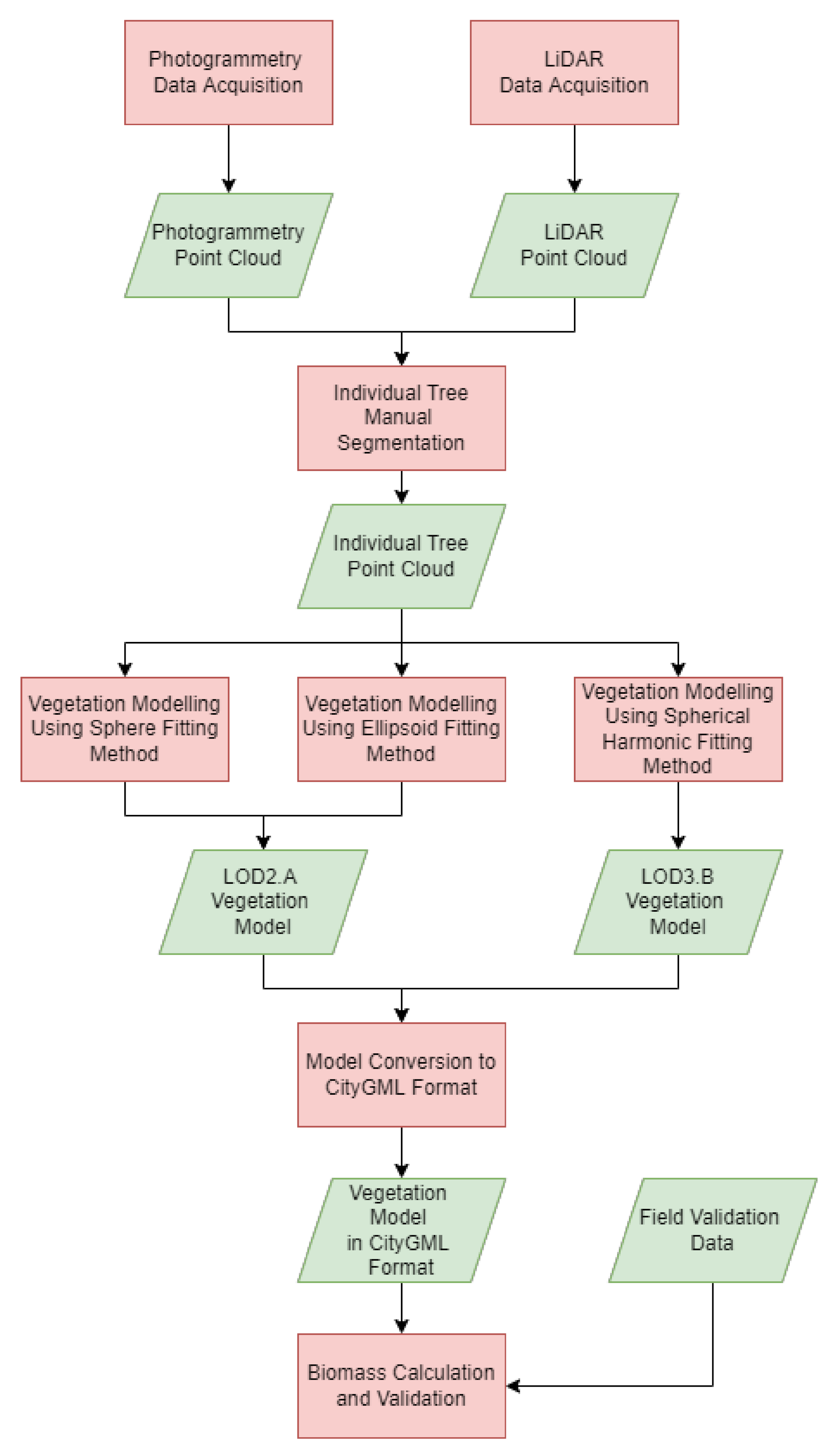
3. Data and Employed Methods

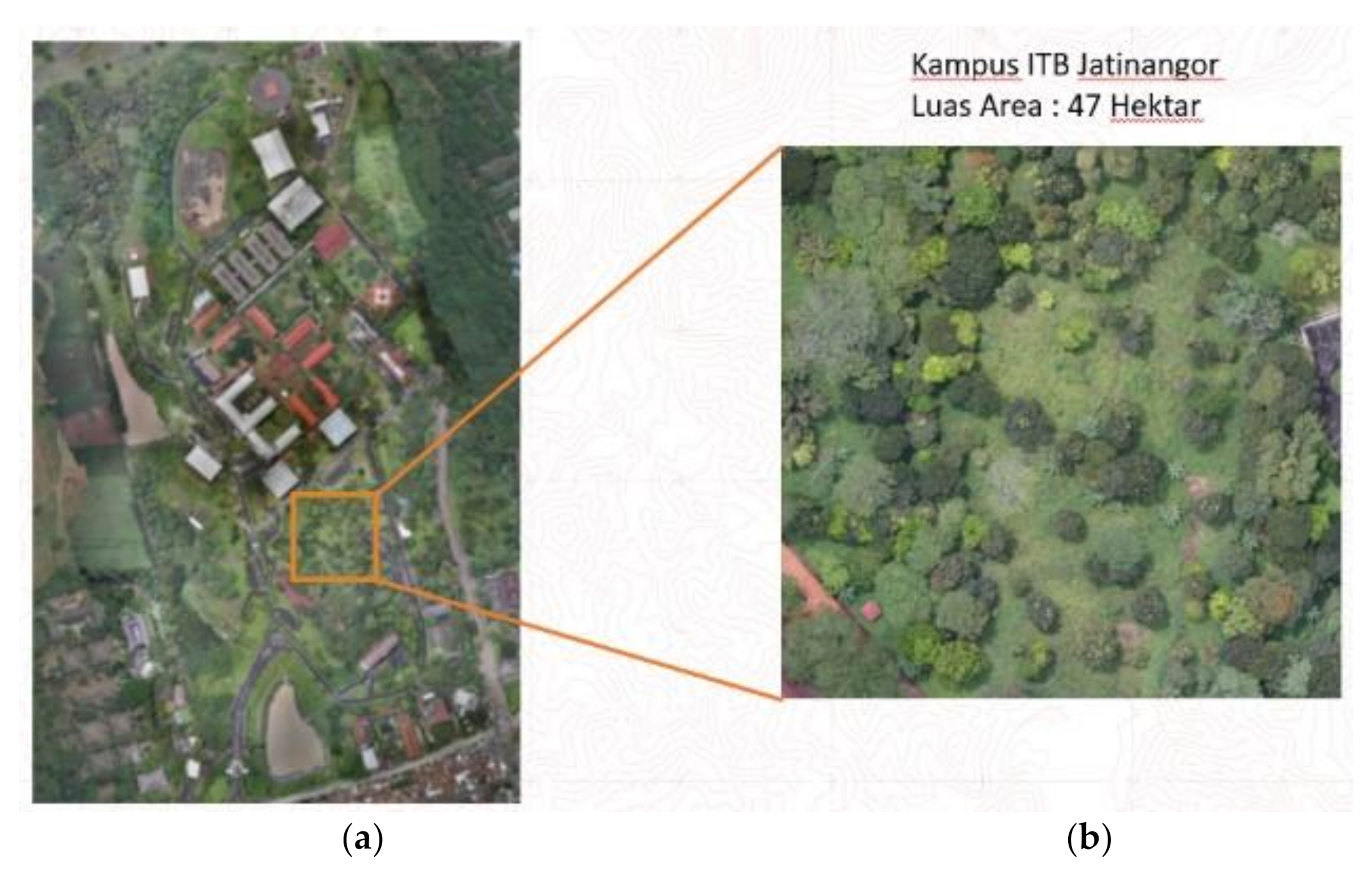
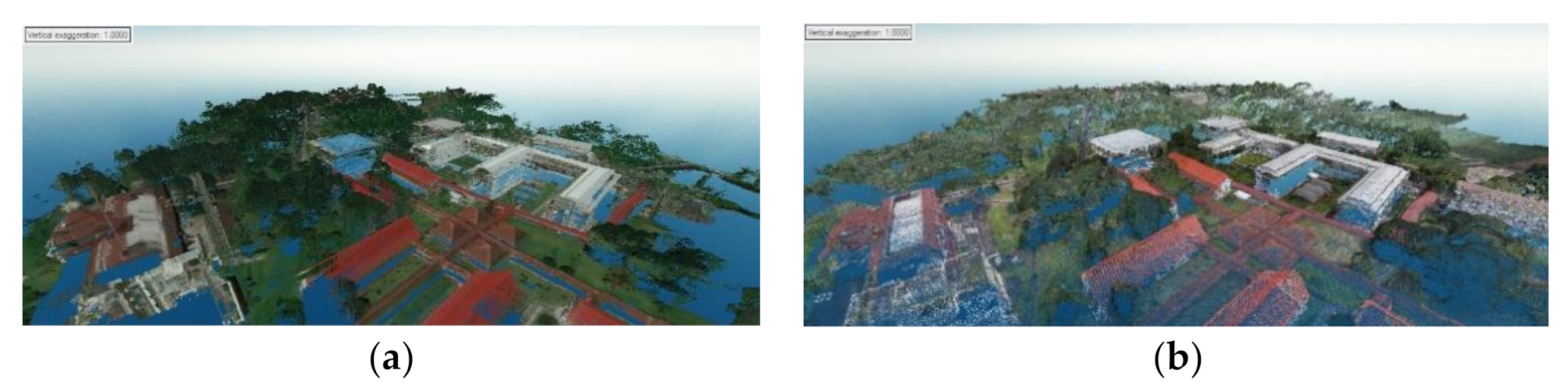
3.1. Data

The research was conducted at the Bandung Institute of Technology (ITB) Jatinangor Campus (6°55′40.6″ S 107°46′08.9″ E, 776 m above sea level), which has an area of 47 ha. The ITB Jatinangor Campus was chosen because it has diverse vegetation categorized as green open spaces. 3D modeling was performed on one of the small sections marked in Figure 1, which has an area of 1 ha.

LiDAR data was acquired using a Hesai Pandar 40 LiDAR sensor mounted on a DJI Matrice 600. The UAV flies at an altitude of 50 m at 1 m/s. The data acquisition was carried out in three UAV flight processes, resulting in three data point clouds with their respective UAV flight paths. The LiDAR point clouds product was tested using 18 Independent Check Points (ICPs) measured using the GNSS rapid static method and had a Z coordinate accuracy of 0.248 m and a density of 120 points per m².

Photogrammetric data was acquired using a Sony Alpha 6000 camera mounted on a UAV VTOL. The UAV flies at an altitude of 150 m with a sidelap and overlap value of 80%. The UAV used has a Post Processing Kinematic (PPK) aerial control point system so that each photo has precise coordinates of the exposure point. The photogrammetric process is processed using the Agisoft Metashape software with the Structure form Motion (SfM) method to generate point clouds.

The quality of the photogrammetric products was tested using 19 ICPs. The ICPs were measured using the rapid static method for 20 min. The results of the accuracy test of the photogrammetric product can be seen in

Table 1. RMSE checkpoint for photogrammetric products.

Number of Points	RMSE
	X (cm)	Y (cm)	Z (cm)
19	4.62	3.35	10.67

. Photogrammetric point clouds have a density of 10 points per m².

The point clouds data generated by UAV LiDAR and UAV photogrammetry methods can be seen in Figure 2.

The characteristics of the point clouds generated by the LiDAR acquisition method and photogrammetry can be seen from the cross-section, as shown in Figure 3. UAV photogrammetry point clouds look more complete than UAV LiDAR point clouds data, as seen in the tree and building objects in Figure 3. This is because photogrammetry processing uses the dense image matching principle, which performs interpolation, in contrast to LiDAR point clouds, which are obtained directly from the laser reflection hitting the object. The different characteristics between UAV photogrammetry point clouds and UAV LiDAR point clouds will affect the results of individual tree 3D modeling, both in terms of shape and size.

In the UAV LiDAR point clouds data, the shape of the individual tree can be seen clearly, in contrast to the photogrammetric point clouds, which is only the surface of the canopy, as seen in Figure 4. The point clouds data are then segmented manually by digitizing the existing orthophotos data. The point clouds data from LiDAR and photogrammetry are then cut based on the vector data that has been created previously. Prior to modeling, the canopy portion of the tree was selected manually. Manual digitation is done so that the results of the canopy modeling carried out in the next stage have high accuracy.

3.2. Method

The flow chart of the research methodology can be seen in Figure 5. The stage begins with acquiring field data using two methods: UAV photogrammetry and UAV LiDAR. The UAV LiDAR method produces detailed point clouds because of its ability to perform multiple reflections on the laser used. In addition, LiDAR data has also been proven effective in forestry management purposes. Meanwhile, UAV photogrammetry is a low-cost data acquisition method widely used for topographic mapping and 3D modeling. Next, the point clouds are segmented manually. Segmentation is done to separate individual tree objects from other objects. The segmented individual tree point clouds are processed to obtain a solid individual tree 3D model. Calculations of tree geometry, such as tree trunks and crowns, are more effective in solid shapes. In addition, the 3D model that has been created is entered into a 3D database of green open space, which consists of geometric data of 3D models and semantic data from individual trees. The results of 3D modeling of the individual tree obtained from the two methods are compared, considering their respective advantages and disadvantages. In the end, the biomass calculation is done for both UAV LiDAR data and UAV photogrammetry data.

3.2.1. Best Fitting Method

Three data fitting methods are used to perform 3D modeling of the individual tree: the spherical fitting method, the ellipsoid fitting method, and the spherical harmonics fitting method. The spherical fitting method uses the least squares principle to find the optimal value of the center point of the point clouds and the sphere’s radius [40]. The mathematical equation of the circle is, as can be seen in Equation (1).

$${\left(x_i-x\right)}^2+{\left(y_i-y\right)}^2+{\left(z_i-z\right)}^2=r^2$$

(1)

Equation (1) is then written in the form of a function as shown in Equation (2) and extended into a function in Equation (3).

$$\mathrm{F}={{\displaystyle \sum }}_{i=1}^{n}f{i}^2={{\displaystyle \sum }}_{i=1}^n{\left({\left(x_i-x\right)}^2+{\left(y_i-y\right)}^2+{\left(z_i-z\right)}^2-r^2\right)}^2$$

(2)

$$f_i=-2x_{i}x-2y_{i}y-2z_{i}z+\left(x_i{}^2+y_i{}^2+z_i{}^2\right)+\left(x_i{}^2+y_i{}^2+z_i{}^2-r^2\right)$$

(3)

$\left(x_i{}^2+y_i{}^2+z_i{}^2-r^2\right)$ can be symbolized as α, so Equation (3) has four parameters: x, y, z, and α. The equation can be solved by using matrix operations, as shown in Equation (4).

$$X={\left[A^{T}A\right]}^{-1}\left[A^{T}B\right]$$

(4)

The value of the sphere radius can be calculated by Equation (5).

$$r=\sqrt{x_i{}^2+y_i{}^2+z_i{}^2-\mathsf{\alpha }}$$

(5)

Not much different from spherical fitting, the ellipsoid fitting method uses the least square principle to find the optimal value of the center point of the point clouds and the flattening parameter of the ellipsoid. The general equation of the ellipsoid is shown in Equation (6).

$$A^{\prime }{x}^2+B^{\prime }{y}^2+C^{\prime }{z}^2+2D^{\prime }xy+2E^{\prime }xz+2F^{\prime }yz+2G^{\prime }x+2H^{\prime }y+2I^{\prime }z+K^{\prime }=0$$

(6)

Equation (6) has ten parameters, but these nine parameters are independent. Equation (6) can be converted into Equation (7) so that it only has nine parameters. Equation (7) is a linear equation that can be solved by the least square method.

$$A{x}^2+B{y}^2+C{z}^2+2Dxy+2Exz+2Fyz+2Gx+2Hy+2Iz-1=0$$

(7)

The third method used is the spherical harmonics fitting method. Spherical harmonics is a natural selection of the Basis functions representing all double differential spherical functions. Spherical harmonics can be defined as complex functions of order l and degree m, seen in Equation (8).

$$Y_l^m\left(\mathsf{\theta },\mathsf{\phi }\right)=\sqrt{\frac{2l+1}{4\pi } \frac{\left(lm\right)!}{\left(l+m\right)!}{p}_l^m\left(cos\mathsf{\theta }\right)\exp im\mathsf{\phi }}$$

(8)

where l and m are integers such that |m| ≤ l, and $p_l^m$ are associated Legendre polynomials [30]. Any spherical function f (θ, φ) can be represented by a linear combination of spherical harmonics $Y_l^m$ (θ, φ) as shown in Equation (9).

$$f\left(\mathsf{\theta },\mathsf{\phi }\right)={\displaystyle \sum }_{l=0}^{\infty }{\displaystyle \sum }_{m=-1}^l{a}_l^m{Y}_l^m\left(\mathsf{\theta },\mathsf{\phi }\right)$$

(9)

Equation (9) is then converted into a matrix form, and the variables contained in the equation are solved using the least square method.

3.2.2. Accuracy Assesment of Best Fitting

The segmented point clouds are then 3D modeled. The resulting 3D model is saved in surface format stored in the faces and vertices table. The goodness of fit (R²) value is then calculated to see the quality of the modeling results. The value of R² is calculated using a formula in Equation (10).

$$R^2=1-\frac{RSS}{TSS}$$

(10)

where RSS is the sum of the square of residuals obtained from subtracting the distance from the point to the center point of the point clouds with the distance to the modeling surface. TSS is an abbreviation of total sum square, which is sum of the squares of the distance value from the center point minus the average data distance from the center point. In other words, TSS is the value of the distance variance. The calculation of the R² value is carried out on the modeling results using UAV photogrammetry and UAV LiDAR data.

3.2.3. Diameter Breast Height and Biomass Calculation

Diameter Breast Height (DBH) can be modeled by finding the equation of the relationship with the radius of the tree crown canopy. Some of the equations of the mathematical model built in this study are expressed in Equation (11) to Equation (14).

$$\mathrm{Linear}: D=b_0+b_{1}r$$

(11)

$$\mathrm{Power}: D=b_0 r^{b1}$$

(12)

$$\mathrm{Polynomial}: D=b_0 r^2+b_1 r+b_2$$

(13)

$$\mathrm{Logarithmic}: D=b_0 \ln \left(r\right)$$

(14)

where D is the estimated DBH value, r is the value of the measured tree crown radius, and b is the coefficient of the equation.

Biomass is the total weight or volume of organisms in a particular area or volume. Biomass is also defined as the total amount of living matter above the surface of a tree and is expressed in metric tons of dry weight per unit area [41]. Forest biomass plays an essential role in the biogeochemical cycle, especially in the carbon cycle. Of the total forest carbon, about 50% of it is stored in forest vegetation [42]. The dynamics of carbon in nature can be explained simply by the carbon cycle. The carbon cycle is a biogeochemical cycle that includes carbon exchange between the biosphere, pedosphere, geosphere, hydrosphere, and Earth’s atmosphere. The carbon cycle is complex, and each process affects the other processes.

The biomass allometric model is a statistical model for estimating tree biomass based on tree diameter or height [43] and wood density as an important variable in estimating biomass in tropical forests [37]. Therefore, to support the accurate estimation of biomass and carbon stocks, it is necessary to develop biomass allometric models for various tree species and growing locations [44].

4. Results

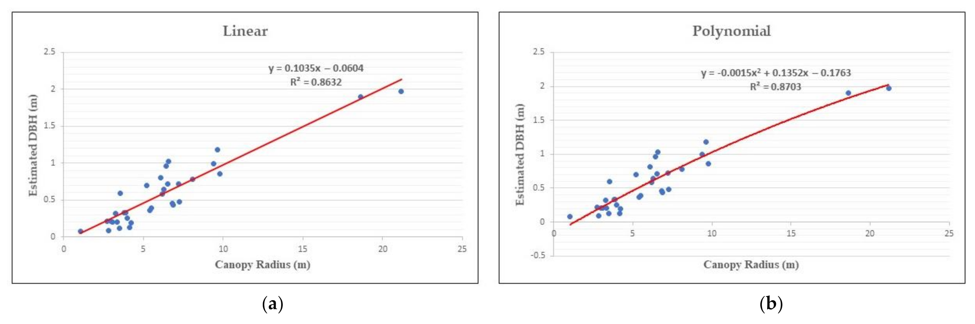
4.1. Diameter Breast Height (DBH) Model

Accurate modeling of forest structural parameters is essential for forest operational management, forest inventories, and carbon cycle modeling [45]. The tree trunk is one of the most fundamental components of the forest structure and needs to be modelled accurately. The tree trunk model is based on the DBH parameters. The DBH value is not only used as a parameter for 3D modeling. It can also estimate AGB to calculate carbon stocks in a forest.

The estimated value of DBH can be calculated from the regression model of the relationship with other tree parameters such as tree crown radius and tree height. In this research, the DBH of the tree is estimated from the value of the tree crown radius that can be known from the point clouds acquired by UAV LiDAR and UAV photogrammetry methods. DBH values were measured directly in the field for 33 tree points to make the DBH model. The value of the radius of the canopy was obtained by calculating the radius of the point clouds from the canopy using the least squares method. The relationship between the DBH due to the field measurements and the radius of the estimated crown is sought using several equations, namely linear, power, polynomial, and logarithmic. A correlation test of the tree crown radius with the DBH variable from field measurements was carried out to select DBH estimation variables. The most robust correlation value is used as a variable in the estimation of tree DBH. The scatter plot of the relationship between the DBH of the tree and the radius of the tree crown can be seen in Figure 6.

The regression graph of each method can be seen in Figure 7, and the coefficient values for each equation can be seen in

Table 2. The equation and R² of each regression method for estimating Diameter Breast Height.

Regression Model	Equation	R2
Linear	D = 0.1035r − 0.0604	0.863
Polynomial	D = −0.0015r2 + 0.1352r − 0.1763	0.870
Power	D = 0.0546r1.2476	0.847
Logarithmic	D = 0.6824ln(r) − 0.5473	0.752

, where r is the tree crown radius and D is the DBH. The regression graphs generated by linear, power, and polynomial equations do not differ much. This is caused by the relationship between the tree crown radius and DBH, which tends to be linear. The coefficient of the power equation is close to a value of 1, which is 1.2476, and the quadratic coefficient of the polynomial equation is very small, which is −0.0015. In contrast, the logarithmic equation produces a different graph from the other equations. Regression using logarithmic equations tends to ignore data with large tree crown radius and DBH values due to the small amount of data in the cluster.

The regression results produce equations and the R² value from each equation used. Table 2 shows that the polynomial equation has the largest R² value among other equations. The equation and R² value of each regression method can be seen in Table 2. The polynomial method’s regression results are then used to calculate the DBH value, which will be used to create a 3D model of the tree and calculate AGB because it has the largest R² value among other equations.

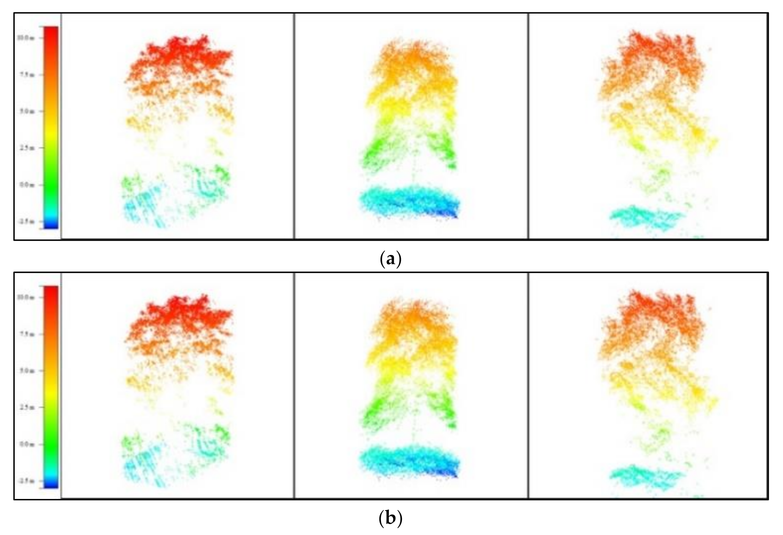
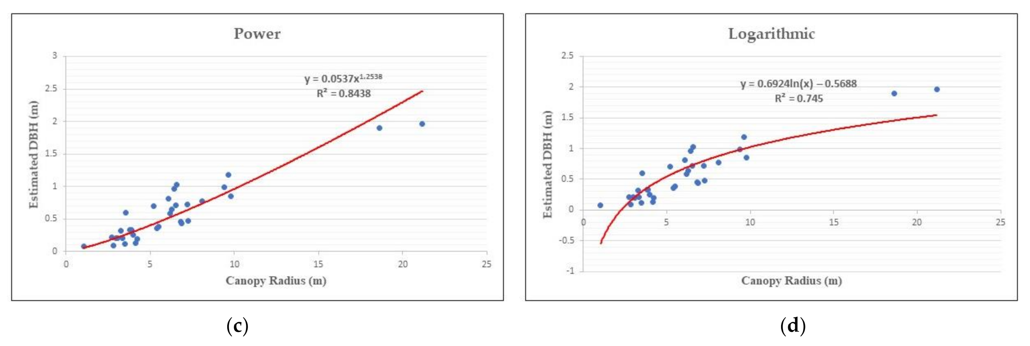
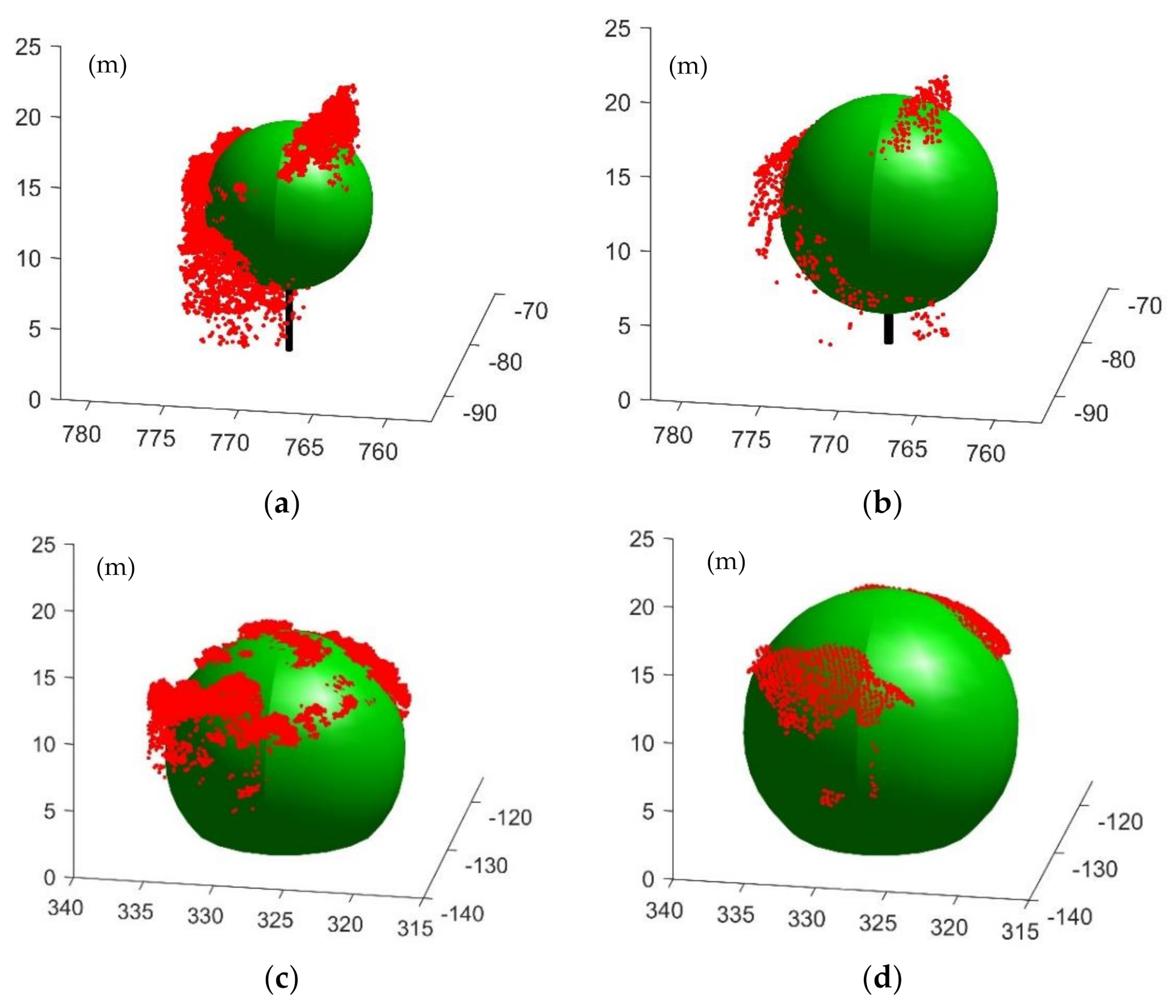
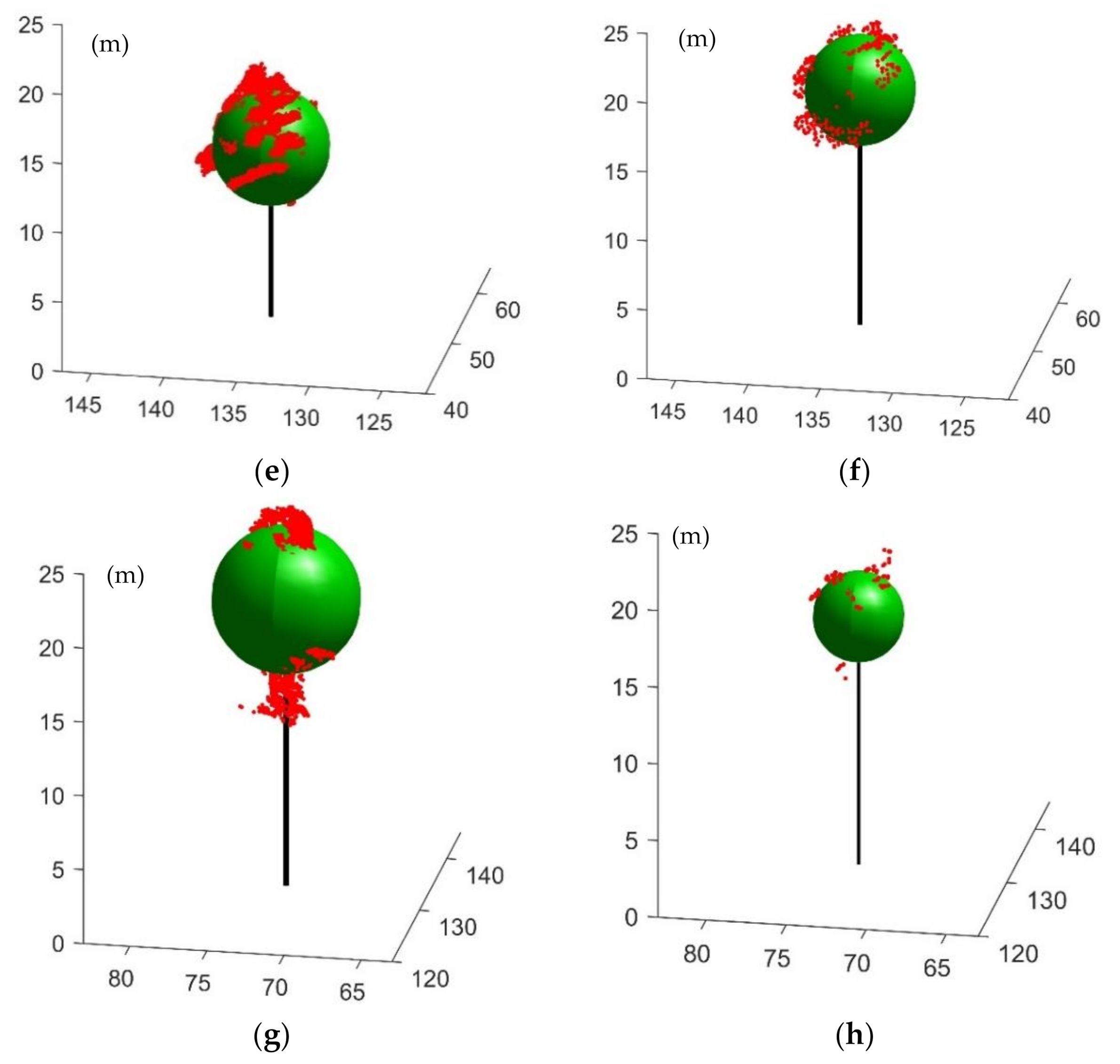
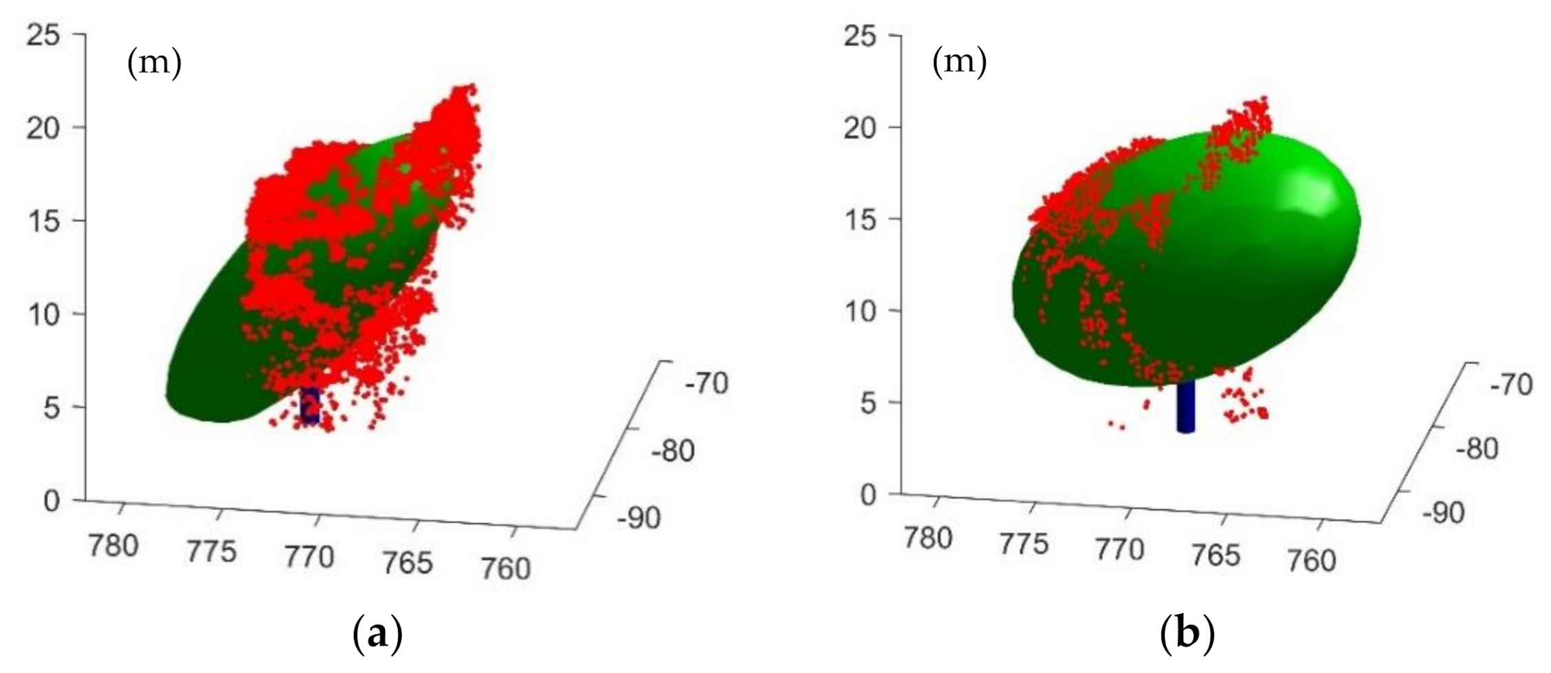
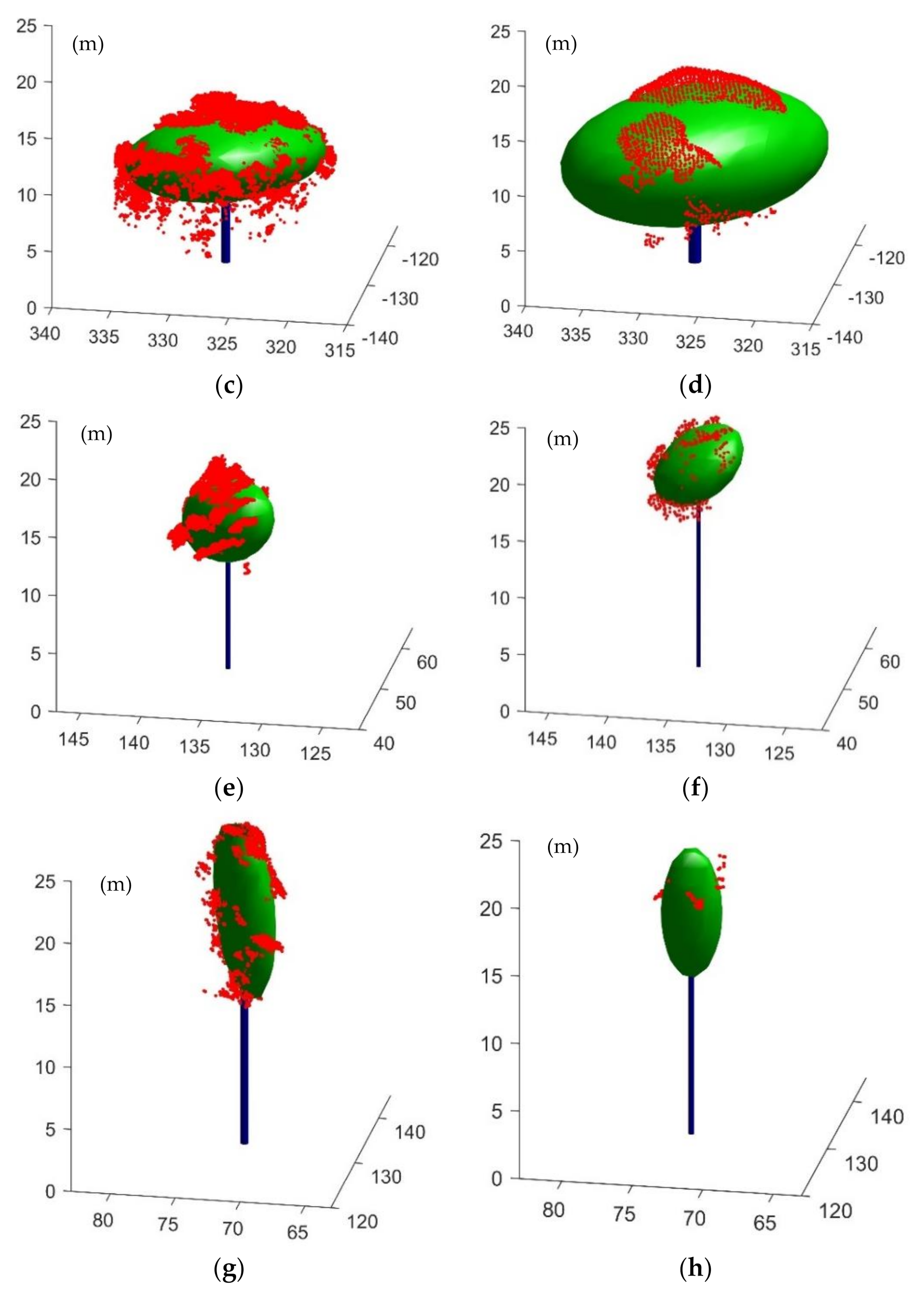
4.2. Point Clouds Fitting Result

In this study, four samples of the tree were modeled. The four samples have different characteristics. The first and second samples are trees that have a high-density canopy. The first tree sample has dense characteristics in the vertical direction, while the second sample has dense characteristics in the horizontal direction. The third and fourth tree samples are tall tree species but have a low-density canopy. The point clouds of all tree samples can be seen in Figure 8. The shape of the point clouds from LiDAR and photogrammetric data is almost the same for trees with high-density canopy, while for trees with low-density canopy, photogrammetric point clouds do not look like actual trees.

The R² value of the sphere fitting ranges from 0.002 to 0.029. This value is negligible and indicates that 3D modeling using the sphere fitting method is not recommended. This is because the sphere fitting cannot accommodate various canopy shapes. For example, in sample tree 1, the shape of the leaves that extends upward cannot be modelled. In addition, in the second tree model, in the form of the tree extending to the side, the resulting canopy model exceeds the lower limit of the formed trunk model, as seen in Figure 9.

The value of R² in 3D modeling of the individual tree using the ellipsoid fitting method is more diverse and has a wide range of values. In this method, the value of R² ranges from 0.338 to 0.952. This is because the ellipsoid fitting method is more flexible in making the canopy shape of the individual tree. The orientation and size of the model match the shape of the point clouds of the individual tree. In the program, there is an option to adjust the complexity of the resulting elliptical surface. The smaller the value of complexity, the fewer surfaces and vertices of the surface, and vice versa. However, this does not affect the value of R² made. The complexity value only affects the resulting visual model. The modeling results can be seen in Figure 10.

The spherical harmonics fitting method gives the highest average R² value compared to other fitting methods. The spherical harmonics method has an R² value between 0.324 to 0.945. The spherical harmonics method can shape the tree shape according to the canopy shape generated by the point clouds can be seen in Figure 11. However, what is lacking in this method is that there are a lot of vertices and faces generated on the surface, so it requires a long duration for data processing and also produces a reasonably large surface size when it is converted to CityGML format.

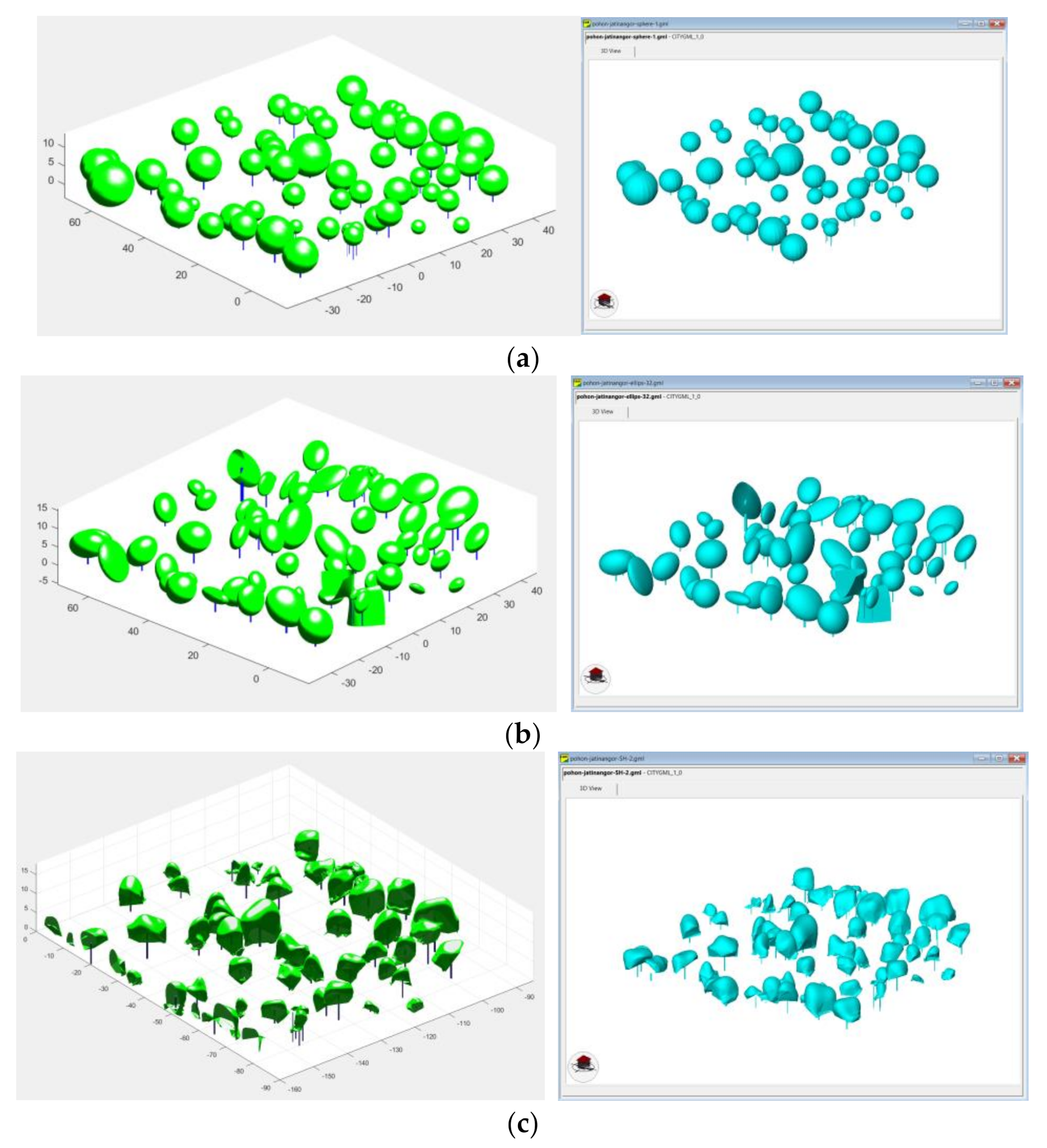
4.3. CityGML Conversion Result

Individual tree modeling is also carried out in the area of interest with 64 trees. The 3D modeling results of the individual tree in the area of interest region is then converted into CityGML format. The program generates a 3D model of LiDAR point clouds and photogrammetry on a surface. Surfaces are stored in faces and vertices matrices. The format of faces and vertices needs to be converted into an n × 12 matrix according to the multisurface format in CityGML, where n is the number of faces in the individual tree. Multisurface data is stored in the <gml:posList> section as a geometric representation of the tree for canopy and trunk sections.

The CityGML format can be opened in the FZK Viewer software. The results of 3D modeling in CityGML format can be seen in Figure 12.

4.4. Biomass Estimation

The calculation of AGB is carried out in the area of interest, which was modeled in the previous section. The estimation of AGB was obtained from DBH data derived from the tree crown radius. The value of the tree crown radius is obtained from each modeling method: sphere fitting, ellipsoid fitting, and spherical harmonics fitting. The value of the crown radius of the sphere fitting is obtained from the radius of the modelled sphere. In the ellipsoid method, the canopy radius value is obtained from the average flattening radius of the elliptical model. In the spherical harmonics method, the radius value is taken from the average distance of each point to the center of the canopy model. In this study, the allometric calculation of AGB uses Equation (15) from [37].

$$AG{B}_{EST}=0.066{\left(D\right)}^{2.59}$$

(15)

where D is the DBH in cm and $AG{B}_{EST}$ is the estimated Above-Ground Biomass. The biomass calculation was carried out on two datasets, namely data from UAV LiDAR point clouds and UAV photogrammetry point clouds data. The biomass calculation is based on the DBH value obtained from the canopy of the point clouds of UAV LiDAR and UAV photogrammetry. The calculations of the two methods were then validated using the results of DBH measurements in the field. The calculation of biomass using UAV LiDAR data with the sphere modeling method gives the results closest to the field validation value with an accuracy of 78%. Meanwhile, the method with the farthest calculation is the photogrammetric data approach using the spherical harmonics modeling method with an accuracy of 44%. Comparison of the results of biomass calculations using the UAV LiDAR method, UAV photogrammetry, and conventional method for field validation can be seen in

Table 4. The results of biomass calculations using the LiDAR method, photogrammetry, and conventional method.

Fitting Method	Above-Ground Biomass (Metric tons/ha)
	LiDAR	Photogrammetry	Field Validation
Sphere	22.157	64.127	28.423
Ellipsoid	21.084	65.610
Spherical Harmonics	20.161	65.946

.

5. Discussion

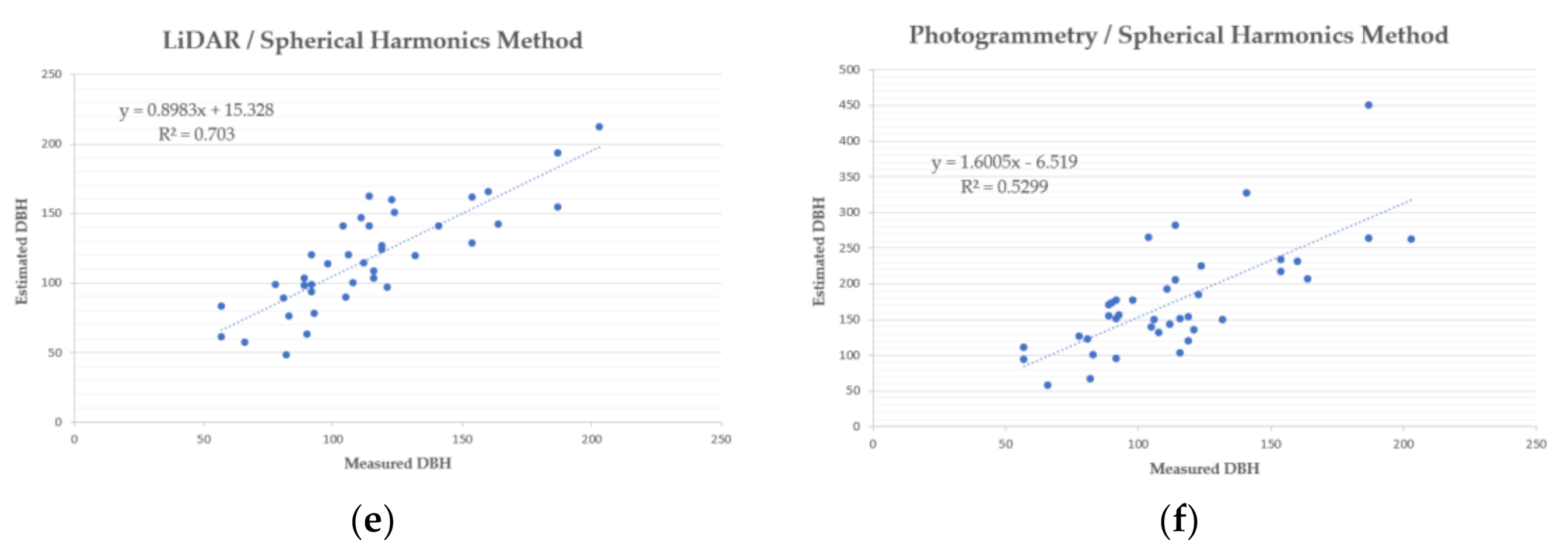
5.1. Diameter Breast Height (DBH) Estimation Analysis

The tree DBH is determined by using an allometric equation that looks at its relationship with the tree crown radius. The polynomial equation model gives the best results because it has the largest R² value among other equations. The R² value of the polynomial equation of 0.870 indicates that the tree crown has a strong relationship with the tree DBH from field measurement results. This illustrates that the model can estimate the trunk’s diameter as much as 87% based on the radius of the tree canopy, and other factors explain the remaining 13%. This is in line with research conducted by [46] that there is a strong relationship between the length of the diameter of the crown and DBH with an R² value of 0.778 using the polynomial equation. However, the difference is not very significant. The logarithmic equation has the worst R² value of all. This shows that the logarithmic equation cannot perform the regression between the diameter of the DBH and the tree crown radius.

In some studies, such as the research conducted by [47], the DBH value is directly obtained from the point clouds by using estimation methods such as Hough transform, RANSAC, and RTLS. These results give a bias of 0.1 cm with an RMSE of 6 cm. In this study, this method could not be used because of the low density of point clouds generated by LiDAR. The density obtained from point clouds in research [47] is 2000 points per m², while in this study, the density is only about 120 m² for LiDAR data, so the trunk section cannot be seen clearly. It can be seen in Figure 13, where the point clouds of the trunk cannot be seen clearly. This is due to differences in the LiDAR sensors used. In addition, the point clouds of the photogrammetry data only cover the tree canopy surface, and it is impossible to create point clouds from the trunk using the photogrammetric method. The method used in this paper is suitable for the type of LiDAR sensor that produces low-density point clouds.

In other studies, the photogrammetric method used to calculate DBH is the close-range photogrammetric method [48]. DBH calculation using the close-range photogrammetric method has a Root Mean Square Error (RMSE) value of 4.41 cm. However, the weakness of this method is that it is challenging to implement and requires a much longer time than the UAV photogrammetry method. As such, this research uses allometric equations to obtain the DBH value from each tree derived from the crown radius data from the tree.

5.2. D Reconstruction of Trees Analysis

The 3D modeling method using spherical harmonics fitting is the best compared to the sphere fitting and ellipsoid fitting methods when viewed from the average R² value and the resulting visual form. In general, the 3D modeling generated from LiDAR data is better than the 3D model generated by photogrammetry for each method. The point clouds generated by LiDAR data have a higher density and shape closer to the original object’s shape so that the resulting 3D model is even better. In addition, samples 1 and 2 of the tree have a higher R² value, and the model is closer to the actual shape than individual samples 3 and 4. Tree samples 1 and 2 have high-density canopy characteristics than samples 3 and 4. Tree with a high-density canopy produces more point clouds data. The low point clouds data causes the surface model of the canopy not to form.

However, the fitting process still has some drawbacks, such as the first, the lower part of the canopy is not well-formed, especially in modeling using photogrammetric point clouds. This is because the photogrammetric point clouds data is only a surface of the tree and only covers the center of the canopy. Modeling LiDAR data does not always produce a good bottom of the canopy. There are gaps between the canopy and the trunk so that the canopy seems to float. This is because the second tree sample has a very dense canopy so that the point clouds at the bottom cannot be acquired. It is complicated to fit the third and fourth tree types with the spherical harmonics fitting method. The lack of the point clouds data and the more random distribution make the modeling results visually poor and result in a smaller R2 value than the two previous tree samples.

In principle, the spherical harmonics method transforms point clouds resulting from UAV LiDAR and UAV photogrammetry data acquisition into a smoother form of a closed surface. The point clouds generated directly by UAV LiDAR are random and irregular, so the spherical harmonics method converts the data into point clouds data that form a more stable surface. The process of making a surface from point clouds data resulting from the spherical harmonics transformation is then carried out using various methods such as convex hull, concave hull, alpha shape, and robust crust. These methods produce different surfaces according to the algorithm of each technique. The results of the surface fitting can be seen in Figure 14 and Figure 15.

The convex hull and concave hull methods produce simpler data with fewer vertices and faces. This is because the convex hull and concave hull methods perform surface reconstruction only on the outermost part of the resulting point clouds. The surface formed by the concave hull and convex hull methods is nearly identical.

Alpha shape is a heuristic approach and performs well in uniform sampling. However, the optimal value of alpha is on the sampling density, which continuously changes at different parts of the surface [49]. In the alpha shape and robust crust methods, the form of the surface more closely follows the shape of the point clouds, which has implications for the number of vertices and a more significant number of faces. There are differences in the volume calculations generated from the surface from LiDAR data and photogrammetric data. Using LiDAR data, the resulting volume ranges from 600–700 m³, while photogrammetric data ranges from 800–900 m³. There is a significant difference because the point clouds produced by the photogrammetric method are only at the top of the canopy, so the model generated at the bottom of the canopy is not formed perfectly, resulting in a different modeling form from the surface generated from LiDAR data. The number of vertices, faces, and volumes generated for each surface reconstruction method can be seen in

Table 5. The number of vertices, faces, and volumes generated for each surface reconstruction method.

Surface Reconstruction Method	LiDAR Point Clouds			Photogrammetry Point Clouds
	Vertex	Faces	Volume (m3)	Vertex	Faces	Volume (m3)
Convex Hull	77,694	103,588	672.762	4644	6188	905.045
Concave Hull	77,754	13,668	726.935	4722	6292	902.132
Alpha Shape	117,981	157,304	627.068	4881	6504	852.709
Robust Crust	236,028	314,700	596.224	9732	12,972	824.963

.

In general, the robust crust method using LiDAR data is the best in performing surface reconstruction resulting from point clouds resulting from spherical harmonics transformations.

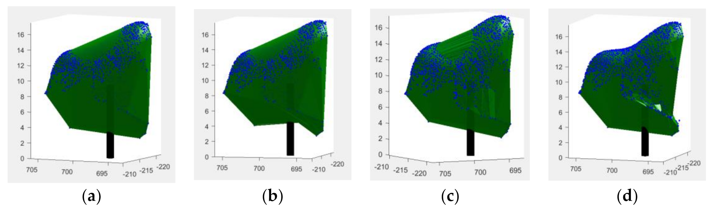
5.3. CityGML Conversion and Data Storage

Each fitting method has a different conversion time and the resulting data’s size. In the area of interest, with the device we used, the sphere fitting method takes 6 seconds to convert and produces CityGML data at 13 MB. The ellipsoid fitting method takes 24 s and has CityGML data at 64 MB. The spherical harmonics method, as the most complicated method, takes 350 s and produces a CityGML file with 500 MB.

Based on the modeling results, for visualization and analysis of green open space areas for an area that is not too wide or under 50 ha, the spherical harmonics fitting method can consider the conversion time and the size of the resulting data. Meanwhile, to conduct individual tree modeling in relatively large open green spaces or above 50 ha, the suitable method used is the sphere fitting method and the ellipsoid fitting. Considering that this method can quickly produce data in CityGML format, the data size is relatively small and can still be accommodated by computers with relatively low specifications.

Visually, the 3D model generated by the spherical harmonics method better describes the actual situation in the field. The ellipsoid fitting method produces a model with good visuals, but some trees have few point clouds, so the resulting 3D model does not form a perfect ellipse. This can be corrected by filtering or selecting which trees will be modelled. One of the filtering methods used is the wavelet analysis method performed by [50]. This method filters the point clouds data generated by the UAV photogrammetry method, which is considered to have much noise before modeling. Trees whose cloud data points are below the threshold can be ignored, and modeling is not carried out.

5.4. Above-Ground Biomass Estimation Analysis

The results of the biomass calculation show that measurements using UAV LiDAR data both using sphere, ellipsoid, and spherical harmonics modeling provide values that are closest to the results of field validation. Estimation of AGB value using UAV LiDAR data gives an accuracy in the range of 71–78% compared to the results of field validation, while estimation using photogrammetric data gives accuracy in the range of 43–44%. This is because the approximate value of the crown radius of each tree is more comparable to the actual field conditions than photogrammetric data. The photogrammetric data has a much greater value than the data from the field validation because several trees have a very large tree crown value which affects the estimated DBH value. An example of a very large tree crown value can be seen in Figure 16a, which is indicated by the letters A and B compared to Figure 16b, which is indicated by the letters A and B. There is a significantly huge difference in tree crown radius that causes the difference in the AGB value.

The estimated AGB value is largely determined by the DBH value derived from the allometric equation obtained in the previous section. The relationship between DBH values from field measurements and DBH estimates using the three modeling methods can be seen in Figure 17. There is a strong relationship when estimated DBH are calculated using UAV LiDAR data with the three aforementioned modeling methods. Each has an R² value of 0.706, 0.711, and 0.703. Estimated DBH value using the UAV photogrammetry data gives a more scatter graph and a smaller R² with a value of 0.539, 0.503, and 0.529.

The research shows that the closest estimation value for calculating the AGB value is the sphere fitting approach. AGB values range from 20–22 metric tons/ha for LiDAR UAV data and 61–62 metric tons/ha for photogrammetric UAV data. This is in line with the research conducted by [51], where the AGB value produced in one plot was 5.9 metric tons/ha for clove plants. Meanwhile, research [52] shows that the AGB value in tropical forests has an average of 98 metric tons/ha. The tree used as a sample in this study has a density greater than that of the study [51] and smaller than that of the study [52].

Several studies use different equations in calculating above-ground biomass as in research conducted by [53]. The study only used metrics from tree height to determine AGB with the following equation.

AGB = 555.2 + 6724.7 × Hmax + 4856.3 × Hmajority + 314.1 × Hvariety

(16)

In this study, DBH calculations were carried out because height calculations would be difficult to validate. This is because the trees in the area studied have a height in the range of 10–25 m, so it is complicated to conduct a field survey to obtain an appropriate and accurate height value.

5.5. Vizualization Validation

In addition, the modeling results are compared with the results of field photos visually. This is done to see the quality of modeling in one area of interest, which is done visually. Based on the results of the calculation of the value of R², the spherical harmonics method gives the best value, which means the modeling form is closest to the shape of the formed point clouds. In comparison with aerial photographs of the area of interest region, the modeling results from LiDAR are closer to the actual shape in the field than the photogrammetric method. The comparison can be seen in Figure 18.

The modeling results seen from above are then compared with the digitized results manually to see a 2D view of the modeling results. Based on the comparison results seen in Figure 19, modeling using photogrammetric data is not much different from using LiDAR data. As such, modeling using photogrammetric data can still be done for visualization purposes.

6. Conclusions and Suggestions

In this study, a 3D model of the individual tree in a green open space area was created in CityGML format. The proposed workflow carried out in this study starts from data acquisition, point clouds segmentation, surface fitting on point clouds, equation calculation to determine DBH, conversion to CityGML format, and AGB calculation. The acquisition was carried out using the UAV LiDAR and UAV photogrammetry methods.

In the segmentation section, this paper performs segmentation using the manual method. This will certainly be time-consuming if the area to be modeled is vast. Point clouds segmentation needs to be done automatically for segmentation on both orthophoto products and point clouds products. Segmentation can be done using machine learning or deep learning methods, which are currently being done in many other studies. The automatic tree classification method can be compared with the manual classification method to see the accuracy of the automated segmentation results.

Based on this research, the modeling results of the point clouds produced by LiDAR have a better accuracy value than the photogrammetric point clouds. The type of tree also influences the modeling accuracy. Trees with high-density canopy cover have better modeling accuracy than the low-density canopy. In addition, the surface fitting method affects the accuracy of the modeling. The spherical harmonics method provides better accuracy than the ellipsoid and sphere methods. However, the problem with modeling using the spherical harmonics method is that the processing time is relatively long and requires a sophisticated workstation. In addition, 3D data stored in CityGML format for the spherical harmonics method requires a very large storage size so that this method is suitable for landscape architectures whose area is relatively small. Meanwhile, modeling with the ellipsoid and sphere methods is suitable for large areas such as urban forests and vegetation in urban areas to perform specific analyses.

AGB calculation is much better using LiDAR data compared to photogrammetric data. This is indicated by the AGB value generated by the LiDAR data, which is closest to the field validation results compared to the photogrammetric data. In future works, another acquisition method with photogrammetry that can be used for further studies is using an oblique camera system with multiple sensors. In this system, many parts of the data can be retrieved compared to conventional methods so that the accuracy of the modeling can be improved. As such, it is hoped that the calculation of the AGB value using photogrammetric data can be more accurate.

References

1. Vitousek, P.M. Beyond global warming: Ecology and global change. Ecology 1994, 75, 1861–1876. [Google Scholar] [CrossRef]
2. Ribeiro, H.V.; Rybski, D.; Kropp, J.P. Effects of changing population or density on urban carbon dioxide emissions. Nat. Commun. 2019, 10, 3204. [Google Scholar] [CrossRef] [Green Version]
3. Jayawardena, A.W. Climate change—Is it the cause or the effect? KSCE J. Civ. Eng. 2015, 19, 359–365. [Google Scholar] [CrossRef]
4. Shi, A. Population growth and global carbon dioxide emissions. In IUSSP Conference in Brazil/Session-s09; The World Bank: Washington, DC, USA, 2001. [Google Scholar]
5. Kampa, M.; Castanas, E. Human health effects of air pollution. Environ. Pollut. 2008, 151, 362–367. [Google Scholar] [CrossRef] [PubMed]
6. Heidt, V.; Neef, M. Benefits of urban green space for improving urban climate. In Ecology, Planning, and Management of Urban Forests; Springer: New York, NY, USA, 2008; pp. 84–96. [Google Scholar]
7. Lubis, S.H.; Arifin, H.S.; Samsoedin, I. Analisis cadangan karbon pohon pada lanskap hutan kota di DKI Jakarta. J. Penelit. Sos. Ekon. Kehutan. 2013, 10, 1–20. [Google Scholar] [CrossRef]
8. Lessie, O.-C. Urban Vegetation Modeling 3D Levels of Detail. Master’s Thesis, Delft University of Technology, Delft, The Netherlands, 2018. [Google Scholar]
9. Yao, Z.; Nagel, C.; Kunde, F.; Hudra, G.; Willkomm, P.; Donaubauer, A.; Adolphi, T.; Kolbe, T.H. 3DCityDB—A 3D Geodatabase Solution for the Management, Analysis, and Visualization of Semantic 3D City Models Based on CityGML. Open Geospat. Data Softw. Stand. 2018, 3, 5. [Google Scholar] [CrossRef] [Green Version]
10. Biljecki, F.; Stoter, J.; Ledoux, H.; Zlatanova, S.; Çöltekin, A. Applications of 3D City Models: State of the Art Review. ISPRS Int. J. Geo-Inf. 2015, 4, 2842–2889. [Google Scholar] [CrossRef] [Green Version]
11. Konde, A.; Saran, S. Web enabled spatio-temporal semantic analysis of traffic noise using CityGML. J. Geomat. 2017, 11, 248–259. [Google Scholar]
12. Kavisha, K.; Ledoux, H.; Commandeur, T.J.F.; Stoter, J.E.; Kavisha, K. Modeling urban noise in CityGML ADE: Case of the Netherlands. In Proceedings of the 12th 3D Geoinfo Conference, Melbourne, Australia, 26–27 October 2017; p. 4. [Google Scholar]
13. Hajji, R.; Yaagoubi, R.; Meliana, I.; Laafou, I.; Gholabzouri, A.E. Development of an Integrated BIM-3D GIS Approach for 3D Cadastre in Morocco. ISPRS Int. J. Geo-Inf. 2021, 10, 351. [Google Scholar] [CrossRef]
14. Stojanovic, V.; Trapp, M.; Richter, R.; Hagedorn, B.; Döllner, J. Towards the generation of digital twins for facility management based on 3D point clouds. In Proceeding of the 34th Annual ARCOM Conference, Belfast, UK, 3–5 September 2018; pp. 270–279. [Google Scholar]
15. Singh, S.; Shrivastava, V.; Sharma, V. CityGML based 3D modeling of urban area using UAV dataset for estimation of solar potential. In Proceedings of the International Conference on Unmanned Aerial System in Geomatics, Roorkee, India, 6–7 April 2019; pp. 355–367. [Google Scholar]
16. Rosser, J.F.; Long, G.; Zakhary, S.; Boyd, D.S.; Mao, Y.; Robinson, D. Modeling urban housing stocks for building energy simulation using CityGML EnergyADE. ISPRS Int. J. Geo-Inf. 2019, 8, 163. [Google Scholar] [CrossRef] [Green Version]
17. Bao, K.; Padsala, R.; Thrän, D.; Schröter, B. Urban Water Demand Simulation in Residential and Non-Residential Buildings Based on a CityGML Data Model. ISPRS Int. J. Geo-Inf. 2020, 9, 642. [Google Scholar] [CrossRef]
18. Toschi, I.; Ramos, M.M.; Nocerino, E.; Menna, F.; Remondino, F.; Moe, K.; Fassi, F. Oblique photogrammetry supporting 3D urban reconstruction of complex scenarios. Int. Arch. Photogramm. Remote Sens. Spat. Inf. Sci. 2017, XLII-1/W1, 519–526. [Google Scholar] [CrossRef] [Green Version]
19. Jayaraj, P.; Ramiya, A.M. 3D Citygml Building Modeling from Lidar Point Cloud Data. Int. Arch. Photogramm. Remote Sens. Spat. Inf. Sci. 2018, XLII-5, 175–180. [Google Scholar] [CrossRef] [Green Version]
20. Popovic, D.; Govedarica, M.; Jovanovic, D.; Radulovic, A.; Simeunovic, V. 3D Visualization of Urban Area Using Lidar Technology and CityGML. In IOP Conference Series: Earth and Environmental Science; IOP Publishing: Bristol, UK, 2017; p. 95. [Google Scholar]
21. Ortega, S.; Santana, J.M.; Wendel, J.; Trujillo, A.; Murshed, S.M. Generating 3D city models from open LiDAR point clouds: Advancing towards smart city applications. In Open Source Geospatial Science for Urban Studies; Springer: New York, NY, USA, 2021; pp. 97–116. [Google Scholar]
22. Ledoux, H.; Biljecki, F.; Dukai, B.; Kumar, K.; Peters, R.; Stoter, J.; Commandeur, T. 3dfier: Automatic reconstruction of 3D city models. J. Open Source Softw. 2021, 6, 2866. [Google Scholar] [CrossRef]
23. Guo, Z.; Liu, H.; Pang, L.; Fang, L.; Dou, W. DBSCAN-based point cloud extraction for Tomographic synthetic aperture radar (TomoSAR) three-dimensional (3D) building reconstruction. Int. J. Remote Sens. 2021, 42, 2327–2349. [Google Scholar] [CrossRef]
24. Sharafzadeh, A.; Esmaeily, A.; Dehghani, M. 3D Modeling of Urban Area Using Synthetic Aperture Radar (SAR). J. Indian Soc. Remote Sens. 2018, 46, 1785–1793. [Google Scholar] [CrossRef]
25. Kolbe, T.H. Representing and exchanging 3D city models with CityGML. In 3D Geo-Information Sciences; Springer: Berlin/Heidelberg, Germany, 2009; pp. 15–31. [Google Scholar]
26. Biljecki, F.; Ledoux, H.; Stoter, J. An improved LOD specification for 3D building models. Comput. Environ. Urban Syst. 2016, 59, 25–37. [Google Scholar] [CrossRef] [Green Version]
27. Arroyo Ohori, K.; Biljecki, F.; Kumar, K.; Ledoux, H.; Stoter, J. Modeling Cities and Landscapes in 3D with CityGML. In Building Information Modeling; Springer: Cham, Switzerland, 2018; pp. 199–215. [Google Scholar]
28. Trisyanti, S.W.; Suwardhi, D.; Harto, A.B. 3D Landscape Recording and Modeling of Individual Trees. Hayati J. Biosci. 2019, 26, 185–195. [Google Scholar] [CrossRef]
29. Gobeawan, L.; Lin, E.S.; Tandon, A.; Yee, A.T.K.; Khoo, V.H.S.; Teo, S.N.; Poto, M.T. Modeling Trees for Virtual Singapore: From Data Acquisition to Citygml Models. Int. Arch. Photogramm. Remote Sens. Spat. Inf. Sci. 2018, XLII-4/W10, 42. [Google Scholar] [CrossRef] [Green Version]
30. Agus, M.; Veloz Castillo, M.; Garnica Molina, J.F.; Gobbetti, E.; Lehväslaiho, H.; Morales Tapia, A.; Calí, C. Shape analysis of 3D nanoscale reconstructions of brain cell nuclear envelopes by implicit and explicit parametric representations. Comput. Graph. X 2019, 1, 100004. [Google Scholar] [CrossRef]
31. Fan, G.; Nan, L.; Dong, Y.; Su, X.; Chen, F. AdQSM: A New Method for Estimating Above-Ground Biomass from TLS Point clouds. Remote Sens. 2020, 12, 3089. [Google Scholar] [CrossRef]
32. Wagers, S.; Castilla, G.; Filiatrault, M.; Sanchez-Azofeifa, G.A. Using TLS-Measured Tree Attributes to Estimate above Ground Biomass in Small Black Spruce Trees. Forests 2021, 12, 1521. [Google Scholar] [CrossRef]
33. Ten Harkel, J.; Bartholomeus, H.; Kooistra, L. Biomass and crop height estimation of different crops using UAV-based LiDAR. Remote Sens. 2020, 12, 17. [Google Scholar] [CrossRef] [Green Version]
34. Gonzalez de Tanago, J.; Lau, A.; Bartholomeus, H.; Herold, M.; Avitabile, V.; Raumonen, P.; Calders, K. Estimation of above-ground biomass of large tropical trees with terrestrial LiDAR. Methods Ecol. Evol. 2018, 9, 223–234. [Google Scholar] [CrossRef] [Green Version]
35. Walter, J.; Edwards, J.; McDonald, G.; Kuchel, H. Photogrammetry for the estimation of wheat biomass and harvest index. Field Crops Res. 2018, 216, 165–174. [Google Scholar] [CrossRef]
36. Gil-Docampo, M.D.L.L.; Arza-García, M.; Ortiz-Sánz, J.; Martínez-Rodriguez, S.; Marcos-Robles, J.L.; Sánchez-Sastre, L.F. Above-ground biomass estimation of arable crops using UAV-based SfM photogrammetry. Geocarto Int. 2020, 35, 687–699. [Google Scholar] [CrossRef]
37. Ketterings, Q.M.; Coe, R.; van Noordwijk, M.; Palm, C.A. Reducing uncertainty in the use of allometric biomass equations for predicting above-ground tree biomass in mixed secondary forests. For. Ecol. Manag. 2001, 146, 199–209. [Google Scholar] [CrossRef]
38. Yan, Z.; Liu, R.; Cheng, L.; Zhou, X.; Ruan, X.; Xiao, Y. A concave hull methodology for calculating the crown volume of individual trees based on vehicle-borne LiDAR data. Remote Sens. 2019, 11, 623. [Google Scholar] [CrossRef] [Green Version]
39. Trochta, J.; Krůček, M.; Vrška, T.; Král, K. 3D Forest: An application for descriptions of three-dimensional forest structures using terrestrial LiDAR. PLoS ONE 2017, 12, e0176871. [Google Scholar] [CrossRef] [Green Version]
40. Rachakonda, P.; Muralikrishnan, B.; Cournoyer, L.; Cheok, G.; Lee, V.; Shilling, M.; Sawyer, D. Methods and considerations to determine sphere center from terrestrial laser scanner point clouds data. Meas. Sci. Technol. 2017, 28, 105001. [Google Scholar] [CrossRef] [Green Version]
41. Brown, S. Estimating Biomass and Biomass Change of Tropical Forests: A Primer; Food and Agriculture Organization: Rome, Italy, 1997; Volume 134. [Google Scholar]
42. Sutaryo, D. Penghitungan Biomassa Sebuah Pengantar untuk Studi Karbon dan Perdagangan Karbon; Wetlands International Indonesia Programme: Bogor, Indonesia, 2009. [Google Scholar]
43. Kuyah, S.; Muthuri, C.; Jamnadass, R.; Mwangi, P.; Neufeldt, H.; Dietz, J. Crown area allometries for estimation of aboveground tree biomass in agricultural landscapes of western Kenya. Agrofor. Syst. 2012, 86, 267–277. [Google Scholar] [CrossRef]
44. Basuki, T.M.; Van Laake, P.E.; Skidmore, A.K.; Hussin, Y.A. Allometric equations for estimating the above-ground biomass in tropical lowland Dipterocarp forests. For. Ecol. Manag. 2009, 257, 1684–1694. [Google Scholar] [CrossRef]
45. Liu, K.; Shen, X.; Cao, L.; Wang, G.; Cao, F. Estimating forest structural attributes using UAV-LiDAR data in Ginkgo plantations. ISPRS J. Photogramm. Remote Sens. 2018, 146, 465–482. [Google Scholar] [CrossRef]
46. Iizuka, K.; Yonehara, T.; Itoh, M.; Kosugi, Y. Estimating tree height and diameter at breast height (DBH) from digital surface models and orthophotos obtained with an unmanned aerial system for a Japanese cypress (Chamaecyparis obtusa) forest. Remote Sens. 2018, 10, 13. [Google Scholar] [CrossRef] [Green Version]
47. Kuželka, K.; Slavík, M.; Surový, P. Very High Density Point cloudss from UAV Laser Scanning for Automatic Tree Stem Detection and Direct Diameter Measurement. Remote Sens. 2020, 12, 1236. [Google Scholar] [CrossRef] [Green Version]
48. Mokroš, M.; Liang, X.; Surový, P.; Valent, P.; Čerňava, J.; Chudý, F.; Tunák, D.; Saloň, Š.; Merganič, J. Evaluation of close-range photogrammetry image collection methods for estimating tree diameters. ISPRS Int. J. Geo-Inf. 2018, 7, 93. [Google Scholar] [CrossRef] [Green Version]
49. Yu, Y. Surface reconstruction from unorganized points using self-organizing neural networks. IEEE Vis. 1999, 99, 61–64. [Google Scholar]
50. Fryskowska, A. Improvement of 3D Power Line Extraction from Multiple Low-Cost UAV Imagery Using Wavelet Analysis. Sensors 2019, 19, 700. [Google Scholar] [CrossRef] [Green Version]
51. Harapan, T.S.; Husna, A.; Febriamansyah, T.A.; Mutashim, M.; Saputra, A.; Taufiq, A.; Mukhtar, E. Above Ground Biomass Estimation of Syzygium aromaticum using structure from motion (SfM) derived from Unmanned Aerial Vehicle in Paninggahan Agroforest Area, West Sumatra. J. Biol. UNAND 2021, 9, 39–46. [Google Scholar] [CrossRef]
52. Ota, T.; Ogawa, M.; Shimizu, K.; Kajisa, T.; Mizoue, N.; Yoshida, S.; Ket, N. Aboveground biomass estimation using structure from motion approach with aerial photographs in a seasonal tropical forest. Forests 2015, 6, 3882–3898. [Google Scholar] [CrossRef] [Green Version]
53. Maesano, M.; Khoury, S.; Nakhle, F.; Firrincieli, A.; Gay, A.; Tauro, F.; Harfouche, A. UAV-Based LiDAR for High-Throughput Determination of Plant Height and Above-Ground Biomass of the Bioenergy Grass Arundo donax. Remote Sens. 2020, 12, 3464. [Google Scholar] [CrossRef]
Figure 1. (a) The orthophoto of ITB Jatinangor Campus and (b) the modeling area of interest.
Ijgi 11 00174 g001
Figure 2. The point clouds data generated by (a) LiDAR and (b) photogrammetry.
Ijgi 11 00174 g002
Figure 3. The cross-section of the point clouds resulting from (a) LiDAR data acquisition and (b) photogrammetry data acquisition.
Ijgi 11 00174 g003
Figure 4. The results of the segmentation of the individual tree point clouds from (a) LiDAR data acquisition and (b) photogrammetry data acquisition.
Ijgi 11 00174 g004
Figure 5. The flowchart of proposed methodology.
Ijgi 11 00174 g005
Figure 6. The Scatter Plot of Relationship between Canopy Radius Estimated Value and DBH Value from Field Measurement Results.
Ijgi 11 00174 g006
Figure 7. The regression result of DBH estimation using (a) linear method, (b) polynomial method, (c) power method, and (d) logarithmic method.
Ijgi 11 00174 g007aIjgi 11 00174 g007b
Figure 8. Point clouds from (a) the first tree sample using the LiDAR method, (b) the first tree sample using the photogrammetric method, (c) the second tree sample using the LiDAR method, (d) the second tree sample using the photogrammetric method, (e) the third tree sample using the LiDAR method, (f) the third tree sample using the photogrammetric method, (g) the fourth tree sample using the LiDAR method, and (h) the fourth tree sample using the photogrammetric method. Table 3 shows the R2 value from each modeling carried out.
Ijgi 11 00174 g008
Figure 9. 3D model by sphere fitting method of (a) the first tree sample using the LiDAR method, (b) the first tree sample using the photogrammetric method, (c) the second tree sample using the LiDAR method, (d) the second tree sample using the photogrammetric method, (e) the third tree sample using the LiDAR method, (f) the third tree sample using the photogrammetric method, (g) the fourth tree sample using the LiDAR method, and (h) the fourth tree sample using the photogrammetric method.
Ijgi 11 00174 g009aIjgi 11 00174 g009b
Figure 10. 3D model by ellipsoid fitting method of (a) the first tree sample using the LiDAR method, (b) the first tree sample using the photogrammetric method, (c) the second tree sample using the LiDAR method, (d) the second tree sample using the photogrammetric method, (e) the third tree sample using the LiDAR method, (f) the third tree sample using the photogrammetric method, (g) the fourth tree sample using the LiDAR method, and (h) the fourth tree sample using the photogrammetric method.
Ijgi 11 00174 g010aIjgi 11 00174 g010b
Figure 11. 3D models by the spherical harmonics fitting method of (a) the first tree sample using the LiDAR method, (b) the first tree sample using the photogrammetric method, (c) the second tree sample using the LiDAR method, (d) the second tree sample using the photogrammetric method, (e) the third tree sample using the LiDAR method, (f) the third tree sample using the photogrammetric method, (g) the fourth tree sample using the LiDAR method, and (h) the fourth tree sample using the photogrammetric method.
Ijgi 11 00174 g011
Figure 12. Conversion result of tree model in Area of Interest for (a) spherical fitting, (b) ellipsoid fitting, and (c) spherical harmonics fitting method.
Ijgi 11 00174 g012
Figure 13. The red circle shows the trunk part of the three sample trees point clouds which is not clearly formed.
Ijgi 11 00174 g013
Figure 14. Surface reconstruction results on LiDAR point clouds that have been transformed by spherical harmonics fitting using (a) convex hull, (b) concave hull, (c) alpha shape, and (d) robust crust methods.
Ijgi 11 00174 g014
Figure 15. Surface reconstruction results on photogrammetric point clouds that have been transformed by spherical harmonics fitting using (a) convex hull, (b) concave hull, (c) alpha shape, and (d) robust crust methods.
Ijgi 11 00174 g015
Figure 16. Differences in tree crown radius from the modeling results of individual tree (A) and group of trees (B) with the sphere method on (a) photogrammetry data and (b) LiDAR data.
Ijgi 11 00174 g016
Figure 17. Scatter plot of measured DBH value from field validation with estimated DBH value (a) sphere modeling with LiDAR data, (b) sphere modeling with photogrammetric data, (c) ellipsoid modeling with LiDAR data, (d) ellipsoid modeling with photogrammetric data, (e) spherical harmonics modeling with LiDAR data, and (f) spherical harmonics modeling with photogrammetric data.
Ijgi 11 00174 g017aIjgi 11 00174 g017b
Figure 18. Comparison between the results of 3D modeling of trees using a spherical harmonics method on (a) photogrammetric data and (b) LiDAR data with the actual situation in the field visually.
Ijgi 11 00174 g018aIjgi 11 00174 g018b
Figure 19. Comparison between (a) manual tree digitization results with (b) top view of modeling with LiDAR data and (c) top view of modeling with photogrammetric data.
Ijgi 11 00174 g019