An Occupancy Information Grid Model for Path Planning of Intelligent Robots

Abstract

Commonly used robot map models include occupancy grid maps, topological maps, and semantic maps. Among these, an occupancy grid map is mainly represented as a quadrilateral grid. This paper proposes an occupancy information grid for intelligent robots by exploiting the advantages of the occupancy grid map and spatial information grid. In terms of geometric structure, a regular hexagonal grid is used instead of a regular quadrilateral grid. In terms of attribute structure, the single obstacle attribute is replaced by the grid terrain characteristics, grid element attributes, and grid edge attributes. Thus, the occupancy information grid model is transformed into a new data structure describing the spatial environment, and it can be effectively applied to map construction and path planning of intelligent robots. For the map construction application of intelligent robots, this paper describes the basic process of laser sensor-based grid model construction. For the path planning application of intelligent robots, this paper extends the A* algorithm based on a regular hexagonal grid. Additionally, map construction and path planning applications for intelligent robots are experimentally verified. Several experimental results were obtained. First, the experimental results confirmed the theoretical conclusion that the minimum sampling density of the hexagonal structure was 13.4% lower than that of the quadrilateral structure. Second, the regular hexagonal grid is clearly more advantageous in describing environmental scenes, which can ameliorate the "undercompleteness" phenomenon. Third, there were large differences in the planning paths based on two types of grids, as shown by the fact that the distance of the planning paths obtained by the regular hexagonal grid was reduced by at least 10.8% and at most 15.6% compared with the regular quadrilateral grid.

1. Introduction

With the continuous development of robotics, the use of maps is gradually shifting from humans to robots with data processing and cognitive capabilities. The robot actively acquires environmental information through its laser or vision sensors, forming a map model for describing its spatial environment [1].

The commonly used robot map models are classified as occupancy grid maps, topological maps, and semantic maps [2]. The occupancy grid map discretizes the spatial environment perceived by robots into equally sized grids and then applies a specific probability of occupation to assign the attributes of the grid [3]. The IEEE RAS Map Data Representation Working Group released a standard for 2-D maps in robotics [4]; the standard defines the main metric representation for planar environments to facilitate data exchange, benchmarking, and technology transfer. The topological map uses nodes and edges to describe the connectivity and topology of the spatial environment abstractly, and usually uses the generalized Voronoi diagram to express topological relationships, which is described as "a topological representation of a map that contains all the key information of the map and represents the intrinsic information in a more compact form" [5,6]. Compared to the occupancy grid map, it can only roughly represent the spatial environment [7]. The semantic map describes the spatial environment according to semantic concepts and processes each element in a categorical hierarchy, presenting a map to the robot in a similar manner to that in which people use maps [8]. It can use the conditional random field model [9], end-to-end deep learning architecture [10], probabilistic algorithm [11], or hierarchical semantic map framework [12] to generate semantic point clouds to achieve global modeling and semantic sharing of robot environments.

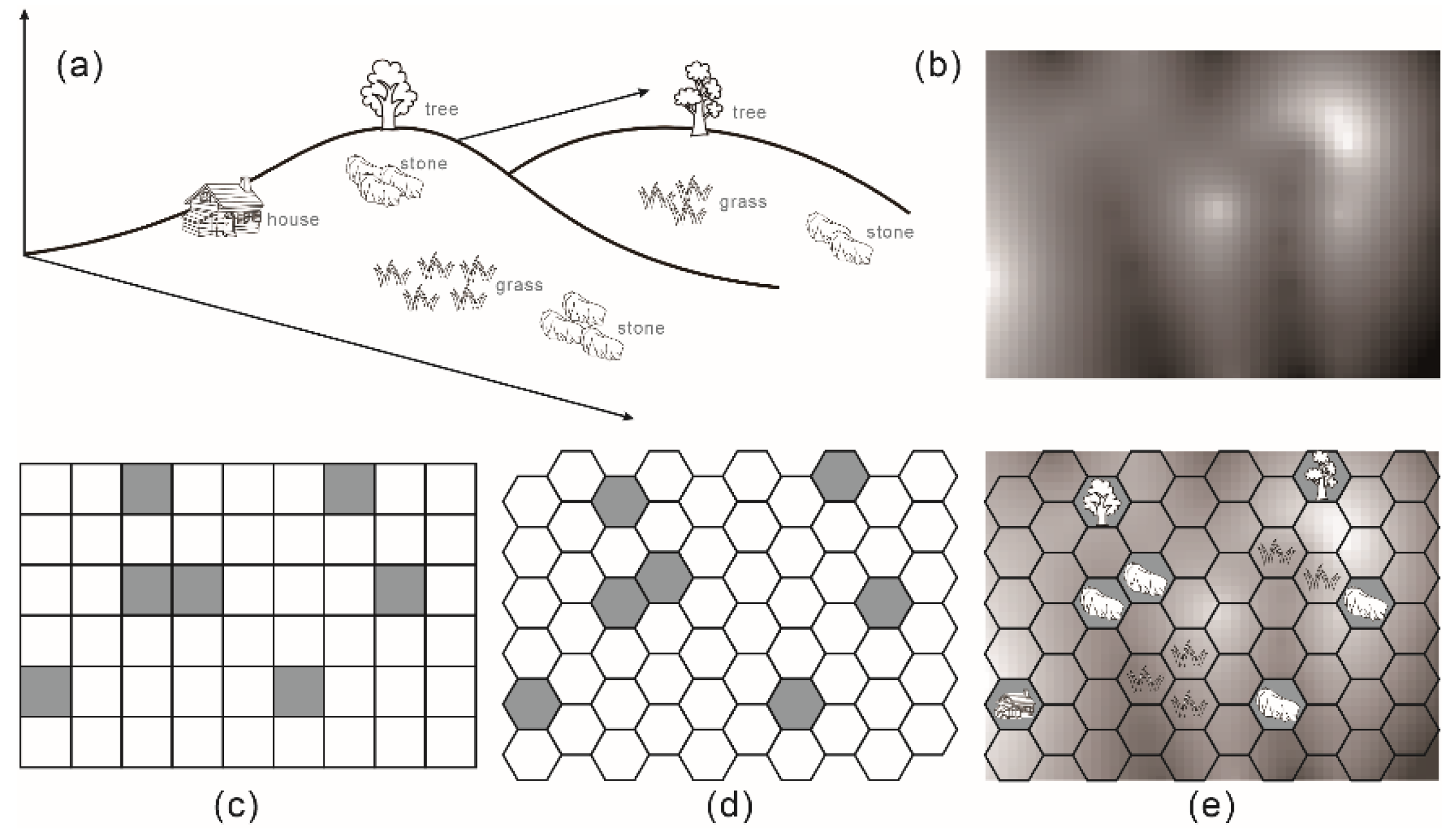
For practical use, the occupancy grid map is still the classic and most commonly used form of spatial environment representation. It generates a 2D, or 3D spatial environment model by using different sensors and assigns values such as 0 (idle), 1 (occupancy) or 2 (unknown) for robot path planning and real-time navigation (Figure 1c).

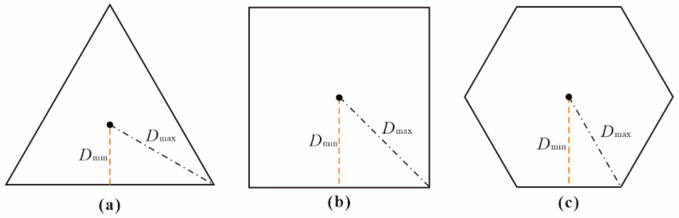
An occupancy grid map is essentially a grid model. According to the division characteristics of the discrete spatial grid, the hexagonal grid was found to be the best form of distribution of planar points. It has more consistent proximity, more isometric measurement directions, and higher angular resolution than the grids comprised of triangles and quadrangles. Therefore, it provides more accurate descriptions of locations and attributes in the spatial environment. Therefore, some researchers used the regular hexagonal grid instead of the quadrilateral grid to describe the spatial environment (Figure 1d), which is used as the data basis for robot path planning, for example, in the study by Quijano and Garrido [13]. In this paper, we construct a new map model applicable to robots, named an occupancy information grid model. Assuming that the robot explores the spatial environment, as shown in Figure 1a, and its relief is shown in Figure 1b, Figure 1c is a traditional occupied grid map, and Figure 1d is the occupancy grid map in the form of regular hexagons. Figure 1e is the occupancy information grid model. The occupancy information grid model expands the terrain characteristics, grid element attributes, and grid edge attributes. In this model, the hexagonal grid is used to discretize the spatial environment, the terrain factor is applied to describe the topographic undulations, and the grid element attributes, and edge attributes are used to represent the spatial area, and spatial obstacle features, respectively. The result is a map model suitable for robot path planning and real-time navigation. First, the paper describes the basic concept of the occupancy information grid model, which includes its geometric and attribute structure. Second, a detailed description is provided for the map construction algorithm of the robot-based occupancy information grid model, which involves the processes of grid occupation probability estimation, map updating, and map matching. Third, the A* algorithm is adapted to the occupancy information grid model, and then the path planning of robots is realized. Finally, this paper designs an experiment for a grid model construction and path planning to verify the rationality and feasibility of the occupancy information grid model in terms of the accuracy of environmental expression and path planning.

The three main contributions of this paper are as follows. First, the use of a more advantageous regular hexagonal grid instead of a regular quadrilateral grid makes the description of the spatial environment more reasonable. Second, the grid structure is used to extend the multiple expressions of the spatial environment, which involve terrain characteristics, grid element attributes, and grid edge attributes. This removes the limits on the occupancy grid map that are related to the expression of a single attribute and provides an innovative map model of robot cognition. Third, the A* algorithm for robot-oriented grids is extended to combine the cost constraints of the terrain characteristics, grid element attributes, and grid edge attributes to achieve a more complex and intelligent path planning algorithm.

2. Related Work

The occupancy grid map is essentially a description model of the spatial environment oriented toward robots.

A similar concept exists in the field of geographic information science, but with humans as the object of service. Grids are an alternative form of data organization corresponding to vector data structures called raster data models. The spatial environment is partitioned into regular grids, and each grid is assigned corresponding attribute values to represent spatial entity data that are ultimately used to describe the spatial environment. According to Chen et al., a grid map based on the raster data model is a relatively simple map type [14]. It divides the mapping area into grids according to plane coordinates or the latitude and longitude lines of the Earth. The attribute classification, statistical classification, and change parameters are described or expressed with the grid as a unit, which is equivalent to expressing the law of dynamic spatial and temporal changes in two-dimensional space. Therefore, the grid map based on raster data has strong adaptability and diversity. Li et al. proposed the concept of a spatial information multigrid from the perspective of urban management applications [15,16,17]. On global and national scales, there are grids of various grid sizes that correspond to the level of coarse or fine detail. Each grid is defined by the geographical location of its center point and records closely related basic data. However, their grids are irregular polygons corresponding to administrative regions, which is a strong limitation.

The grid in geographic information science is usually used as a basic model of the spatial environment for road design, emergency evacuation of people, flood simulation, and so on. Kraak and Ormling collected soil, groundwater, vegetation, animal populations, and geoheritage data in a regular grid to analyze the impact of high-speed railways on the above data and finally selected the best high-speed railway construction route from several possible routes [18]. Li et al. used a spatiotemporal grid model to manage and analyze the trajectory data, which is represented by spatiotemporal grid encoding instead of vector coordinates, and then reduced the computational complexity of the algorithms [19]. The spatial environment is an important factor affecting the simulation effect of emergency evacuation of crowds [20]. It not only directly affects the movement behavior of agents but also affects the visual effect of the simulation results. The spatial environment description of crowd emergency evacuation simulation draws on the form of cellular automata and is also expressed in the form of a grid [21]. Lai et al. integrated 3D topographic survey data and 2D building vector data, established an urban model based on a regular hexagonal grid, and realized the simulation of urban waterlogging and flooding [22].

Grid research in geographic information science provides another idea for this paper; that is, more attribute information can be used to fill the grid, instead of simply 0 (idle), 1 (occupancy), or 2 (unknown), and transform the occupancy grid map into an occupancy information grid. Meanwhile, the field of robotics has focused mostly on probabilistic localization, path planning, and automatic control rather than on map models used by robots. Quijano and Garrido used a hexagonal grid instead of a quadrilateral grid to simulate the exploration environment of a robot and analyzed the effects of the two grids on the search efficiency using several different path search algorithms [13]. Tao et al. addressed the shortcomings of traditional quadrilateral grids in environmental description and path planning, fully compared the construction process of traditional, rhombic, hexagonal, and triangular grids and studied the arrangement coding of hexagonal grids, and analyzed the motion indicators corresponding to different grids based on the octree strategy [23]. These studies are similar to our paper, but they focused on the difference formed by the geometric structure of the grid rather than the grid model. Li et al. analyzed the path planning efficiency of an unmanned surface vehicle during environmental monitoring [24]. They used hexagons to partition the sampling area and planning paths based on spanning tree planning. Their research has some implications for our paper, although they focused more on path planning than on the grid model.

This paper draws on the idea of dissecting spatial information grids and extends the traditional occupancy grid map in terms of the geometry and attribute structure of the grid to form a grid model suitable for robot cognition. The differences between the quadrilateral model and the hexagonal model in terms of environment description and path planning are also compared, and the rationality and feasibility of applying the hexagonal grid to robot maps are demonstrated.

3. Grid Model Structure

3.1. Geometric Structure

A geometric structure is a series of regular polygons covering a plane or a sphere that are continuous, seamless, and nonoverlapping to divide the spatial environment, determine spatial locations and describe spatial properties. Considering the specificity of the grid covering the study area, these regular polygons should satisfy at least two conditions. First, the distance from the polygon centroid to each edge is the same in all directions. Ideally, the distance is the same from the center point to the edges in all directions, i.e., a circle. However, a circle cannot be stitched continuously on a region; therefore, it is necessary to select a regular polygon instead of a circle for approximation. Second, the polygon must be a continuous and nonoverlapping tessellation graph on the region [25].

Based on the above two conditions, the geometry of the suitable polygon can be determined.

Suppose there exists a positive n-side shape; then, each interior angle $\Delta A$ is:

$$\Delta A=\frac{\left(n-2\right)}{n}\times {180}^{°}$$

(1)

If this shape can form a continuous, seamless, and nonoverlapping tessellation in a plane, it necessarily requires that each of the m positive n-sides has an interior angle at a point that covers the plane exactly. Therefore,

$$m\times \Delta A=m\times \frac{\left(n-2\right)}{n}\times {180}^{°}={360}^{°}$$

(2)

From Formulas (1) and (2), we can obtain:

$$m=\frac{2n}{\left(n-2\right)}=2+\frac{4}{\left(n-2\right)}$$

(3)

where m and n are integers, and n is 3, 4, or 6. Only three types of regular polygons fit the geometry of the grid model, namely, regular triangle, regular quadrilateral, and regular hexagonal. Theoretically, they can be used as the geometric structure of a grid model.

3.1.1. Grid Center Distance Analysis

The grid center distance is the distance from the grid centroid to the edge. The geometry of the grid model is usually approximated by a circle with an inscribed regular polygon. Obviously, the distance from the centroid to the edge is not uniform. The perpendicular distance from the grid centroid to one side of a polygon is the nearest center distance (D_min), which is also called the isometric direction, and the distance from the grid centroid to the vertex of a polygon is the farthest center distance (D_max). The ratio of the farthest center distance to the nearest is called the grid center distance error (Figure 2). In general, a near-ideal grid should have more isometric directions and smaller grid center distance errors than a nonideal grid.

The grid center distance analysis was performed separately for the regular triangle, regular quadrilateral, and regular hexagonal. The following results were obtained: ① The regular hexagonal has the most isometric directions (i.e., 6). This means that more directions can be chosen from the centroid of a grid, which leads to more reasonable experimental results. ② The grid center distance errors of the hexagonal (≈1.155) are smaller than those of the triangle (=2.000) and quadrilateral (≈1.414), and a smaller error means that more accurate approximation results can be obtained. Therefore, the regular hexagon is more advantageous.

3.1.2. Grid Sampling Density Analysis

The process of overlaying a suitable grid over the area and then determining the attribute information for each grid unit is similar to the process of creating a digital image which is referred to as digital image sampling. The density of grids within a certain range is called the grid sampling density.

Assuming that the Fourier transform of a continuous two-dimensional image results in the shaded part in Figure 3a, the frequency band of the signal is in a circular region of radius $W$ in the frequency domain. The spectrum of the signal after the continuous band-limited image passes through a positive quadrilateral sampling grid is shown in Figure 3b. The sampling interval in the horizontal direction is $T_1$, the sampling interval in the vertical direction is $T_2$, and the sampling interval satisfies the Nyquist sampling theory, $T_1\le \frac{2\pi }{2W}$,$T_2\le \frac{2\pi }{2W}$.

The arrangement of the spectrum of the sampled signal in the frequency domain space is determined by the sampling matrix. The sampling matrix of a positive quadrilateral grid is the diagonal matrix V.

$$V=\left[\begin{array}{cc}{T}_1& 0\\ 0& T_2\end{array}\right]=\left[\begin{array}{cc}\frac{\pi }{W}& 0\\ 0& \frac{\pi }{W}\end{array}\right]$$

(4)

Figure 3a shows that the area of space occupancy by the hexagon outside the circle is smaller than that of the quadrilateral. The spectrum of the signal formed after the continuous image signal has been sampled by a positive hexagonal sampling grid satisfying Nyquist’s sampling theorem is shown in Figure 4a. The sampled signal spectrum has a much tighter spatial arrangement in the frequency domain than in the case of a positive quadrilateral sampling grid. The spatial sampling interval is determined by two directional vectors v₁ and v_2, as shown in Figure 4b, and the sampling matrix V consists of 2 directional vectors v₁ and v₂.

$$V=\left[\begin{array}{cc}{v}_1& v_2\end{array}\right]=\left[\begin{array}{cc}{T}_1& T_1\\ T_2& -T_2\end{array}\right]$$

(5)

The sampling grid in Figure 3 is a hexagon, so that of $T_2=\sqrt{3}{T}_1$. Since the spectrum of the continuous signal is in a circular region of radius $W$, to satisfy the Nyquist sampling theorem, $T_2\le \frac{2\pi }{2W}$, the sampling matrix of the hexagon is Formula (6).

$$V=\left[\begin{array}{cc}\frac{\pi }{\sqrt{3}W}& \frac{\pi }{\sqrt{3}W}\\ \frac{\pi }{W}& -\frac{\pi }{W}\end{array}\right]$$

(6)

The sampling density is the reciprocal of the determinant of the sampling matrix. Thus, comparing Formula (4) and Formula (6) proves that the minimum sampling density using a hexagonal structure is 13.4% lower than that for a positive quadrilateral structure [26].

Therefore, the hexagonal grid is selected for the intelligent robots proposed in this paper, and the differences in the quadrilateral grid and the hexagonal grid are compared.

3.2. Attribute Structure

The occupancy information grid model makes full use of the geometric structure to store attribute information. When each grid has different attribute information, the ensemble forms a conceptual model of the spatial environment. This is the key point that differentiates the grid model proposed in this paper from the occupancy grid map and spatial information grid. The grid model contains three types of attribute information. First, the terrain characteristic is used to describe the topographic undulations within the area occupancy by each grid. Second, the grid element attribute is used to describe the main spatial environment elements in the area occupancy by each grid (G in Figure 5). For example, is the dominant element a lake, inhabited land, or vegetation? Third, the grid edge attribute usually describes the adjacency relationship between neighboring grids. For example, a grid edge attribute of uncrossable rivers indicates that the current grid cannot cross this edge to reach adjacent grids, as shown in Figure 5 for A, B, C, D, E, and F. The attribute information of this grid model mainly comes from map data, and the terrain characteristic, grid element attributes, and grid edge attributes can be used as the database for real-time modeling to better serve the path planning applications of intelligent robots.

The most important manifestation of grid attributes is the cost value that is consumed by the robot. The traditional path planning algorithm takes the distance of the robot’s path as the cost value. When the cost value is the smallest, the shortest path planning of the robot is obtained. However, if the influence of terrain characteristics and surface elements on the robot’s motion is considered, then different terrain characteristics and different grid element attributes will affect the speed of the robot’s motion, resulting in different time consumption. The sum of the cost value through different grids is calculated; when the calculated value is the smallest, the optimal path is obtained.

3.2.1. Terrain Characteristics

Generally, the terrain characteristics of a grid use topographic factors to describe the topographic undulations within an occupancy area of each grid. Florinsky classified topographic factors as microscopic and macroscopic factors according to their computational characteristics [27]. Microscopic factors include slope, slope direction, plane curvature, etc.; macroscopic factors include average slope, surface cut depth, topographic relief, etc. Since the hexagonal grid usually occupies a certain area, Zhang selected the average slope or topographic relief as terrain factors [28]. In this paper, we also select the average slope to describe topographic undulations.

3.2.2. Grid Element Attributes

A grid element attribute is the value of a geographic element that occupies the dominant role in the spatial extent covered by a grid, which is similar to the raster map using RGB or gray values. According to the role of the grid element attribute, it is considered to be either an occupancy-type or indicator-type grid element.

The occupancy-type grid element is the primary element occupying an area. That is, the grid occupies a certain spatial range, and then the element occupying the largest area, the primary position, or the most important position is taken as the grid element attribute [29]. The occupancy-type grid element necessarily highlights the important elements and ignores secondary elements, thus generalizing the spatial environment. Two examples are the forest grid element (Figure 6a) and the city grid element (Figure 6b).

The indicator-type grid element is a special element that does not contain enough spatial elements to constitute occupancy grid elements. However, due to their extreme importance, they must be alienated from occupancy-type grid elements. In this paper, this type of grid element is referred to as an indication-type grid element to distinguish it from the occupancy-type grid elements. For example, the traffic element that has an important influence on robot motion is given the attribute of a grid element, such as a railroad (Figure 6c), even though it is expressed as a line element. Even if a grid has already been given the attribute of occupancy type, it can be superimposed on the original attribute to highlight the traffic information. Traffic information is defined as an indicative grid with distinct traffic characteristics, e.g., major roads in the city.

3.2.3. Grid Edge Attributes

The grid edge attribute takes full advantage of the geometry of the grid model, which is a distinctive feature that distinguishes it from other models, such as raster maps. Depending on the role of the grid edge attribute, it is characterized as an obstacle-type grid edge or an occupancy-type grid edge.

The obstacle-type grid edge is used to describe the pass and break relationship between two adjacent grids, e.g., whether it is possible to move through the edge from the current grid to the adjacent grid, such as the impassable river (Figure 6d).

The occupancy-type grid edge is relatively simple and depends on the obstacle-type grid edge, which is equivalent to superimposing another attribute on top of the obstacle-type grid edge to represent the additional information on top of the original grid edge. For example, rivers, as the main obstacle to pass, become the main source of obstacle-type grids. However, in the case of rivers, there are bridges above the rivers, and they are no longer obstacle grids because of the bridges.

For the spatial environment description, the terrain characteristic describes the undulating changes in a spatial environment, and the grid element attribute describes the point and surface elements, some of the line elements, and the grid edge attributes describe the line elements, which together define the basic framework of the conceptual model of a spatial environment. A large number of seamless, continuous nonoverlapping grids, with accompanying attribute information, together form the basic spatial environment. For path planning by intelligent robots, the terrain characteristics, grid element attributes, and grid edge attributes play their own distinct roles. Intelligent robots are affected by the slope, and as the complexity increases, they pay more cost to pass through the grid. The grid element attribute determines the different costs that a robot consumes when passing through a grid with specific properties. This is similar to the grid with different soils, where the cost to pass through a hard soil grid element is less than the cost relative to loose soil. It can then cause t intelligent robots to travel a farther distance.

The grid edge attributes determine whether they can cross the grid to reach the adjacent grid, similar to the rivers, steep hills, and washes. This has a certain hindering effect on robot motion only when the performance of the robot exceeds the limit of rivers, steep hills, or washes; otherwise, it may hinder their movement.

4. Grid Model Construction

Map data and laser sensors are two main sources for modeling occupancy information grid models for intelligent robots. Map data, the main way to describe the spatial environment, provides the basic data source. Laser sensors can provide highly representative point cloud data, which are suitable for real-time modeling and rapid updating of grids. In practical use, laser sensors can be used to build a grid, and the real-time modeling and rapid updating of a grid can be achieved based on the basic grid constructed by map data and point cloud data obtained from the laser sensors.

According to the basic grid constructed based on map data, the relative position coordinates of the robot, and the plane right angle coordinates of the laser point, the basic process of constructing the regular hexagonal grid model based on the laser sensor is shown in Figure 7.

First, based on the map data and grid size, a basic grid model is constructed, including the establishment of the geometric structure, as well as the terrain characteristics, grid element attributes, and grid edge attributes assigned to a grid model according to the map elements. This process is called a grid model constructed based on map data. However, here it is not fully described how to fill the grid with map data. Therefore, only a simple description of the geometric modeling of the grid, that is, the basic grid generated in this step, is a blank grid. Second, according to the coordinates of robots and the laser point, their coordinates in the grid model are determined, and the probability estimate of a grid where the laser point is located is calculated by applying the hidden Markov model. The Bresenham algorithm is used to update the state of the other grids between two grids. Finally, a map matching algorithm is applied to build the grid model of the spatial environment incrementally.

4.1. Grid Geometric Modeling

The geometric modeling of the grid model must specify the size, start point, orientation, and other information. As shown in Figure 8, the grid size is the distance H between opposite sides of the hexagonal grid, the grid start point is the lower-left corner point, and the grid orientation is the grid edge facing north [30].

Each hexagon of the grid model can be considered as an independent unit that stores uniformly encoded attribute information and interacts independently with the robot. Each hexagon contains both grid elements and grid edges. Therefore, the geometric modeling of the grid model essentially determines the coordinate values of each point and each edge of a hexagon, where the edges are identified as A, B, C, D, E, and F, and the points are identified as 1, 2, 3, 4, 5, and 6, as shown in Figure 5.

Suppose the center point coordinates of the lower-left hexagon are O(X₀,Y₀) and the grid size is H. Then, the center point coordinates in row i and column j can be calculated by formula (7), and the coordinates of each point can be calculated by formula (8).

$$\{\begin{array}{ll}{X}_{i,j}=\frac{\sqrt{3}}{2}H\left(j-1\right)+X_0\hfill & \hfill \\ Y_{i,j}=H\left(j-1\right)+Y_0\hfill & \left(j\%2\ne 0\right)\hfill \\ Y_{i,j}=H\left(j-1\right)+Y_0+\frac{H}{2}\hfill & \left(j\%2=0\right)\hfill \end{array}$$

(7)

According to the grid dissection algorithm, all of the point coordinates of the grid model are generated using the information of grid size and starting point coordinates to implement the grid dissection of the grid model in the whole plane area.

$$\{\begin{array}{cccc}{X}_1=X_{i,j}+\frac{\sqrt{3}}{6}H& Y_1=Y_{i,j}+\frac{1}{2}H& X_2=X_{i,j}+\frac{\sqrt{3}}{3}H\hfill & Y_2=Y_{i,j}\hfill \\ X_3=X_{i,j}+\frac{\sqrt{3}}{6}H& Y_3=Y_{i,j}-\frac{1}{2}H\hfill & X_4=X_{i,j}-\frac{\sqrt{3}}{6}H\hfill & Y_4=Y_{i,j}-\frac{1}{2}H\hfill \\ X_5=X_{i,j}-\frac{\sqrt{3}}{3}H& Y_5=Y_{i,j}& X_6=X_{i,j}-\frac{\sqrt{3}}{6}H\hfill & Y_4=Y_{i,j}+\frac{1}{2}H\hfill \end{array}$$

(8)

4.2. Probability Calculation

Grid modeling for intelligent robots essentially belongs to the simultaneous localization and mapping (SLAM) process that generally uses a probabilistic approach to represent the probability of the robot state at a certain moment in time. Assuming that the state information of the robot at moment $t$ is ${\mathit{x}}_t$, control information is ${\mathit{u}}_t$, and sensor measurement information is ${\mathit{z}}_t$, the robotic system solves for two main probabilities: the state transfer probability $p\left({\mathit{x}}_t|{\mathit{x}}_{t-1},{\mathit{u}}_{1:t}\right)$ and measurement probability $p\left({\mathit{z}}_t|{\mathit{x}}_t\right)$ [31].

The odometer detects control quantities such as linear and angular velocities of the robot in real-time while determining the robot’s pose information at the current moment based on the state information of the previous moment. The laser sensor scans the surrounding environment at a specific frequency to obtain measurement information, which is used for the construction of the grid model.

Assuming that the robot poses are known, the grid model is constructed to solve the problem of how to generate consistent maps based on the measurement data with noise and uncertainty. The grid model uses a series of binary random variables to represent the map, and the values of binary random variables indicate whether the current position is idle or occupied by an obstacle. Thus, the map construction process is the process of calculating the posterior probability $p\left(m|x_{1:t},z_{1:t}\right)$ of the whole map based on the given positional and measurement information.

4.3. Map Update

The process of map updating is to determine the grid through which the link passes and to estimate the state of the corresponding grid based on the linkage between the grids where the robot is located and any grid with a determined state. This process is updated using the Bresenham algorithm for the quadrilateral grid and requires a specific processing algorithm for the hexagonal grid.

Assume that the robot’s position is $\left(x_R,y_R\right)$, and the corresponding grid serial number is $\left(i_R,j_R\right)$ according to the regular hexagonal grid. The coordinate returned when the sensor scan line encounters an obstacle is $\left(x_S,y_S\right)$, and the corresponding grid serial number is $\left(i_S,j_S\right)$. The probability of occupancy by an obstacle is determined by a probability calculation algorithm [31]. Once the probability that grid $\left(i_S,j_S\right)$ is occupied by an obstacle is determined, the occupation (or idle) status of the other grids through which the scan line passes can be determined based on the robot’s position, coordinates, and grid serial number returned by the sensor scan line.

The grid determination method can be adapted to a regular hexagonal grid by a simple modification of the Bresenham algorithm (Figure 9); the steps are as follows:

① Calculate the rectangular range consisting of the grid $\left(i_R,j_R\right)$ and $\left(i_S,j_S\right)$, marked as $\left(X_{\min },Y_{\min }\right)$,$\left(X_{\max },Y_{\max }\right)$.

② Divide the rectangular area with equal spacing in $X_{\mathrm{dis}}=\frac{H}{2}$ and $Y_{\mathrm{dis}}=\frac{\sqrt{3}H}{6}$ and form a series of subgrids in a rectangle (Figure 9a).

③ Regularize the rectangular subgrids to make them square (Figure 9b).

④ Then, the grid determination based on a regular hexagonal grid through which the scan line passes can be implemented using the Bresenham algorithm.

⑤ When the horizontal subgrid number $I\%3\ne 0$, the regular hexagonal grid is searched backward from the subgrid number in the positive direction, and it can be determined that it is the grid that the scan line passes through, which belongs to the idle status.

⑥ When the horizontal subgrid number $I\%3=0$, we can use “the judgment method of points on the left or right side of a line” [28] to determine whether $\left(x_R,y_R\right)$ and $\left(x_S,y_S\right)$ are on the left or right side of the line segments B, C, E, and F in the regular hexagonal grid (Figure 5). If $\left(x_R,y_R\right)$ and $\left(x_S,y_S\right)$ are both on the left side of the line segment, then this grid is excluded; otherwise, it can be determined that it is the grid that the scan line passes through, which belongs to the idle status.

4.4. Map Matching

Probability estimation and map updating solve the problem of constructing a map of a robot when it is at a fixed position. As the robot keeps moving, the probability values of all grids are updated continuously, so that different grid models with the same resolution must be stitched together continuously by incremental map building until a complete grid model is formed.

The computer stores each grid of the grid model as a matrix, and each matrix element corresponds to a grid so that the complete environmental grid model corresponds to a pixel of the matrix. Assuming that the robot builds the grid model ${\mathrm{Map}}_G$ and ${\mathrm{Map}}_W$ at different moments with overlapping areas, it is necessary to stitch them together to incrementally build the environmental grid model. First, the edge pixels are extracted from grid models ${\mathrm{Map}}_G$ and ${\mathrm{Map}}_W$ using an edge extraction algorithm to form the edge pixel point sets, $G={\left\{g_i\right\}}_{i=1}^{N_g}$ and $W={\left\{w_i\right\}}_{i=1}^{N_w}$, where $g_i$ and $w_i$ are vectors and $N_g$ and $N_w$ denote the number of elements of the edge pixel point sets $G$ and $W$, respectively. The set of the edge pixel points in the overlap region of the grid model ${\mathrm{Map}}_G$ and ${\mathrm{Map}}_W$ is denoted by $G_{\epsilon }$, and is a subset of $G$ and $W$. The overlap percentage is denoted by $\epsilon$. Then, the incremental map building problem of the grid model at different moments is transformed into an image alignment problem by computing the rigid body transformation $T=\left\{R,t\right\}$ of the robot so that the point set $T\left(G\right)$ after the transformation process can be well matched with the point set $W$. In turn, the incremental map building problem of the grid model is expressed as a minimization problem:

$$\begin{array}{c}min\\ R,t,\epsilon ,G_{\epsilon }\\ f\left(i\right)\in \left\{1,2\dots N_w\right\}\end{array}\frac{1}{\left|G_{\epsilon }\right|{\left(\epsilon \right)}^{1+\lambda }}{\displaystyle \sum }_{P_i}{\left|\left|R{g}_i+t-w_{f\left(i\right)}\right|\right|}_2^2$$

(9)

where $\lambda$ is the control parameter and $|·|$ represents the minimum overlap percentage of the number of elements in the set, which is expressed by ${\epsilon }_{\min }$. Through continuous updating and matching, the incremental construction of the robot’s grid model is completed gradually, and finally, a complete grid model is formed.

5. Path Planning Algorithm Based on the Hexagonal Grid Model

Path planning is a key technology for autonomous robot navigation, which starts from the starting point and follows the path that is shortest, least time-consuming, and safe, and avoids collisions with all obstacles to the endpoint [32]. The path planning of robots can be mainly divided into global path planning and local path planning. Global path planning is implemented based on cost maps; the A* algorithm, the most widely used and influential heuristic graph search algorithm, uses a cost function to determine the values of the vertices in a path. If the cost function appears to be the optimal path, then this path is adopted. The closer the estimated value of the cost function is to the actual target value, the better the match between the cost function and the path. The estimated value function of the A* algorithm is:

$$f\left(n\right)=g\left(n\right)+h\left(n\right)$$

(10)

where $f\left(n\right)$ is the cost function to guide node expansion and search related to the time searching for the path with the smallest $f\left(n\right)$ between the start-point $S$ and end-point $E$; $g\left(n\right)$ is the path cost from the start-point $S$ to current node $n$; and $h\left(n\right)$ is the estimated path cost from the current node $n$ to end-point $E$. In the A* algorithm, $g\left(n\right)$ represents the actual distance that has been determined, and the optimal path can only be obtained if the value of $g\left(n\right)$ is guaranteed to be less than or equal to the actual consumption cost from the current node $n$ to end-point $E$ [33,34].

The A* algorithm is applied to a regular hexagonal grid; then, a grid is equivalent to a node, and a node can be connected to the surrounding six nodes [35]. To implement the heuristic A* algorithm, we have to preprocess the grid map and set some parameters. First, a cost table $T_{\cos \mathrm{t}}\left(i,j\right)$ based on the terrain characteristics and grid element attributes of each grid is created that represents the cost that a robot must spend to pass a grid. For terrain characteristics, if the average slope of the current grid is greater than the robot’s climbing ability, it indicates that the cost of the current grid is $+\infty$ (Figure 10a). A lower cost corresponds to a better path. A cost of $+\infty$ means that the robot cannot pass the grid. Second, an obstacle table $T_{\mathrm{obstacle}}\left(i,j\right)$ is built according to the grid edge attributes of each grid. This indicates that the robot cannot enter the adjacent grid from the current grid (Figure 10b). Third, Open, Closed, and Cost lists are created. The Open list stores the information from the current grid $G\left(i,j\right)$ to be checked, and its structure is $\left\{i,j,i_{parent},j_{parent},g,h,f\right\}$. In this structure, $i_{parent}$ and $j_{parent}$ represent the coordinates of the parent grid of $G\left(i,j\right)$, and put the start-grid $S$ into the Open list. The Closed list stores the grid that does not need to be examined again, and its structure is $\left\{i,j\right\}$. When initializing the Closed list, add the grid of ${\mathit{T}}_{\mathit{c}\mathit{o}\mathit{s}\mathit{t}}\left(\mathit{i},\mathit{j}\right)=\mathbf{0}$ and ${\mathit{T}}_{\mathit{o}\mathit{b}\mathit{s}\mathit{t}\mathit{a}\mathit{c}\mathit{l}\mathit{e}}\left(\mathit{i},\mathit{j}\right)=\mathbf{0}$ to the Closed list. The Cost list is used to check the viability of the adjacent grid in real-time and its structure is $\left\{i,j,g,h,f\right\}$, which represents the coordinate of the current grid and the actual value, heuristic value, and estimated value of its corresponding evaluation function. It should be emphasized that the algorithm revised in this paper is still an offline path planning algorithm.

Given the start-grid S and end-grid E, the heuristic A* algorithm flow for generating the optimal path based on a regular hexagonal grid is:

① Calculate the evaluation function of the start-grid and put it into the Open list.

② Check whether the Open list is empty. If it is empty, the path search fails, and the algorithm exits. Otherwise, proceed to the next step.

③ Judge whether the current grid is an end grid. If it is the target grid, go to step ⑦. Otherwise, go to the next step.

④ Compare the Closed list, and add the grid with $T_{cost}\left(i,j\right)=1$ to the Cost list. At the same time, calculate the corresponding $g$, $h$ and $f$ of the grid.

⑤ Update the Open list. Check the passable adjacent grid $G\left(i_{adjacent},j_{adjacent}\right)$ of the current grid $G\left(i,j\right)$ in the Cost list, and determine whether $G\left(i_{adjacent},j_{adjacent}\right)$ is in the Open list. If it is not, add $G\left(i_{adjacent},j_{adjacent}\right)$ to the Open list. Otherwise, determine the $f_{adjacent}$ value of $G\left(i_{adjacent},j_{adjacent}\right)$ in the Open list and the Cost list. If the $f_{adjacent}$ value of the Cost list is larger, add $G\left(i_{adjacent},j_{adjacent}\right)$ to the Open list. If the $f_{adjacent}$ value of the Open list is larger, update the parent grid in the Open list and update the corresponding $g$, $h$ and $f$ of the grid.

⑥ Determine the grid with the smallest value of $f$ in the Open list. If it is the end-grid, proceed to the next step. If it is not the end grid, set this grid as the current grid, calculate the $g$, $h$ and $f$ values in the Open list, add this grid to the Closed list, and return to step ③.

⑦ According to the grid and parent grid in the Closed list, starting from the end grid and backtracking to the start grid according to the parent pointer, the shortest path is determined.

6. Experimental

6.1. Experimental Design

6.1.1. Experimental Purpose

The purpose of this experiment was to verify the feasibility of the occupancy information grid model and the effectiveness of intelligent robot path planning. First, we constructed a quadrilateral grid and a hexagonal grid. We compared the abilities of two grids to describe the on-site environment from the perspective of modeling accuracy, and we studied the relationship between the scale of source data and the grid size used for grid modeling from the perspective of modeling scale. Second, we established a passage topology network based on a grid model and studied the feasibility of two grids in describing the planned paths from the perspective of navigation accuracy, i.e., the distance of each path based on its length and consistency with robot motion. The planned path is the path that is shorter and more consistent with the robot’s motion.

6.1.2. Experimental Environment

The experimental environment was selected from EFC Live Square in Hangzhou Future Science and Technology City (Figure 11a). The figure shows that EFC Live Square has a passage in the shape of an inverted C with stores on both sides. Different sizes of square quadrilateral and square hexagonal grids are modeled (Figure 11b,c).

6.1.3. Experimental Platform

Autolabor is used as the experimental platform [36]. This robot is equipped with a KINECT V2 camera, an AH-100B inertial measurement unit, and a Rplidar A2 LiDAR (its equipment parameters are shown in

Table 1. Device parameters of Rplidar A2 LiDAR.

Item	Attributes
Measuring radius	0.2–16 m
Sampling frequency	8 K
Angle resolution	0.9°
Ranging resolution	≤1% of actual distance (range ≤ 12 m)
	≤2% of actual distance (range ≈ 12 m–16 m)
Ranging accuracy	1% of actual distance (range ≤ 3 m)
	2% of actual distance (range ≈ 3 m–5 m)
	2.5% of actual distance (range ≤ 5 m–16 m)

). The three sensors are connected to Autolabor in a solid connection mode (Figure 12).

6.1.4. Experimental Steps

To achieve the above-described purpose of the experiments, the designed experimental steps were as follows.

Step 1: The EFC Live Square in Hangzhou Future Science and Technology City was selected as the experimental environment.

Step 2: The mobile robot equipped with RPLIDAR A2 radar was used to obtain the distance and angle information of the laser scanning points. Two types of grids were built with sizes in 0.1 m increments spanning the range of 0.1 m to 2 m.

Step 3: The passage area (10001) and four obstacle areas (20005, 20006, 20007, 20008) in Figure 15 were selected as the research objects. The two grid models were evaluated in terms of their abilities to describe the present environment from the perspective of modeling accuracy through graphical comparison and area statistics. Additionally, the effects of changing the grid size were analyzed.

Step 4: The start-grid and end-grid for path planning were defined, the A* algorithm was applied to conduct robot path planning based on the square quadrilateral and square hexagonal grids with different grid sizes, and the different paths planned by two grids were studied from the perspective of navigation accuracy.

6.2. Map Modeling Accuracy Analysis

The results obtained with the quadrilateral grid and hexagonal grid of EFC Live Square in Hangzhou Future Science and Technology City are shown in Figure 11.

First, the hexagonal grid had more grids than the quadrilateral grid (

Table 2. The number of grids in the experimental area.

ID	10001	20005	20006	20007	20008
True value of area (/m2)	2440.57	37.59	17.19	39.78	41.57
The number of grids when the grid size is 0.5 m	9761	150	67	159	167
	11279	175	79	184	193
	13.5%	14.3%	15.2%	13.6%	13.5%
The number of grids when the grid size is 1 m	2437	38	18	40	41
	2823	44	20	46	47
	13.7%	13.6%	10.0%	13.0%	12.8%
The number of grids when the grid size is 2 m	609	10	4	10	9
	702	10	6	11	11
	13.2%	0%	33.3%	9.1%	18.2%

). This indicates that the density of the hexagonal grid was higher than that of the quadrilateral grid. The experimental results show that the minimum sampling density of the hexagonal structure was 13.4% lower than that of the quadrilateral structure, except for the experimental area, which was too small (and the grid size was relatively too large) to reflect the real situation. Therefore, the hexagonal grid is clearly more advantageous than the quadrilateral grid in describing environmental objects and can ameliorate the "undercompleteness" phenomenon.

Second, as the grid size decreases, the grid more closely resembles the real scene, and there is little difference between the descriptions of the real scene provided by the grids. The details of the four obstacle areas (20005, 20006, 20007, 20008) shown in Figure 13 are good examples. Any grid is an approximate description of the environment, and the approximations of the visualization and the degree of the area depend on the grid size. There is no absolute criterion to determine which of two grids with the same size is superior.

However, when the size is large, the grid may still have some differences in describing the real scene. This difference is manifested in the delayed arrival of inaccurate descriptions due to the larger density of the hexagonal grid. For example, the T-shaped subchannel region (Figure 14) in the middle of the channel region (10001) is clearly not accurately described by the quadrilateral grid, resulting in the formation of two disconnected subregions, but is accurately described by the hexagonal grid.

Similarly, in the L-shaped subchannel region (Figure 14) in the upper part of the channel region (10001), both the quadrilateral grid and hexagonal grid obviously cannot accurately describe the environment. At the visual level, it appears that the square quadrilateral grid is closer than the square hexagonal to the real environment shape. However, there is essentially no difference between the experimental results obtained with the two grids for the path planning application.

The main reason for this is the same as discussed above, i.e., the hexagonal grid has a larger grid density, which leads to the delayed arrival of inaccurate descriptions.

Finally, the extent to which the area of the five experimental regions approximates the true value is analyzed for different grid sizes. The variable Q is constructed such that:

$$Q=\left|\frac{A_{grid}-A_{true}}{A_{true}}\right|\times 1000‰$$

(11)

where $A_{grid}$ is the area of the experimental region calculated based on the grid at different grid scales, and $A_{true}$ is the true value of the experimental region. The variable Q eliminates the effect of the scale on the experimental results. With the grid size as the x-axis and the variable Q as the y-axis, the experimental results are shown in Figure 15 and Figure 16.

The experimental results show that the area of the experimental area based on the grid calculation gradually converged to the true value as the grid size decreased, and relative equilibrium was reached when the grid size was less than 1.0 m. That is, when the grid size was 1.0 m and 0.1 m, the difference between the generated grids was very small. Thus, a larger grid size can be used instead of a smaller grid to balance the computational efficiency with the same modeling accuracy.

For a larger experimental area, for example, the channel area (10001), the deviation of the grid area from the true value was very small, only 5‰ when the grid size was 1.2 m, and not more than 2% when the grid size was 2.0 m. These results again verified that as the grid size decreased, the grid became closer to the real scene, and there was no significant difference between the different types of grids in describing the real scene. Smaller experimental areas were more sensitive to the changes in the grid size (Figure 16). However, in most cases, the deviation rate reached 5% when the grid size was 1.0 m. The small size of experimental areas caused them to be more sensitive to the grid size, but it also indicates that these smaller experimental areas may account for a smaller proportion of the whole current experimental area, or they should be among the objects to be sampled and removed for the current scale.

6.3. Navigation Accuracy Analysis

Above, the differences between two grids in describing an environment were analyzed from the perspective of modeling accuracy. The experimental results show that there is no significant difference between the two grids in terms of truth approximation; however, the hexagonal grid had a larger grid density than the quadrilateral grid of the same size, leading to a larger number of grids in the same area range and resulting in a more detailed global description of the environment and edges.

Here, the advantages, disadvantages, and rationality of path planning based on two grids were investigated from the perspective of navigation path accuracy. The start-point and end-point in Figure 11a were used as the start-grid and end-grid of robot path planning that was carried out using the A* algorithm based on the orthogonal quadrilateral grid and hexagonal grid with different grid sizes.

For path planning based on the quadrilateral grid, when the grid size changes from 0.1 m to 2.0 m, the planned path always showed the same trend by crossing the middle of the obstacle areas numbered 20005 and 20006, then moving south to the corner with the T-shape, and finally moving east to the end-grid (Figure 17a,b). This should be related to the fact that the quadrilateral grid specifies four directions of movement because there are no northeast, northwest, southwest, or southeast directions of movement. The A* algorithm tends to choose paths that are straight up and down or straight left and right.

For path planning based on the regular hexagonal grid, when the grid size changed from 0.1 m to 2.0 m, the planned path mostly approached gradually along the direction where the end-grid was located (Figure 17d); at a partial grid size, the planned path went around the obstacle area numbered 20006 and then approached gradually along the direction where the end-grid was located (Figure 17e). It appears that the experimental results were still in accordance with the expectations of the algorithm itself when path planning was performed based on both grids. The experimental results were always in accordance with the nature of the grid model regardless of which grid was used. Therefore, the experimental results were reasonable for both grids and depended on the grid size.

Second, as the grid size increased, the optimal paths could not be obtained from path planning based on the quadrilateral grid when the grid size was 1.8 m and 2.0 m, mainly because there was a topological road disconnection at the T-shape. However, this never occurred in the hexagonal grid because the density of the quadrilateral grid was smaller than that of the hexagonal grid. Clearly, as the grid size is increased, the T-shape disconnection eventually occurs, but it occurs later for the hexagonal grid with a more advantageous density than for the quadrilateral grid.

Finally, there is a large difference between the planning paths based on two grids, as shown by the fact that the planning paths obtained from the search of the grid model based on the hexagonal shape show a minimum reduction in the distance of 10.8% and a maximum reduction of 15.6% compared to the quadrilateral grid (

Table 3. Comparison of planning path length based on the different grid models.

Grid Size (/m)	Path Length with Quadrlateral (/m)	Path Length with Hexagonal (/m)	Reduction Ratio (%)	Grid Size (/m)	Path Length with Quadrilateral (/m)	Path Length with Hexagonal (/m)	Reduction Ratio (%)
0.1	70.0	60.5	13.6	39.78	1.1	70.4	60.5
0.2	70.0	60.4	13.7	70.0	1.2	70.8	61.2
0.3	69.9	60.6	13.3	69.9	1.3	70.2	61.1
0.4	70.4	60.0	14.7	70.4	1.4	70.0	60.2
0.5	70.5	61.0	13.5	70.5	1.5	70.5	61.5
0.6	70.2	60.6	13.7	70.2	1.6	72.0	60.8
0.7	70.7	60.9	13.9	70.7	1.7	71.4	62.9
0.8	69.6	60.8	12.6	69.6	1.8	/	61.2
0.9	71.1	61.2	13.9	71.1	1.9	70.3	62.7
1.0	71.0	62.0	12.7	71.0	2.0	/	62.0

). This is a very important conclusion! This means that the robot can travel less (by more than 10%), and the hexagonal grid can effectively improve the efficiency of path planning, reduce the path planning length, and thus reduce the accumulated error, enabling the robot to complete all of its tasks more accurately and efficiently while it is in motion.

6.4. Grid Attribute Impact Analysis

According to the previous description, the important feature of an occupied information grid model is to eliminate the single attribute of the occupied grid map and to expand the terrain characteristic, grid element, and grid edge attributes of each grid. Terrain characteristics, grid elements, and grid edge attributes affect path planning through different cost values.

In the path planning experiment of the A* algorithm based on the regular hexagonal grid, it is assumed that all grid costs use the path length as a standard. Then, the cost value of the robot passing through all grids is the same, so that the shortest path length is the path with the least cost, which is the optimal path, as shown in Figure 17e. We perform three simulation experiments for the grid surrounded by the ellipse in Figure 18a to analyze the influence of the grid attribute on the planned path, as follows:

(1) Grids are assigned grid elements with different cost values. As shown in Figure 18b, the grid element attribute is determined to be a forest. In the path planning experiment, it is reasonable to assume that the path length through the grid becomes twice the original length.

(2) The grid is given an average slope value greater than the robot’s ability to climb. As shown in Figure 18c, the average slope of the middle grid is 30°, and the surrounding grids are between 10° and 20°. Obviously, the robot cannot reach the middle grid from the surrounding grids.

(3) The upper-left edge of the grid is given an impassable river. As shown in Figure 18d, this indicates that the robot cannot enter the upper-left grid from the middle grid or cannot enter the middle grid from the upper-left grid.

The experimental results show that the planned paths calculated by the three simulation experiments and the grids passed by the original paths have changed, as shown in Figure 17g–i. The planned path length obtained from the three simulation experiments is still 62 m, showing that although some grids on the original route have undergone various changes, the A* algorithm based on the regular hexagonal grid can still find the optimal path. A detailed analysis of the grid whose properties have changed shows that the planned path is effectively avoided, indicating that the grid attributes indeed affect the A* algorithm, and the corresponding processing has been performed well.

7. Conclusions

This paper proposes an occupancy information grid model for intelligent robots.

The main contributions of this work include the following: ① A regular hexagonal grid is used to replace the traditional regular quadrilateral grid, and the differences between the two grids are theoretically analyzed in terms of the grid center distance and grid sampling density. ② The attribute expression of the grid model is expanded, and three contents of terrain characteristics, grid element attributes, and grid edge attributes are added, making the regular hexagonal grid a data model instead of a dissection algorithm. ③ The A* algorithm is expanded to make it applicable to regular hexagonal grids. At the same time, some conclusions were drawn through experiments. First, the density of the hexagonal grid was higher than that of the quadrilateral grid, and the experimental results confirmed the theoretical conclusion that the minimum sampling density of the hexagonal structure is 13.4% lower than that of the quadrilateral structure. Second, as the grid size decreased, the grid more closely described the real scene. There was no meaningful difference between the descriptions of the real scene obtained with different types of grids. However, the hexagonal grid was clearly more advantageous in describing the environmental objects, which could ameliorate the incomplete description of the environment by the grid. Third, there were large differences in planning paths based on two grids, as shown by the fact that the distance of the planning paths obtained from the search of the hexagonal grid was reduced by at least 10.8% and at most 15.6% compared with that of the quadrilateral grid.

In summary, it is reasonable and feasible to introduce the hexagonal grid in robot mapping applications and construct a new robot map model by expanding the terrain characteristics, grid element attributes, and grid edge attributes in hexagonal grids.