Digitalization and Classification of Cesare Battisti’s Atlas of 1915

Abstract

The paper deals with an automated methodology for the digital acquisition of thematic information from historical maps in order to use them for spatial analysis in a GIS software. This methodology has been applied to an early XIX c. map in order to assess the historical changes in the forest coverage in Trentino. Specifically, a tailored Object Based Image Analysis (OBIA) and filtering procedure has been applied to digitize and georeference Cesare Battisti’s map of forest density published in his atlas “Il Trentino. Economic Statistical Illustration” from 1915. According to the historical ecology approach, forest history can be analyzed and evaluated with the use of historical documentary sources. Following this approach, historical cartography is a precious information tool, and in many respects unique, through which it is possible to reconstruct the evolution of the forest cover of a given territory. Trentino, in particular, has a rich heritage of historical maps from which to draw useful information for the construction of a qualitative and quantitative diachronic picture of the evolutionary dynamics of wooded areas. In these territories, forest management is a topic of great importance both for its socio-economic implications and for the more strictly environmental ones, connected to the increasingly urgent need to implement mitigation and adaptation policies towards climate change. Thus, the paper presents the historical maps and illustrates the methodology used for the digitisation. Data extracted by the historical sources have been compared with the current one in order to identify changes in forest density in the last century.

1. Introduction

Historical maps are available in many countries and regions of the world and represent a valuable source of information in many fields [1,2]. Depending on the purpose for which the maps were designed and the period in which they were created, historical maps can be reliable in terms of precision and spatial accuracy [3], so they can usually be compared with modern maps not only to make qualitative assessments but also to quantify the changes occurred in time [4]. For example, in ecological studies it is widely recognized that past land use affects the distribution and status of current biodiversity [5,6,7,8], the provision of ecosystem services [9], and traditional ecological knowledge [10]. To be used in a Geographic Information System (GIS), historical maps must be digitized, georeferenced, classified, and possibly processed to filter out unwanted features [11]. The digitization of historical maps is usually done manually by one or more operators who essentially redraw the boundaries of the map and assign a conventional code to each feature, which is a long, time-consuming, and error-prone task [4,12]. Therefore automatic or semi-automatic procedures are necessary, especially when dealing with a large dataset and small scale research. A description of the challenges in the automatic classification of printed maps can be found in [11,13]. The approach used in the application described in this paper follows the procedure described in [14], with the use of additional texture and high pass filter bands to differentiate between different hatching patterns.

The historical cartographic source used is the “Boschi” (Woodland) map, produced by Cesare Battisti, and printed in the book “Il Trentino. Cenni geografici, storici, economici. Con un’appendice sull’Alto Adige” (“Trentino. Geographical, historical, economic notes. With an appendix on South Tyrol”) published in 1915 by the Istituto Geografico De Agostini in Novara, Italy.

For a long time, Cesare Battisti (1875–1916) has been remembered only because of his central role in the political and interventionist debate prior to the First World War and for his participation in the conflict. Nevertheless, more recently his figure has been re-evaluated as a pioneering scholar and expert on geography and territory [15,16]. Born in 1875 in Trento, a city belonging to the Habsburg Empire, Battisti moved to Florence, where he attended courses at the Istituto di Studi Superiori. In the Tuscan city, the geographer Giovanni Marinelli (1846–1900) had inaugurated a new tradition in the studying and teaching of geography that profoundly influenced the thought of the young man. In 1987, the same Marinelli was the supervisor of Battisti’s degree thesis devoted to the geography of Trentino. The thesis was one of the first monographic studies concerning an Italian region, analysing its physical-natural, historical, statistical-economic and demographic features, in order to provide an integrated and unified image of the territory, according to the theoretical perspective of the so-called “integral region” of the Florentine geographic school [17]. The following year, the work was published as a book in Trento [18].

After returning in Trento in 1900, Battisti focused energetically on the political commitment, initially as a militant of the Trentino Socialist Party, later as councillor of the Municipality of Trento, and finally as a deputy in the Parliaments of Vienna and Innsbruck [19]. Despite the preference given to the civil activities, Battisti did not totally leave his scientific and research interest in the geography of Trentino: between 1898 and 1914 he published at least 20 articles in local or national geographic journals, dedicated to a wide range of issues concerning Trentino territory. These papers updated and developed the data already collected for his thesis. Among the various themes, some of the studies focused on the problems and potential of local forest resources [20], and on the state of pastures, grazed woodlands, livestock, and the dairy industry [21]. These studies were also functional to Battisti’s public activity, as he was used to cite data, statistics, and studies to denounce the situation and to support his political proposal in all his public speeches.

In 1911, because of the failure of the Austro-Hungarian socialism and of the oppositions to Trento local autonomy claims, Battisti began to plead the annexation of Trentino to the Kingdom of Italy. In 1914 he was one of the most prominent exponents of the front favourable to the war between the Empire and Italy. In May 1915, coherently with his political positions, Battisti enlisted in the Italian Army and was sent to the front lines [19].

The publication project of the volume that collects Battisti’s published maps was developed in this context. The publisher Giovanni de Agostini offered Battisti the opportunity to publish an atlas to illustrate the Trentino territory to the general public in Italy. The result is a thematic atlas, composed of 62 pages of text and 19 colour maps, published in the autumn of 1915.

According to Marinelli’s approach, the regional analysis was based on the study of the spatial distribution of individual phenomena or elements, such as climate, flora, or demography, which were examined together to compose an overall picture to characterise the integral territorial context [22]. It is an educational and popular work aiming to provide an integral description of the Trentino region made more effective through the extensive use of cartography, and also to enhance local economic resources. Hence, the interest in forest resources, which, according to Battisti, guarantee an income of over 4,200,000 crowns per year; as specified in the book, “forestry is managed rationally in all the Trentino valleys, and especially in the valley of Fiemme, famous for the quality of the woods” [23].

The 19 colour maps illustrate a wide range of different aspects of regional geographical analysis [24]. The order of publication follows their quotation in the narrative chapters. The “Boschi” map, at a scale of 1:500,000, shows the theme of forest areas overlapped on the Carta d’Italia printed by the Italian Military Geographic Institute. For each administrative district of the Trento area, a series of symbols (that combine chromatic scale and dots) indicates the percentage of wooded area out of the total surface. The data are taken from the statistics of the Hapsburg Cadaster of XIX c. integrated with the reports of the Forest Districts of the Empire administration.

The analysis of Cesare Battisti’s scientific production can therefore represent a fundamental contribution to the history of geographical thought [15] but is also an interesting opportunity for applied historical cartography new tools and methodologies experimentations [25].

The aim of this study is to set up a procedure for the automatic classification of this type of historical maps, implemented using exclusively Free and Open Source Software (FOSS) systems. The application has been developed in GRASS GIS [26] and R [27], with specific GRASS add-on modules developed by the authors [14]. GRASS GIS is the leading GIS Free and Open Source Software (FOSS), used in research [28,29,30] and education [31]. R [27] is the most advanced environment for statistical computing and graphics, providing the modules for the classification using Machine Learning.

The paper is organized as follows: Section 2 describes the maps and the procedures used for the map classification: Section 2.1 outlines the map features and its historical importance, Section 2.3, Section 2.4 and Section 2.5 illustrate the segmentation and classification procedures, including the use of texture and high pass filters to detect different types of hatching patterns. Section 3 reports the results of the tests, with Section 3.1 describing the filtering methods and their outcome and Section 3.2 illustrating the procedures for the map geo-referencing. The use of the resulting map to assess the forest density change in the last century in Trentino is described in Section 3.4. Finally, the conclusions and future developments are presented in Section 4.

2. Materials and Methods

The map used for the procedure is the “Boschi” (Woodland) map available as an appendix of the book “Il Trentino. Cenni geografici, storici, economici. Con un’appendice sull’Alto Adige” by Cesare Battisti, published in 1915 by the Istituto Geografico De Agostini in Novara, Italy. The scale of the original maps is 1:500,000, with a pre-Rome40 datum and unprojected lat/long coordinates.

It is available as a digital image, but it is not georeferenced and it must be classified and filtered to create a map suitable for further processing. Therefore, a specific procedure has been created to classify, filter, and geo-reference the map.

2.1. Materials

Grounding on Annales school’s solicitations, international historiography started to approach the history of forests and woodlands from the 1950s. In the 1980s, forest history was a fully recognized branch of research, mainly devoted to analysing the relationship between wooded areas and human society [32]. Gradually, new research themes are emerging, as the relations between woodland and borders, ethnobotanics studies, as well as innovative application of GIS and Monoplotting software for the analysis of land use and coverage changes [33]. Actually, international scholars have agreed in the interpretation of forest and woodlands as historical products, deeply influenced during time by societies’ uses, managing and exploitation both in their ecology and their location and extension in the space. Indeed, if wooded areas are considered historical objects, they would be studied using classical historical sources, such as textual documents, photos, and maps, compared with field sources whenever possible [34,35].

Following this wake, the digital analysis of Cesare Battisti’s woodland map of 1915 can bring new light to the history of wooded areas in Trentino. These documents contain information on local forestry consistence in a fundamental moment of transition in the history, during the passage from Hapsbusrg Empire (and Hapsburg Forestry Laws) to the Italian Kingdom (and the Sardinian Foresty Code and, later, the Fascist Laws). Moreover, it makes available a new quantitative layer of forest spread and incidence dated between the already-known Hapsburg Cadaster (1853–1861) and the Carta forestale del Regno d’Italia (1936) [4,36].

The original book is comprised of 62 text pages and 19 colour maps, included as separate (folded) sheets [24]. It is available digitally in PDF format for text and JPEG for colour maps. The scanning resolution is 72 DPI, with unknown JPEG compression quality factor. Different sheets have different sizes because some of them cover the whole Trentino Alto Adige region, while other maps cover only part of the region, typically a province. Therefore, also the number of pixels is different for different images.

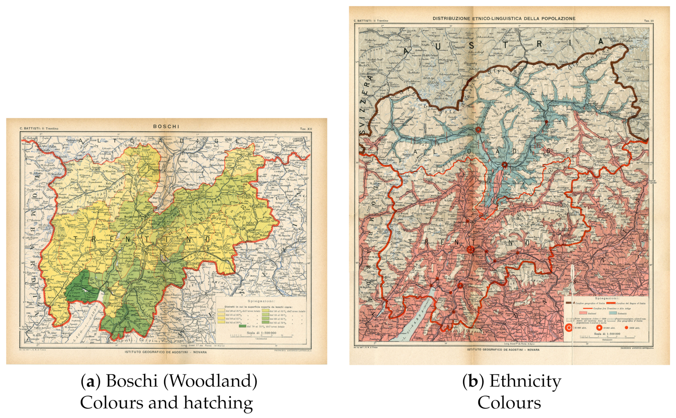
The “Boschi” (Woodland) map (Figure 1a) has been selected both because of its interest for other ongoing research and because it is the more complex in terms of the variety of colours and hatching patterns (Figure 2). For example, the population ethnicity map in the same set (Figure 1b), whose classification is described in [37], has no hatching and is therefore simpler to classify. The “Boschi”map represents the percentage of forest coverage with nine classes from 30% to 75% with 5% steps, with eight service classes (hydrography, roads, borders of the Kingdom of Italy, borders of the Capitanati administrative areas, borders of administrative districts, cities, text, and area outside the region). The latter classes will be filtered in the final map.

2.2. Methods

The procedure to create a digital map describing the different forest density involves four steps: image segmentation, classification, filtering, and geo-referencing. Image classification is carried out using Object-based Image Analysis (OBIA): an analysis of the application of OBIA to the classification of historical maps can be found in [14] and the comparison with a Maximum Likelihood Classification (MLC) approach for similar maps is discussed in [38]. The advantage of the application of OBIA with respect to MLC lies in the more homogeneous results, on the condition that the segments on the image are correctly formed. The application of neural networks could be useful to identify some discrete objects, such as text labels, but it would require the creation of a large training dataset for the recognition of all the interesting features on the map.

The “Boschi” map presents additional challenges with respect to the usual application of OBIA: some areas are identified by a particular hatching pattern and not by a colour, and there are some artefacts due to the JPEG compression and auxiliary elements, such as labels and grid lines, which must be removed.

2.3. Segmentation

The first step in the OBIA method is the creation of segments on the map. Segments correspond to areas representing a single object, whose radiometric and geometric features are then used for its classification. The procedure creating the segments is called segmentation and must be properly calibrated. In fact, if segments do not correspond to objects on the map, their classification will be difficult or even impossible.

In this application, the region-growing algorithm [39] has been used. This algorithm requires two input parameters: a threshold value and a minimum size value.

The threshold parameter, ranging between 0 and 1, defines the value of the (normalized) similarity below which the neighbour pixels are considered part of the same segment. Lowering the threshold value makes the segmentation algorithm more sensitive to radiometric changes. For a threshold value of 0, the segmented maps are identical to the original maps since each pixel is considered a distinct object [40]. A threshold value of 1 creates a single segment for the whole image, since all pixels are considered similar.

The minsize value is the minimum area in a pixel of a single segment [40], and smaller segments are merged. It must be small enough to allow the recognition of small objects but not too small to avoid the division of larger objects into small segments, which can cause problems during the classification step due to the loss of meaning of the geometric features.

Different analytic methods are available for the optimal determination of these parameters. In this application, the Unsupervised Segmentation Parameter Optimization (USPO) [41] has been tested. The performance of the segmentation is evaluated by the intra-object variance weighted by object size (VW) and the space autocorrelation (SA) [42]: VW measures the homogeneity of the segment and SA estimates the difference between neighbouring objects in terms of spectral response. The best segmentation process maximizes both quantities. When VW and SA are normalized, with values between 0 and 1, it is possible to use their sum (between 0 and 2) to choose the optimal threshold and minsize values.

2.4. Texture

Texture has been used to distinguish the different hatching patterns. Texture not only depends on the scale, but several definitions and implementations for the evaluation of the texture are available. Therefore, tests have been carried out by changing filter sizes, evaluation methods, isotropic and anisotropic configuration, different orientations, and different image bands. The best results in distinguishing between different hatching patterns has been provided by using an isotropic correlation with 7 × 7 filter on all the three RGB bands. Higher values on the different bands correspond to distinct hatching patterns (Figure 3a–c). The hatching with a point pattern cannot be identified using the texture parameters above, but it can be detected with a high pass filter with a 5 × 5 window on the red band (Figure 3d).

These four raster maps have been used as additional bands during the classification.

2.5. Classification

Segments classification is carried out with Machine Learning in R through the Grass v.class.mlR module. A supervised classification is performed, and therefore the creation of a training map containing a set of representative training segments of the classes to be recognized is required. Although it is possible to derive the training segments from any vector map containing the same classes, a procedure has been implemented to be able to use training points instead of areas: segments containing the training points are used as training segments and the information about each points class is assigned to the corresponding segment.

The advantage of this approach is that the manual digitization of points rather than areas is considerably faster, while the geometry of the areas is automatically created by the segmentation process. Additionally, this procedure is independent of the configuration of the segments, therefore the same set of training points can be used to classify different segment maps, for example when different combinations of values of the segmentation parameters are tested.

Both geometric and radiometric features have been used as classification parameters for the 7 bands (red, green, blue, correlation on the red band, correlation on the green band, correlation on the blue band, and high pass filter on the red band). The four geometric features of the segments are area, perimeter, compact circle and fractal dimension, while the five statistics for the seven raster maps are mean, stddev, first quartile, median, and third quartile.

The classification has been performed using four different classifiers: Support Vector Machine With a Radial Kernel (SVMradial), Random Forest (RF) and Recursive Partitioning (Rpart), and K-Nearest-Neighbor Classifier (K-NN). The results from the four classifiers have been combined using four different voting systems, which combine the output of each classifier: Simple Majority Vote (SMV), Simple Weighted Vote (SWV), Best Worst Weighted Vote (BWWV), and Quadratic Best Worst Weighted Vote (QBWWV). The first voter (SMV) choose the category indicated by the majority of the classifiers, the second voter (SWV) weights the votes of the classifiers by their predicted accuracy, and the third (BWWV) and fourth (QBWWV) use respectively a linear or quadratic weighting function, after the elimination of the classifiers with the best and the worst predicted accuracy. In the case of four classifiers, the (BWWV) and (QBWWV) voting systems obviously yield the same result.

3. Results

The segmentation, classification, and filtering methods outlined in Section 2.3, Section 2.5 and Section 3.1 have been applied to the map described in Section 2.1.

The application of the segmentation parameters optimization technique described in Section 2.3 to the maps, using the simple sum of the normalized VW and SA as optimization criteria, has given the results in

Table 1. Optimal segmentation parameters values according to Unsupervised Segmentation Parameter Optimization (USPO) on four regions of the image.

Region	Threshold	Minsize	Optimization Criteria
Ala	0.35	10	1.432
Cles	0.35	10	1.790
Riva	0.35	10	1.616
Trento	0.35	10	1.764

. Tests have been carried out on four different parts of the map, each representing a different combination of colours, hatching, and labels text sizes.

While the fact that the same combination of parameters yields optimal results for all the test regions is encouraging, this approach is not workable. This is clearly visible in Figure 4, which shows the segmentation and classification results for the first test area (Ala) of Table 1 for the optimal set of segmentation parameters. This area corresponds to the lower value of the Optimization Criteria in Table 1, and therefore it is expected to be the most problematic. The horizontal green and yellow lines in Figure 4a, which are part of the hatching in one single area are recognized as separate segments (Figure 4b), and thus it would be impossible to classify this area according to its hatching pattern. This effect is clearly visible in the corresponding classified map (Figure 4c)

The reduced effectiveness of the USPO approach when objects with very different sizes are visible on the same map is well known [41]. Therefore, the threshold and minsize combination has been chosen in a two step procedure. The minsize parameter has been set to 10 [pixel] to ensure that the smallest objects on the map, the letters in the labels text, can be recognized. With the minsize fixed to 10, the threshold value has been chosen so that the correct segments are created for all the areas containing hatching, regardless of the pattern and of the colours. Tests have identified the value of 0.25 as optimal in this regard. The final segments map is visible in Figure 5, where the correct identification of the segments, regardless of the hatching, can be appreciated.

The particular of the segments map in Figure 6, at the centre of the map around the city of Trento, shows that there still are some very small areas, usually inside letters, where the information about the hatching pattern is lost and a different segment is created (Figure 6b). These segments are impossible to classify correctly and will be removed during the post-classification filtering phase.

Segments are classified in nine classes corresponding to forest coverage percentage (from 30% to 75% with intervals of 5%) and eight service classes (hydrography, roads, and borders of the Kingdom of Italy, borders of the Capitanati administrative areas, and borders of administrative districts, cities, text, and area outside the region). All the service classes except the last will be filtered. A training set of 298 points, uniformly distributed between the classes, has been manually created and used to classify the map. These points have been used to assign a class to the segment they fall into, creating a map of segments with known classes, which is used as input for the classification procedure, as described in Section 2.5. The result of the classification procedure consists in a vector map with the output of each voting system stored in four columns of the associated table. The corresponding maps are shown in Figure 7.

3.1. Filtering

The map resulting from the classification (Figure 7) must be filtered to obtain area features corresponding to the different forest density classes.

A discussion of the different approaches to text and symbols removal can be found in [14,43], where the approach developed in [14] is used. The procedure comprises two steps: first, the maximum size of objects of the categories to be removed is evaluated, then this size is used for the moving window of a specially crafted low pass filter applied to these categories.

The classification results contain seven service classes (hydrography, roads, boundary Kingdom of Italy, boundaries of the Capitanati administrative units, administrative boundaries of the forest districts, city, and text labels) that must be filtered. The map has been re-classified, merging these eight classes into a single class to be removed.

The minimum, mean, and maximum size of objects to be removed has been evaluated using GRASS’ r.object.thickness add-on module. The size of the low pass filter must be set larger than the $ceil(maximumsize/2)+1$ [14]. The size values for the objects in the class to be removed, in pixels are: minimum 0.000074, mean 2.130567, and maximum 72.504861. Therefore, a filter size of 37 (minimum odd integer ≥ ceil(72/2) + 1) has been used to obtain the maps in Figure 8.

Small segments incorrectly classified are still present, mainly due to the difficulty in identifying the presence of hatching in small spaces within letters on the map, as indicated in Section 2.3. This effect, visible in Figure 6b, inevitably leads to the incorrect classification of these small segments.

To solve this problem, a two step procedure has been used:

• All areas with a size below 1000 pixels have been assigned a new class;
• The procedure for the filtering described above is applied to this new class.

The resulting maps are much cleaner, as shown in Figure 9.

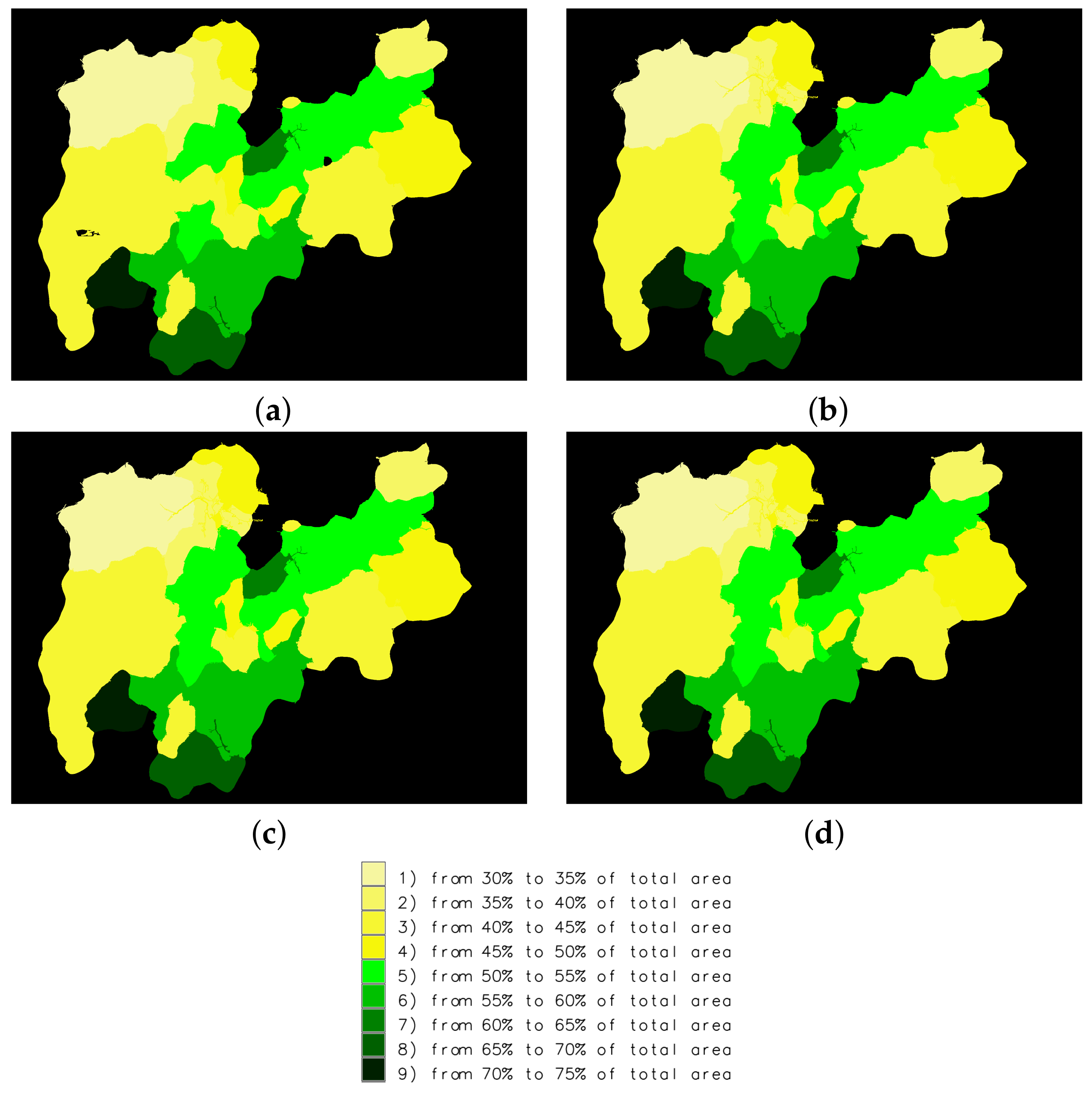
Some artefacts are still visible in the map corresponding to the Simple Majority Vote (SMV) voting system (Figure 9a), while, as expected, the maps for the Best Worst Weighted Vote (BWWV) and Quadratic Best Worst Weighted Vote (QBWWV) voting systems (Figure 9c,d) are identical.

3.2. Georeferentiation

The map must be geo-referenced before it is used in a GIS. This transformation always involves a resampling of the image pixels, therefore it has been performed as the last step of the procedure to avoid the application of the segmentation and classification processes on a resampled image.

The original map is in the Italian pre-Rome 1940 datum, whose definition and transformation parameters are uncertain [44]. For this reason, the map has been geo-referenced in two steps: from pre-Rome 1940 to ETRS89 lat/long (unprojected) (EPSG 4258) using the coordinates of four points of the kilometric grid as reference and a first order polynomial transformation and from ETRS89 lat/long (unprojected) (EPSG 25832) to ETRS89 UTM32N (EPSG 25832) using the standard projection transformation and parameters available through the PROJ.4 library.

The maps have a ground resolution of 54.48 m in the east direction and 79.47 m in the north direction. Assuming a standard graphic error of 0.2 mm on the map, the accuracy at the 1:500,000 scale is of 100 m. Maximum deviations on control points used in step 1 are smaller than one pixel, and are therefore less than 100 m. The additional uncertainty on the map coordinates can therefore be neglected.

3.3. Assessment of the Classification

The digitized maps in Figure 9 have been checked against control maps created by manually digitizing two test areas for each class. The results are shown in

Table 2. Values of Kappa and accuracy (% observed correct) for the classification of the maps with the four voting systems: Simple Majority Vote (SMV), Simple Weighted Vote (SWV), Best Worst Weighted Vote (BWWV), and Quadratic Best Worst Weighted Vote (QBWWV), after filtering.

Voter	Kappa	Accuracy
SMV	0.96	96.77%
SWV	0.97	97.56%
BWWV	0.97	97.57%
QBWWV	0.97	97.57%

, which reports the values of Coehn’s kappa and overall accuracy (% observed correct) for the four voting systems.

The map resulting from the Simple Majority Vote (SMV) has lower values of kappa and accuracy because of some misclassified segments and because the filtering process has not been able to remove all the auxiliary categories, as can be observed in Figure 9a. As predicted, given that only four classifiers have been used, Best Worst Weighted Vote (BWWV) and Quadratic Best Worst Weighted Vote (QBWWV) yield the same map, and therefore the same values for kappa and overall accuracy.

3.4. Forest Density Change

In recent years, many studies have been devoted to assessing the changes in wooded areas extension at local, regional, or national scales, as well as to identify “ancient woodlands” geographies [45,46]. International literature is mainly divided into two different interpretative framework. According to a degradation approach, the relationship between human society and forest in the last centuries is a history of consumption; wooded areas have mostly decreased in extension from XVIII to XIX centuries, and anthropic or natural processes of reforestation are needed to increase biodiversity and to decrease hydrogeological vulnerability of mountains areas [47]. On the other hand, a different approach highlights the positive effects of human practices and rural productions in the management of wooded areas, and claim for the rediscovering and reintroduction of past practices of forest resources use. Ecologists such as Oliver Rackham [34] and Frans Vera [48] discussed the idea of a pristine “natural forest” in all the continents, instead suggesting the presence of a shifting mosaic of open areas, mature trees, and regeneration patches.

The debate is still open, especially because it has important consequences in the development of current policies of environmental heritage management. For this reason, new research and new sources that can allow a better understanding of wooded areas history and their geography in the past are required [33,49].

In particular, the transformations that occurred in the alpine areas during the XIX century in terms of changes in land use and the expansion or decrease of forest coverage have attracted the interest of geographical-historical research, with the aim of identifying the so-called “driving forces” that rule the evolution of territorial and landscape transformations [50]. In this regard, the study of the quantitative variation in the extension of the vegetation cover appears of great interest also because it is closely connected with the abandonment of rural production activities and the decrease of populations in internal communities [51,52], particularly during the decades of the Trentino economic boom.

In fact, in 1919, the territory of present-day Trentino-Alto Adige became part of the Kingdom of Italy as a consequence of the First World War; the restructuring of the production sector caused by the changed geopolitical framework (which also includes a new forestry legislation) was followed by the forced industrialization promoted by the Regime and finally by the economic boom of the 1950s. In this regard, the cartographic source on the percentage of wooded area out of the total produced in the 1910s by Cesare Battisti through the collection of cadastral statistics and forest authority data allows to add a further level of information to the epistemological-cartographic framework on the history of the wooded areas, which can already benefit from sources such as the Habsburg Land Registry (1853–1861) and the Forest Map of the Kingdom of Italy (1936) [4,53].

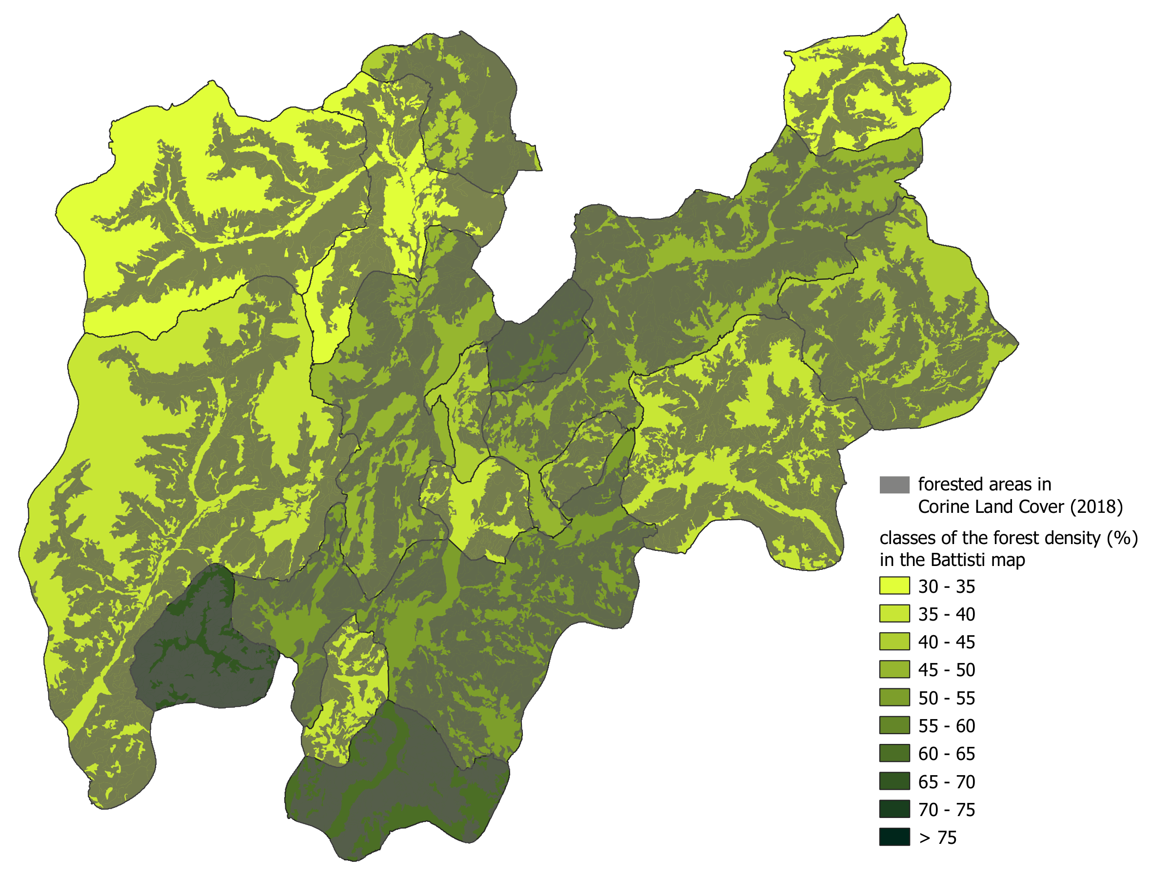
In this case, Battisti’s cartography does not present the topographical location of the forest areas, but their importance in percentage terms in the total area of the Forest Districts into which Trentino was divided. The result of the vectorization operation can therefore be profitably adopted to carry out a comparative analysis of the percentage of wooded areas with the current one, to highlight the changes that have occurred over a century. As a source of information for the current status, the forest cover layer derived from the 2018 Corine Land Cover survey has been used. In particular, the land use and land cover polygons corresponding to the Corine Landcover codes “3.1. Forest” and “3.2.4. Transitional woodland/shrub” [54] have been selected. The polygonal layer with the current extension of the wooded areas was superimposed on the polygonal of the areas with a homogeneous percentage of forest cover resulting from the vectorization of the Battisti map using QGIS, after some small manual corrections, and GRASS GIS (Figure 10).

Through the intersect function, it was possible to merge the two different layers, producing a new polygonal layer with the attributes of the two originals. This operation made it possible to calculate the current percentage of woodland surveyed area in the polygons designed by Cesare Battisti, thus allowing the comparison of the forest state of 2018 with that of the 1910s.

The result is shown in

Table 3. Comparison of forest density according Battisti’s map (1915) density classes and Corine Landcover (2018) “3.1. Forest” and “3.2.4. Transitional woodland/shrub” classes. Area IDs correspond to area labels in Figure 11a.

Area ID	Density Class	Density	Total Area [km${}^2$]	Forest Area [km${}^2$]
	(Battisti)	(Corine)		(Corine)
1	30–35	45.0	708	319
2	35–40	57.1	301	172
3	45–50	75.9	200	152
4	40–45	54.7	1263	691
5	70–75	79.3	181	144
6	55–60	67.2	751	505
7	40–45	54.9	103	57
8	65–70	66.3	271	180
9	50–55	61.0	477	291
10	45–50	37.3	66	25
11	40–45	60.5	110	66
12	60–65	85.6	94	80
13	50–55	67.7	767	519
14	35–40	44.4	206	91
15	45–50	63.8	444	284
16	40–45	65.1	565	368
17	45–50	76.9	55	43

and in Figure 11. The comparative analysis allows to verify how in almost all areas of the province the percentage of wooded areas has increased significantly in the last century. The increase appears generalized and substantially homogeneous, with some areas where it is more pronounced such as in the areas of Fondo, Ledro, Cembra, and Valle dei Mocheni (areas number 3, 5, 12, and 17 in Figure 11), where the current forest coverage exceeds the 75% of the total area. The only exceptions in this trend are represented by the Trento north–Lavis area (area number 10 in the centre of Figure 11), where the urban and industrial expansion of the last decades has been reflected in a strong anthropization of land uses and the decrease of the forest cover, which has fallen below 45% of the total surface, and the southernmost area, where the forest extension is constant. In general, therefore, the processing of the Battisti’s source and the comparison with the current data allows to confirm the hypothesis that sees the exodus of the population towards industrial and service centres and the strong decrease of the agro-forestry-pastoral activities of the last decades as a condition for a progressive re-colonization of meadows and pastures by woody vegetation in Alpine areas [49,51].

4. Conclusions

This study provides an assessment of the application of OBIA procedures for the semi-automatic digitalization of heritage maps containing hatching. The results represent an improvement over the use of Maximum Likelihood Classification (unsupervised, supervised, or supervised contextual) on similar maps [38], and extend the methods described in [14] to maps containing hatching. Values of Coehn’s kappa and overall accuracy in Table 2 demonstrate the viability of the approach. The text and symbols removal technique is effective, as shown in Table 2 and Figure 9.

The use of artificial bands, in particular the texture, is essential for the correct detection of hatching patterns and the correct classification of the areas. Without using texture maps as additional bands, the segmentation procedure identifies each element of the hatching pattern as a separate segment and it is impossible to correctly classify the area.

Some negative aspects still remain: many parameters (for segmentation, texture evaluation, and classification) have to be calibrated and no satisfactory analytical method is currently available. This means that the results depend on the expertise of the operator.

A new procedure is under development for the automatic detection and counting of symbols, to extend the method to maps where the value of an attribute is represented by the number of times a symbol is repeated inside each area. Additionally, the possibility of the automatic extraction of text labels, identifying text string and their position and orientation, is being investigated. This would lead to the creation of an additional vector layer containing toponyms and labels.

All the material and software used in this research, including modules developed ad hoc, is available as Free and Open Source Software in public repositories, making it possible to check the results and easily extend the methods presented in this paper to other datasets.