1. Introduction
Inferring transportation modes is a crucial component of intelligent transportation systems. The transportation mode selected by the traveler is a fundamental behavior characteristic. Inferring transportation mode distributions can help city management agencies understand residents’ behavior [
1] and control the urban transport system [
2,
3,
4]. In addition, transportation mode information plays a vital role in the construction of an activity-based user model [
5] and the provision of task-centered supports [
6]. For example, transportation mode identification helps with customizing mobile services [
7] and with advertising recommendations [
8]. In recent years, an increasing number of cities have begun to deploy Mobility as a Service (MaaS). This new demand-oriented transportation service will change the travel behaviors of urban residents. In order to predict and meet the travel needs of urban residents in a reasonable manner, the basic problem of identifying the transportation mode of residents must be solved.
In the past few decades, the use of GPS devices represented by smartphones has become widespread, and has produced massive amounts of resident data with spatio-temporal information, which offers an excellent opportunity to analyze urban transportation modes at low cost and with high efficiency. However, inferring transportation modes from the raw trajectory is not easy, and still faces several challenges.
To begin with, raw GPS records only contain timestamps and location information, which do not directly reflect trajectory characteristics. Different from image data, using deep learning models to extract features directly and automatically from the raw GPS trajectories is difficult. Therefore, the first problem in transportation mode identification is how to construct an effective representation of the raw trajectories that can also be used by the model. The main method of existing research is to extract a series of motion features. However, in real-life scenarios, the users’ GPS trajectories are influenced by complex geographic information [
9]. Previous studies have demonstrated excellent traffic forecasting capabilities by exploiting the spatial topological relationship in road networks to learn the spatio-temporal dependency of traffic flows [
10,
11]. Moreover, the geographic context supplements valuable information for predictions, and has made a decisive contribution to predictions and forecasts of air quality by using limited sensor data [
12,
13] and mining moving behavior based on trajectory data [
14].
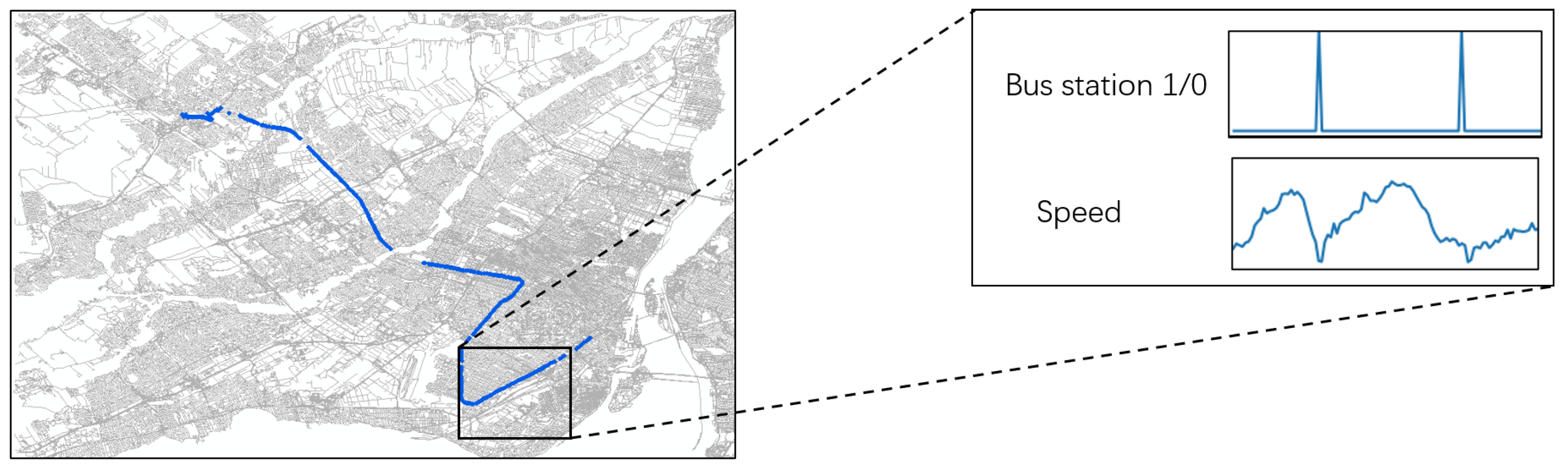
In recent years, studies show that the relationship between GPS readings and geographic information contributes to transportation mode identification. For example, the motion characteristics for the same type of vehicle may vary because they should obey the different velocity limits on the different city roads [
15]. As shown in
Figure 1, we use 1 and 0 to indicate whether there is a bus station within 100 m of the GPS readings. The velocity characteristics of this trajectory are significantly affected as it passes through the bus station. It can be seen that the motion characteristics of the trajectories in the city are affected by the surrounding facilities. It is desirable to construct the representation of the trajectories combined with their own characteristics and the surrounding geographical context [
9,
16,
17]. Therefore, we encode geographic information (e.g., the level of the road network, the distribution of public stations) and fuse it with the motion features of each GPS reading of the trajectories to build the trajectory embedding.
Second, the raw GPS trajectories collected from GPS-enabled smart devices do not directly contain the exact transportation mode labels. Therefore, to construct the sample for training the supervised learning model, users or researchers often assign transportation mode labels to the trajectories manually, which makes the studies based on the supervised learning model face the same limitations as traditional travel survey research. Unlike images and natural language texts, the trajectory composed of GPS readings is difficult for researchers to understand, making annotating labels a very time-consuming task. Furthermore, it is often costly for a large number of users to annotate their trajectories. For example, as introduced by Stopher and Greaves [
18], it costs USD 750 to collect a week’s worth of user data. Compared with the high-cost label annotation, a large number of unlabeled GPS trajectories are easy to obtain. Therefore, it is necessary to design a model that can help us automatically extract information that is helpful for transportation mode identification from the easily obtained unlabeled data.
Based on previous studies [
15,
17,
18], there are two research questions for transportation mode identification on GPS trajectories, i.e.,: 1. How can heterogenous features be integrated, such as motion features and geographic information, to represent a trajectory? 2. How can a semi-supervised transportation mode identification model be built with only a small amount of labeled trajectories and a large number of unlabeled trajectories?
In order to solve the above problems, we propose a novel transportation mode identification framework, named GeoSDVA, in which we first generate the embedding of trajectory with the combination of the motion features and geographic information of each GPS reading of a raw trajectory, and then construct a semi-supervised transportation mode identification model based on a Dirichlet variational autoencoder. Accordingly, the main contributions of the study are summarized as follows:
We propose a new sample design method to fuse the heterogeneous features together, including the geographic information and motion features from the raw trajectories. This method integrates the motion features and geographic contexts to which the GPS trajectory is related, including the bus stations, road intersections, and the road network level, to form an embedded representation of the raw trajectory;
We construct a semi-supervised Dirichlet variational autoencoder (DirVAE) based the transportation mode identification model, named GeoSDVA, which consists of three modules: an encoding module to encode trajectories into latent vectors, a classifier module with multi-scale convolution to extract multi-scale features and predict the transportation modes of trajectories, and a decoding module that reconstructs the input trajectories;
We conduct extensive experiments on three real-world datasets, namely, Geolife v1.3, MTL Trajet 2017, and MTL Trajet 2016. The experimental results show that GeoSDVA outperforms other state-of-the-art frameworks. Furthermore, we evaluate the identification metrics of GeoSDVA under different amounts of labeled trajectories. The evaluation results show that GeoSDVA is practical for identifying the transportation mode of trajectories, especially when a small number of labeled trajectories are included in the training datasets.
4. Experiment Results
In this section, we explain and discuss the results of GeoSDVA through a series of experiments. All experiments are performed on the same PC with a Core i7 3.20 GHz processor and 32.0 GB memory. All models and experiments are implemented via TensorFlow v1.8 and Scikit-learn.
4.1. Gps Data
In this paper, three real-life datasets, Geolife V1.3, MTL Trajet 2017, and MTL Trajet 2016, are used to evaluate the proposed approach. An overiew of these three datasets is shown in
Table 2.
The Geolife v1.3 dataset collected five years’ worth of GPS data from 182 users between April 2007 and August 2012. Among these users, 73 of them have marked their transportation modes. The transportation mode labels of trajectories in the Geolife dataset mainly include walk, bike, bus, car, taxi, train, subway, airplane, boat, run, etc.
The MTL Trajet 2017 dataset collected the GPS data of 4425 users from 18 September to 15 October 2017. In the MTL Trajet 2017 dataset, user-labeled transportation modes include public transportation, walk, car/motorcycle, bike, car sharing, taxi, etc.
The MTL Trajet 2016 dataset collected GPS data from September to November 2016. In this dataset, user-labeled transportation modes include public transportation, walk, automobile, bike, etc.
There are three main reasons for why we use these datasets to explore the performance of the GeoSDVA model. First, most of the trajectories in these datasets are collected in an urban environment, so we can obtain the corresponding GIS data through open data sources. Second, there are more than three transportation modes in these datasets, which enables us to verify the transportation mode identification performance of GeoSDVA. Third, and last, the datasets are composed of some labeled and some unlabeled trajectories, which enables us to explore the semi-supervised learning ability of GeoSDVA.
In order to ensure that the GPS trajectories can be associated with GIS data, we filtered the data according to geographical areas. For the Geolife dataset, we selected the GPS readings in Beijing (116.15° E, 39.75° N to 116.6° E, 40.1° N), accounting for about 70% of the total dataset. For the MTL Trajet 2017 and the MTL Trajet 2016 datasets, we selected the GPS readings in Montreal (73.942° W, 45.415° N to 73.479° W, 45.701° N), accounting for about 90% of each dataset.
We selected only ground transportation modes for the experiment. In the Geolife dataset, trajectories labeled as taxi, car, bus, walk, and bike are selective objects, with car and taxi falling into one category and labeled as “car” in particular. Finally, the experimental dataset covers four transportation modes: bike, public transit (bus), car, and walk. The trajectories with other labels or without labels are considered unlabeled trajectories. In the MTL Trajet 2017 dataset, we selected the trajectories labeled as public transit, taxi, car-sharing, car/motorcycle, bicycle, and walking for the experiment. The data labeled as car-sharing, taxi, and car/motorcycle are combined as “car”. Ultimately, the dataset contains four labels: walk, public transit, car, and bike. The trajectories with multiple labels, with other labels, and without labels are regarded as unlabeled trajectories. In the MTL Trajet 2016 dataset, we select the trajectories labeled as walk, bike, public transit, and automobile. The data labeled as automobile are relabeled as “car”. Finally, the dataset contains walk, bike, public transit, and bike. The distribution of various label trajectories in each dataset is shown in
Table 2.
4.2. GIS Data
The GIS data we use is mainly come from the road network data of OSMNX [
42]. The road networks of Beijing and Montreal are shown in
Figure 4. Road network data consists of road network nodes and road network edges. Taking the Beijing road network data as an example,
Table 3 shows partial data of the road network edge, and
Table 4 shows partial data of the road network node. For the road network edges, we determine the level of the road network based on the value of the highway attribute, which mainly includes “motorway”, “trunk”, “primary”, “secondary”, “tertiary”, “unclassified”, and “residential”. For the road network nodes, we filter the nodes with the highway attribute values of “crossing”, “traffic_signals”, and “motorway_junction”. For the bus station data, we use a public data source to extract their coordinates. The data of bus stations in Beijing comes from public SHP files; the data of bus stations in Montreal comes from Google Transit API.
4.3. Experiment Setup
In the experiment, several typical evaluation metrics, such as accuracy, precision, recall, and macro F1-score, are employed to evaluate the performance of the proposed model. The calculation methods in this paper are shown in Equations (
17)–(
21). In the confusion matrix of the multi-class identification, when these evaluation metrics are calculated for each category, the samples that belong to this category are considered positive. The samples that do not belong to this category are negative. Accuracy is used to evaluate the overall identification of the model in the test set. Since the transportation mode in the datasets are unbalanced, the macro F1-score is used to evaluate the overall performance of the model in identifying each transportation mode in the test set.
In all experiments, L is set to 100. If the number of GPS readings in a segment is less than 100, we use linear interpolation for it. At the beginning of model training, the loss of encoder is much greater than the loss of classifier, which will lead to the optimizer ignoring the loss of classifier. In order to alleviate this problem, we set in the loss function to 0.1 to weigh the relative importance between classifier loss and encoder loss.
In the following subsection, we evaluated the performance of GeoSDVA on semi-supervised transportation mode identification. Firstly, the proposed GeoSDVA was compared with other baseline methods by the experiment to explore GeoSDVA’s ability to use information from unlabeled trajectories under the guidance of different numbers of labeled trajectories obtained by adjusting their ratios. Secondly, we analyzed how the knowledge learned by DirVAE from unlabeled trajectories helped the task of transportation mode identification. Finally, the transportation mode of unlabeled trajectories in specific areas was identified using the trained GeoSDVA, and its results were analyzed.
4.4. Benchmarks
To illustrate the advantages of GeoSDVA, we compare the proposed model with several baseline methods, listed below:
DT: This method, developed by Zheng et al. [
19], extracts some statistical features from the GPS trajectory segment and identifies the transportation mode through a C4.5 decision tree;
RF: This method, developed by Xiao et al. [
31], utilizes tree-based ensemble models, such as random forests, to infer the transportation modes;
SVM: This method, developed by Bolbol et al. [
43], uses segment-level statistical features and an SVM to identify transportation modes;
DNN: This method, developed by Endo et al. [
23], uses a dense network to extract features from the images composed of meshed trajectories and to identify transportation modes;
CNN-GAN: This method, developed by Li et al. [
34], uses generative adversarial networks to expand the labeled trajectory dataset, and adopts the enhanced dataset to train a six-layer CNN network for transportation mode identification;
SECA: This model, developed by Dabiri et al. [
44], follows the autoencoder framework for semi-supervised learning and uses a six-layer CNN network as both an encoder and a classifier to share weight between the labeled and unlabeled trajectories.
Pseudo-label: This model, developed by Dabiri et al. [
44], uses a self-training strategy for semi-supervised learning;
Two-step: This model, developed by Dabiri et al. [
44], features a two-step training model which first trains the encoder–decoder network and then trains the classifier based on the encoder’s latent vector.
It should be noted that the sample forms required by these methods are different. For experimental fairness, all samples are generated from the same dataset composed of raw GPS trajectory segments. During the experiment, labeled trajectories are divided into train datasets and test datasets, according to the ratio of 8:2, and all unlabeled trajectories participate in the training. By changing the number of labeled trajectories, we randomly sample the training dataset according to the label proportion. Meanwhile, the unlabeled dataset remains unchanged.
4.5. Identification Performance
Firstly, we validate the advantage of our proposed GeoSDVA mode over its counterparts. We build the GeoSDVA and other baseline methods separately with varying amounts of labeled trajectories, and then evaluate them on the same test dataset. The evaluted results between GeoSDVA and other baseline methods on three real datasets are listed in
Table 5,
Table 6 and
Table 7, with the best performances shown in bold. The percentage in the first row of the tables represents the sampling rate of the labeled training dataset. For example, 10% means that only 10% of the labeled trajectories participated in the training.
According to
Table 5,
Table 6 and
Table 7, GeoSDVA performs better in identifying transportation modes than the baseline method under any sampling rate of labeled trajectories. The experiments SVM, DT, and DNN, which use two datasets and are based on supervised learning, generally show disadvantages compared with other methods. When the sampling rate of labeled data is low, compared with other supervised learning methods, RF shows some advantages. However, its identifying performance is not good enough when the sampling rate of labeled data is significant. Moreover, it is worth noting that the two-step model performs poorly on both datasets, especially on Geolife, as is seen from
Table 5. In the two-step model, the classifier does not participate in the first training step, which may lead to the encoder’s failure to learn the information that is helpful for transportation mode identification. Compared with the SECA, pseudo-label, and CNN-GAN, the macro F1-score of GeoSDVA improves from 4% to 7% in the Geolife dataset, from 0.4% to 3% in the MTL Trajet 2017 dataset, and by over 0.8% in the MTL Trajet 2016 dataset when the sampling rate is 10%. SECA uses an autoencoder and classifiers with shared weights for semi-supervised learning. Due to the lack of constraints on the latent vector learned by the autoencoder, SECA cannot effectively use the unlabeled trajectory when there is less labeled data. The pseudo-label method labels the unlabeled trajectories in the training process continuously, but the pseudo-label of the unlabeled trajectories may be wrong. The CNN-GAN method uses labeled trajectories to expand the dataset through a GAN network, rather than using unlabeled trajectories for learning. When all labeled data are used to train the model, GeoSDVA can still achieve the best performance. Compared with other methods, its macro F1-score improves by about 2% on the Geolife dataset, from 0.6% to 1.6% on the MTL Trajet 2017 dataset, and by at least 2% on the MTL Trajet 2016 dataset. This is because GeoSDVA uses GIS features that are not used by other models, which makes it easier to distinguish between transportation modes.
Overall, there are two main reasons why GeoSDVA has advantages over the baseline model. First, GeoSDVA combines the geographic information around the trajectories, which makes it easier to distinguish between different transportation modes, resulting in a higher macro F1-score. Second, compared with the semi-supervised models based on deep learning, such as the SECA, two-step, and CNN-GAN methods, the semi-DirVAE in GeoSDVA can better extract the features from the unlabeled trajectories, enabling a better performance when there are few label trajectories. We will analyze the role of these two factors in the following subsections.
4.6. Advantage of Semi-Supervised DirVAE
In this subsection, we analyze the advantage of the semi-supervised DirVAE in the model. Firstly, with varying amounts of labeled trajectories, we separately build the GeoSDVA and the supervised-GeoSDVA, which is a variant model that only retains the classifier module. We test the two models on the same test dataset and analyze the impact of the semi-supervised DirVAE on transportation mode identification.
Table 8 show the comparison between GeoSDVA and supervised-GeoSDVA. The comparison results indicate that GeoSDVA performs significantly better than supervised-GeoSDVA, especially in the case of fewer labeled trajectory datasets. Obviously, it can been seen the macro F1-score of GeoSDVA improves from 7% to 8% when 10% of the labeled trajectories are in training. While all labeled trajectories are involved in training, the macro F1-score of GeoSDVA is about 2–6% higher than that of supervised-GeoSDVA. The experiment results show that no matter how many labeled trajectories participate in the training, the transportation mode identification performance of the model is improved when DirVAE is added. When the proportion of labeled trajectories is relatively low, the improvement brought by DirVAE is very obvious, especially in terms of macro F1-score, taking the identification results on the MTL Trajet 2016 dataset when the label data proportion is 25% as an example.
Figure 5a,b shows the confusion matrices of GeoSDVA and supervised-GeoSDVA, respectively. Due to the small amount of labeled trajectories, the supervised-GeoSDVA identifies a large number of trajectories as car and public transit incorrectly. As a comparison, the identification result of GeoSDVA does not have this problem. This proves that the addition of DirVAE can make the model obtain better identification results when there are fewer labeled trajectories.
To further analyze how the semi-supervised DirVAE uses unlabeled data to help with transportation mode identification, we extract the latent vector of the DirVAE encoder module from the pre-trained GeoSDVA. For three datasets, a random sample of 20,000 trajectory segments is taken from both labeled and unlabeled trajectory datasets, respectively. Then, these trajectories are input into the pre-trained GeoSDVA to obtain their latent vectors.
Figure 6 shows the distribution of the latent vectors after the T-SNE dimensionality reduction.
Overall, the latent vectors of different transportation mode trajectories extracted by DirVAE have clear boundaries. From the visualization of the latent vector of Geolife, it is found that the latent vectors of the car (green scatters) and public transit (pink scatters) labels have clear boundaries, but the latent vectors of the bike (blue scatters) and walk (yellow scatters) labels are intertwined in some spaces. This is because some walk and bike trajectories in the Geolife dataset are in a similar geographical environment and have similar motion features. Moreover, a clear boundary between the walk (blue scatters) label and other trajectories appears on the visualization of the latent vector of the MTL Trajet 2017 dataset. By comparison, the boundary between the latent vectors of the public transit (pink scatters), bike (blue scatters), and car (green scatters) labels is not very obvious. On the MTL Trajet 2016 dataset, we also observed that cars (green scatters) and public transit (pink scatters) are intertwined. There are two reasons for this result. In the MTL Trajet 2017 dataset, car trajectories are much more common than other transportation mode trajectories. In the MTL Trajet 2016 dataset, car trajectories account for more than 60% of the total. Second, some trajectories labeled as public transit in the MTL Trajet 2017 and MTL Trajet 2016 datasets do not stop near bus stations periodically during movement. These trajectories may not be recorded under bus or railway mode, which makes it difficult to distinguish these trajectories from car trajectories.
4.7. Influence of Geographic Information
In this subsection, we analyze the role of geographic information in transportation mode identification. We speculate that, in urban areas, the geographic information around the trajectory is helpful for distinguishing transportation modes. We delete three features related to geographic information in trajectory embedding, and then train the GeoSDVA model on two datasets, respectively. In
Table 9, we use “Motion+GIS” and “Motion” to distinguish between models with different features.
According to the experimental results, on the Geolife dataset, the F1-scores of public transit, car, and walk have been improved with the supplementary geographic information. Among them, the F1-score of the car trajectories increased most significantly, to 6%. At the same time, the F1-score of the bike trajectories decreased by about 0.5%. Comparatively, on the MTL Trajet 2017 dataset, the supplement of geographic information has improved the F1-scores of all transportation modes, as is demonstrated in the above table, with the increase of public transit, bike, car, and walk, respectively, by 0.6%, 0.4%, 0.1%, and 1%. On the MTL Trajet 2016 dataset, the supplement of geographic information has improved the F1-scores of public transit, bike, car, and walk, respectively, by 6%, 0.6%, 1.2%, and 4.8%. From a macro point of view, the identification performance of GeoSDVA has been improved with the supplement of geographic information on three datasets.
We visualized the confusion matrices of three datasets with different features, as shown in
Figure 7,
Figure 8 and
Figure 9. On the Geolife dataset, the typical misclassification occurs between bike and walk, as well as between public transit and car. The addition of GIS features improves the identification accuracy of public transit, bike, and car, but reduces the identification accuracy of walk. According to the confusion matrix, the misclassification of public transit as car is reduced by 0.8%, and that of car as public transit is reduced by about 1.4%. Similarly, the misclassification of bike as walk is reduced by about 1.2%, while the misclassification of walk as bike is improved by 0.6%. The reason for the reduction may be that walk and bike have similar GIS features. On the MTL Trajet 2017 dataset, it is difficult to correctly identify public transit trajectories, which will be incorrectly identified as car and walk. The addition of GIS features improves the identification accuracy of all transportation modes. However, the addition of GIS features cannot effectively distinguish public transit from car. The proportion of misclassifications of public transit as car has hardly changed. The improvement of public transit is mainly due to fewer misclassifications as walk and bike. The public transit trajectory in this dataset may include other modes, such as ferry cars, that do not stop at bus stations, which makes it difficult to distinguish between public transit and car. On the MTL Trajet 2016 dataset, the results observed are similar to those on the MTL Trajet 2017 dataset. GIS features improve the identification accuracy of all transportation modes. The addition of GIS features does not increase the proportion of public transit trajectories misclassified as car trajectories, but significantly reduces the proportion of public transit trajectories misclassified as walk trajectories. Moreover, the proportion of bike misidentified as car is reduced by 2%, and the propotation of car misidentified as public transit is reduced by 2.3%; the walk identification is not improved significantly. In general, the addition of GIS features improves the accuracy of transportation identification on each dataset.
4.8. Case Study
In this subsection, we use GeoSDVA to analyze the distribution of transportation modes in a specific area of Beijing, located between (116.300831° E, 39.971985° N) and (116.333889° E, 40.026152° N), as shown in
Figure 10a. In this area, there is a university campus, around which there are some roads. In order to better explain our results, we visualized the road level and bus stations in this area, as shown in
Figure 10b. It can be seen that the university campus is surrounded by “Primary” and “Secondary” level roads, while the road level inside the university campus is “Unclassified” and “Residential”. In addition, the cyan diamond symbols represent the locations of bus stations. In this area, bus stations are mainly distrbuted on high-grade roads, such as “Primary” and “Secondary” level roads. Obviously, there are no bus stations inside the university campus. We have selected all trajectories located in this area that were not marked by the user from the Geolife dataset, and utilized the pre-trained GeoSDVA model to identify the transportation modes of these trajectories. Since the GeoSDVA model requires an input with fixed length, we use the sliding window and maximum vote to determine the transportation mode of a trajectory.
Figure 11 shows the four transportation mode trajectories identified by GeoSDVA in this area, respectively. The identification results indicate that a large number of walk and bike trajectories exist inside the university campus, while public transit and car trajectories rarely appear there. Inside the university campus, people tend to walk and use bikes, while the use of cars in this area may be limited. For a better explanation, we provide statistics for the proportion of various transportation modes inside and outside the university campus, as shown in
Figure 12. In this area, about 14.3% of the trajectories are walking trajectories and 42.8% are bike trajectories inside the university campus. In contrast, only 2% of the trajectories found inside the univeristy campus are public transit ones, and 3% of them are car trajectories.In addition, we also found some other phenomena. In the northeast section of the area, there is a “Motorway” level road. Walk and bike trajectories are not identified on this road, because these two modes are not allowed to use it. We identified fewer public transit trajectories than car trajectories inside the university campus. This is because there is no bus station inside the university campus, so the bus station has become a strong support to distinguish between the trajectories of cars and public transit in this area. Moreover, we also observed that, compared with the car trajectories, the public transit trajectory appears on roads with a higher road level, which is also determined by the location of bus stations. In general, the identification results of GeoSDVA are consistent with common sense in reality, and its results have reference value.
5. Discussion and Conclusions
This paper proposes a novel semi-supervised model named GeoSDVA to identify residents’ transportation modes. First, the input of GeoSDVA is designed for GPS readings that combine motion features with geographic information. Second, a semi-supervised model based on DirVAE is built to learn features that are helpful for transportation mode identification from unlabeled trajectories. Then, with the evaluation of GeoSDVA on two real GPS trajectory datasets, it is proved that GeoSDVA has the ability of semi-supervised learning when only a few trajectories are labeled, and its performance in transportation mode identification is better than the baseline methods. After that, we analyze how the DirVAE module obtains helpful information from unlabeled trajectories for transportation mode identification. Moreover, we analyze the impact of geographic information on the identification of specific transportation modes. Finally, we use a pre-trained GeoSDVA to label and analyze the unlabeled trajectories in an area, which shows that the identified results have practical significance.
GeoSDVA can be applied to practical decision making by urban management departments and transport companies in view of the following advantages. First, a large number of unlabeled GPS trajectories is easy to collect, while GeoSDVA only needs a few expensive labeled trajectories in the training, which brings a cost advantage. Second, low-carbon travel has now become a hotspot in transportation research areas. There are significant differences in the carbon emissions of different transportation modes. GeoSDVA can be used to identify the carbon emissions of individual travelers, so as to help the government formulate relevant policies to encourage green travel. Third, the transportation mode identification of GPS trajectories in the city by GeoSDVA can help formulate other urban planning schemes. For example, clustered car trajectories in a city can help find frequent paths, so as to set up appropriate public transit routes to meet residents’ travel needs and reduce environmental pollution.
In addition, GeoSDVA has the following advantages over existing transportation mode identification models. Compared with the model that only uses motion features for transportation mode identification, GeoSDVA considers the affect of GIS information on trajectory, and uses deep networks to extract relevant features. Compared with the transportation mode based on traditional machine learning, the GeoSDVA model does not need to design statistical features manually, and can automatically extract features from the raw trajectories. Compared with the transportation identification model based on supervised learning, GeoSDVA can use the unlabeled trajectories to learn, and can use a small number of labeled trajectories for accurate transportation mode identification, which solves the problem of the high cost associated with labeling trajectories. Compared with the semi-supervised transportation identification mode based on an autoencoder, GeoSDVA utilizes a variational encoder structure to build a more constrained latent space and improve the semi-supervised learning ability.
In the future, we will improve and enhance our work from the following three points. Firstly, there may be some transportation modes in the unlabeled dataset that do not appear in the labeled dataset. The trajectories of these unknown transportation modes may bring noise to the semi-supervised learning model. Secondly, privacy protection in location-based services has increasingly become a research hotspot. Transportation mode identification in a privacy-protection scenario is a problem worth studying. Finally, it is very attractive to introduce more GIS features for transportation mode identification. GIS features such as urban land types may be helpful to distinguish between trajectories.


