Abstract
The rapid development of the Chinese economy has stimulated consumer demand and brought huge opportunities for the retail industry. Previous studies have emphasized the importance of estimating regional consumption potentiality. However, the determinants of retail sales are yet to be systematically studied, especially at the micro level. As a result, the realization of sustainable development goals in the retail industry is restricted. In this paper, we studied the determinants of retail sales from two aspects—location-based socioeconomic factors and spatial competition between shops. Using 12,500 retail shops as our sample and by adopting a grid-division strategy, we found that regional retail sales can be positively impacted by nearby population, road length, and most non-commercial points of interest (POIs). By contrast, the number of other commercial facilities, such as catering facilities and shopping malls, and the area of geographic barriers often caused negative impacts on retail sales. As to the competition effects, we found that the isolation and decentralization of shops in one area have a marginally positive effect on sales performance within a threshold distance of 226.19 m for a central grid and a threshold distance of 514.85 m for surrounding grids, respectively. This study explores the determinants of micro-level retail sales and provides decision makers with practical and realistic approaches for generating better site selection and marketing strategies, thus realizing the sustainable development goals of the retail industry.
1. Introduction
With the development of the Chinese economy, the social consumption of consumer goods shows a dramatically increasing trend [1,2]. According to the China Economic Annual Report of 2021 published by the National Bureau of Statistics on 17 January 2022 [3], the total sales of consumer goods in the year 2021 reached CNY 44.1 trillion, showing a 12.5% increase compared with the year 2020 and contributing 65.4% to the total economic growth. The scenario offers huge opportunities for the recovery and development of the retail industry and stimulates the establishment of new retail shops, whose site selection and marketing strategies must be more carefully planned after the experience of the mass shutdown period during 2020 [4,5,6]. Therefore, studying the determinants of retail shop sales from a new perspective—the geographical micro level—can be beneficial for the retail industry in adapting its marketing strategies during the post-epidemic period.
Previous studies have documented the effects of macro-scale determinants on retail sales. Macro-scale determinants are mostly socioeconomic statistic metrics, such as gross domestic product (GDP) and population, which are derived from provincial- or national-scale statistical yearbooks. On the basis of statistical data from the retail industry in Ghana, Rowena [7] pointed out that three major independent variables, namely, population size, per capita income, and income elasticity of demand, are positively correlated with total consumption demand. Using common statistical data, Joacim [8] found that the rise in environmental awareness also plays a key role in retail sales by affecting the attitudes of consumers toward excessive consumption. This finding was consistent with that of Plavini [9]. Using census data in the US, Jorgensen found that nearly 22% of the American population will be age 60 and over by 2030 and pointed out that the ratio of the senior population causes different retail trends among states [10]. By observing the sales performance of stores in the UK during the recession in the 1990s, Mavis found that retail sales volume was positively correlated with economic prosperity, and that food stores would suffer more large-scale impacts from the economic fluctuation than non-food stores [11]. The findings obtained through these statistical data can reveal fundamental rules of economic development, which can be useful in predicting the national and provincial consumption potentiality in the next few years [12,13]. However, the application for the findings in microscale studies presents limitations: (1) The statistical data lack information that describes the nearby urban configuration of retail shops, which plays a key role in impacting their sales. The large-scale statistical data pose difficulty for a highly accurate estimation of business potential at smaller scales. (2) The statistical data cannot reflect the geographic relationship and competition between retail shops, which is one of the key factors impacting retail sales.
The micro-scale determinants of consumption potentiality need to be explored, and the geographic factors need to be considered, to provide practical guidance for the retail industry. Although previous studies have pointed out that retail sales are geographically correlated with nearby socioeconomic factors, the mechanism is unclear [14,15]. Exploring the location-based socioeconomic determinants of retail consumption is an urgent matter to provide guidance for governments worldwide to formulate consumption stimulus measures and to help their retailers achieve quick recovery during the post-pandemic era.
Recent studies have realized the importance of micro-level socioeconomic factors and spatial proximity between retail shops and have proposed several models to describe the potential interaction between these factors and regional consumption. Martin [16] proposed the spatial interaction model to describe the consumer appeal of a business district, which was thought to be positively correlated with population size around the district, but negatively correlated with the distance between consumers and the district. On this basis, Convers [17] proposed the breaking-point model to determine the threshold value of distance for the retail attraction between two commercial centers. Besides demographic data, a variety of datasets were adopted for measuring the micro-level attraction of retail facilities. Using Sina Weibo check-in data—a type of location-based social media data—Jiang [18] and Wang [19] proposed a retail competition model to quantitatively measure the competitiveness of each shop by considering the distance and number of check-in records located in nearby regions. On the basis of transportation data, Cohen and Applebaum [20] proved that retail sales can be influenced by car driving time, as well as store area. Using the Visible Infrared Imaging Radiometer Suite nighttime light data, Wang [21] proposed a human-activity model to describe population mobility in different commercial regions and then predicted consumption potentiality by conducting geographically weighted regression. However, the above attempts were mainly conducted through black-box methods, which means the economic relationship between these geographic factors and retail sales has yet been systematically proven.
The determinants of local consumption at the micro scale have been an unsolved but urgent issue in both marketing and geographical science. Hence, this study aims to explore the relationship between a variety of location-based factors, including socioeconomic factors and spatial proximity factors, and regional consumption, with a research object to provide universal guidance for the retail industry. To achieve this goal, we designed a novel experiment using actual sales data and locations of retail shops in Qiannan, China. First, the socioeconomic indexes, including POIs, population data, and road networks, along with a total of 12,500 retail sales data, were extracted and formed into a grid scale by using a grid-division processing strategy. Second, we designed a competition model and calculated two location-based competition indexes, including number-based competition index and distance-based competition index, according to the spatial proximity between shops. Third, all the socioeconomic variables and spatial competition metrics were included in an ordinary least squares (OLS) regression model. The results showed that regional retail sales can be positively impacted by nearby population, road length, and most non-commercial POIs. We also found that the isolation and decentralization of shops in one area has a marginally positive effect on sales performance within a threshold distance of 226.19 m for a central grid and a threshold distance of 514.85 m for surrounding grids, respectively.
The contributions of this work are as follows. In the theoretical aspect, first, we proposed a comprehensive framework to systematically study the determinants of retail sales at the micro level from two aspects—location-based socioeconomic factors and spatial competition between shops—which might expend the previous macro level research perspective. Second, we proposed new approaches to measure spatial competition between shops based on the ratio and distance-based distributions of shops, which are able to better reflect the competitive ability in each grid when compared to considering the number of retail shops; therefore, the methodology proposed can be utilized by future researchers. Third, we found that although the spatial decentralization of the shops’ location may contribute to regional sales, this does not mean that the farther away the shops are, the better. The distances of the shops in the area and the surrounding areas of the shops have inverted U-shaped effects on regional sales, and we obtained the thresholds of the positive effects. In the practical aspect, the methodology and empirical results of the location effect presented can be instructive for marketing practitioners and urban planners to make better site selection decisions by taking advantage of spatial socioeconomic and shop data to realize the sustainable economic benefits of offline consumption industry in smart city construction.
The remainder of this paper is organized as follows: Section 2 describes the study area and dataset used in this study. Section 3 and Section 4 show the methods and experimental results, respectively. Section 5 discusses the robustness check of our results and the limitations of the current work. Section 6 concludes the paper.
2. Materials
2.1. Study Area
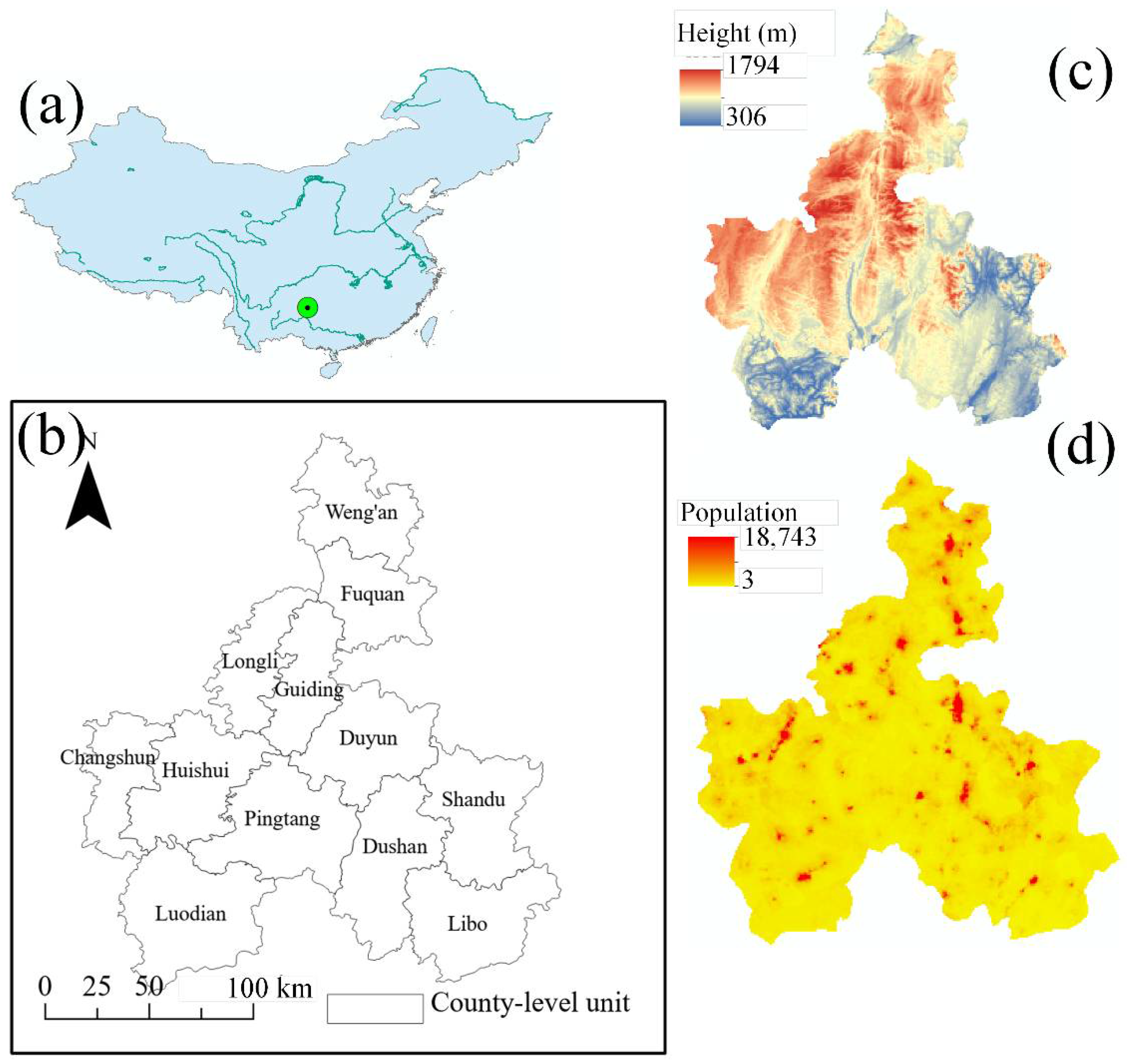
Qiannan Buyei and Miao Autonomous Prefecture (Qiannan), located in the south central area of Guizhou Province in China and near the province’s capital city Guiyang (Figure 1a), is set as the study area. Qiannan belongs to the slope zone from Guizhou Plateau to Guangxi Hills; hence, its terrain is higher in the west and lower in the east, with the maximum height difference reaching 1719 m (Figure 1c). The mean elevation of Qiannan is 997 m, which is lower than the province’s average elevation of 1107 m [22]. The low-lying terrain, along with its subtropical monsoon climate, causes the complex and varied land surface that is characterized by peak forests, peak clusters, trough valleys, depressions, and water holes. Qiannan shows a typical subtropical humid monsoon climate, with an annual average temperature ranging from −19.6 °C to 13.6 °C and the annual precipitation reaching 1200 mm. These characteristics make Qiannan one of the areas with the highest precipitation. With a total area of 26,200 km2, Qiannan includes 12 county-level administrative units (two county-level cities, nine counties, and one autonomous county), as shown in Figure 1b. According to the seventh census of China, Qiannan has approximately 3.49 million long-term residents as of November 2021, and the ethnic minority population accounts for about 59% of the total population (Figure 1d).
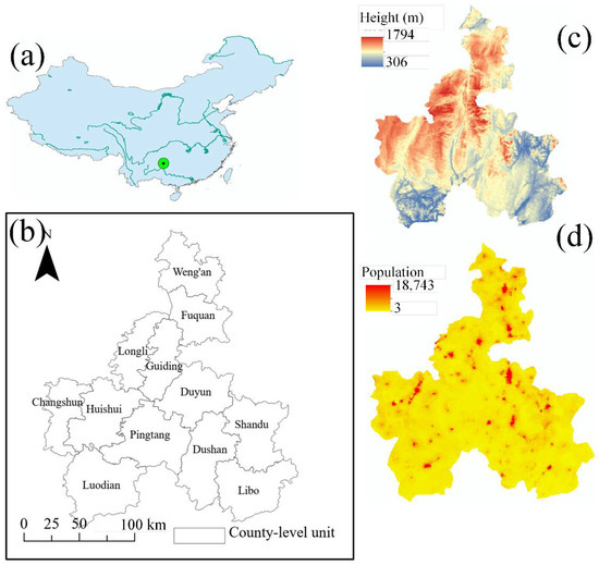
Figure 1.
(a) Location of Qiannan in China. (b) Administrative division of Qiannan. (c) Topography of Qiannan. (d) Population distribution of Qiannan.
The special geographical location and culture largely influence the economy structure of Qiannan, which is relies heavily on its primary industry. According to the statistical data, the share of primary industry in Qiannan reached 15.97% in 2020, which was far larger than the average level of the whole country (7.7%). Benefitting from the “One Belt and One Road” program in China, the social economy of Qiannan has undergone prominent development, with the total GDP reaching USD 23.35 billion in 2019 and a yearly growth of 7.9% [23]. However, its per capital GDP (USD 7300) is just 64% of the average level of the whole country, and it even shows a decreasing trend in 2020, due to its population growth rate being larger than its GDP growth. That makes Qiannan different from the environment of large developed cities and enlarges the significance of studying its regional retail sales.
According to the National Bureau of Statistics, the total retail sales of consumer goods in 2019 reached USD 4.56 billion, up to 3.3% over the previous year. The retail sales of urban areas reached USD 4.30 billion, with an annual increase of 3.2%; the retail sales of rural areas reached USD 0.26 billion, with an annual increase of 4.4%. The consumption pattern shows that the income of the catering service was 0.87 USD billion, with an annual increase of 11.5%, and the income of consumer goods was USD 36.7 billion, with an annual increase of 1.5%. The rapidly developing economy has attracted many foreign investments. In 2019, the total foreign investments reached USD 9.4 million, which increased by 103% from the previous year. The increase of investments requires better understanding of the consumption potentiality to conduct appropriate business strategies and to realize the sustainable development goals of developing cities.
2.2. Data
2.2.1. Retail Shops Data
The data on retail shops include the monthly sales data of 12,500 retail shops located in Qiannan from January 2015 to December 2016, along with the spatial location (longitude and latitude) information of each shop. These retail shops cover the main types of commercial facilities that sell FMCG to consumers, including grocery stores, convenience stores, supermarkets, and shopping centers. A large supermarket or shopping center where several stores are found is counted as one retail shop in the dataset, with its sales equaling the total sales of these stores.
2.2.2. Points of Interest (POIs)
The data on POIs are one of the most important types of information for the urban environment and describe the spatial distribution of different kinds of facilities around the retail shops [24]. To determine if the consumption potentiality suffers an influence from nearby facilities, we used the POI data of Qiannan. These data were derived from the Baidu Map, which was one of the largest map service platforms in 2015. The POI data include spatial location, functional type, and a series of descriptive information (e.g., owner, occupied area, and telephone number) of 521,790 facilities. According to the classification standards of the Baidu Map, POI data derived from the map can be classified into 21 categories through their different functional types [25]: catering, hotel, shopping mall, life service, beauty service, tourist attraction, entertainment, gym, education, culture and media, medical care, automobile service, transportation, financial service, real estate, companies, government institution, inlet and outlet, natural feature, landmark, and door address.
2.2.3. Road Networks
Spatial accessibility is thought to have impacts on human activities [26]. Therefore, road networks, which were derived from OpenStreetMap data (OSM, www.openstreetmap.org, accessed on 25 July 2016) in July 2016, were used in this study. OSM is the largest volunteer geographic information online platform providing publicly accessible global spatial data and allowing millions of volunteer map editors to make updates on the data. Many studies have proven that OSM street network coverage is complete in cities worldwide [27,28].
2.2.4. Population
Population data are a direct reflection of human distribution, which is an important factor in determining local economy [29]. Therefore, the population distribution information around each retail shop may affect its sales performance. To examine their potential relationship, we used WorldPop dataset in 2016, which provides micro-level population distribution information at high resolution (). The WorldPop project was initiated in 2013 with the aim to provide high-resolution and freely available population distribution data through the combination of a range of open geospatial datasets for the whole of Central and South America, Africa, and Asia [30].
2.2.5. Geographic Barriers
Owing to the complex terrain in Guizhou Province, geographic barriers, including small hills and bodies of water, are widely distributed in cities of Guizhou. In this study, we considered the potential impacts of these geographic barriers and derived their distribution information from the 2017 Finer Resolution Observation and Monitoring Global Land Cover dataset, which provides detailed land classification information in 10 m resolution [31].
3. Methods
3.1. Flowchart
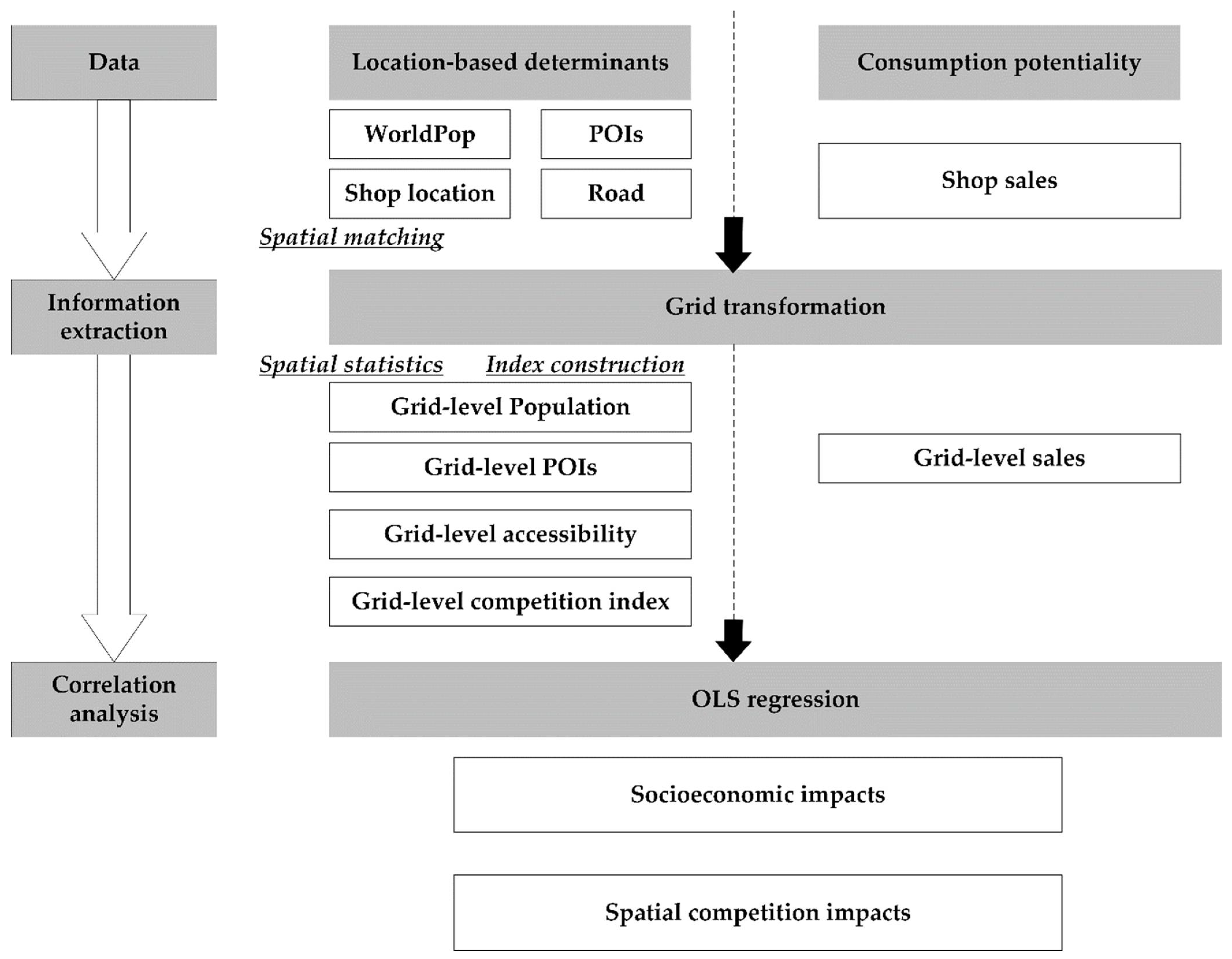
Figure 2 describes the flowchart of the method, which includes three main steps: (1) Data preparation and preprocessing. In this step, the population data of Guiyang City were extracted from the WordPop dataset; POI data of each category were extracted separately from the POI dataset; road data for Guiyang City were obtained; location data and sales data for retail shops with “stable” sales performance were obtained; the georeferencing of the above dataset was unified as WGS-84. (2) Grid-based index construction. In this step, a grid transformation strategy was conducted to organize all the variables into a grid level, and a location-based competition index was built according to the spatial relationship of these shops. (3) Correlation analysis through OLS regression. In this step, all the socioeconomic variables and spatial competition metrics were set as the input variables, and grid-level sales was set as the output variable. Through the regression, the impacts of these variables on consumption potentiality can be determined and explained.
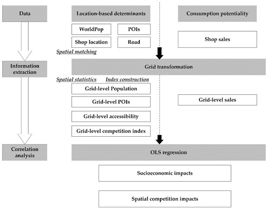
Figure 2.
Flowchart of the study.
3.2. Construction of Socioeconomic Indexes
3.2.1. Grid-Division Processing of Retail Shops
To capture the stable consumption potentiality of Guiyang Region for the execution of long-term business strategies, we excluded “temporary” retail shops with less than 12 months of sales data during the 24-month period:
where denotes the selected shops and denotes the number of months when shop i has effective sales (larger than 0). A total of 12,500 retail shops were finally selected as our main study objects. For these selected retail shops, we adopted their monthly average sales to represent the regular sales performance:
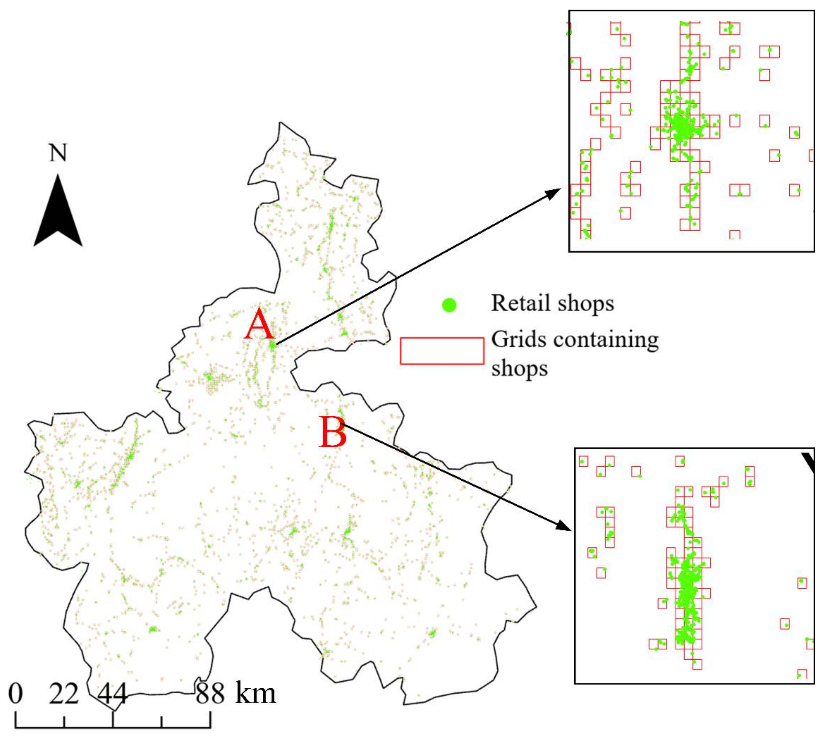
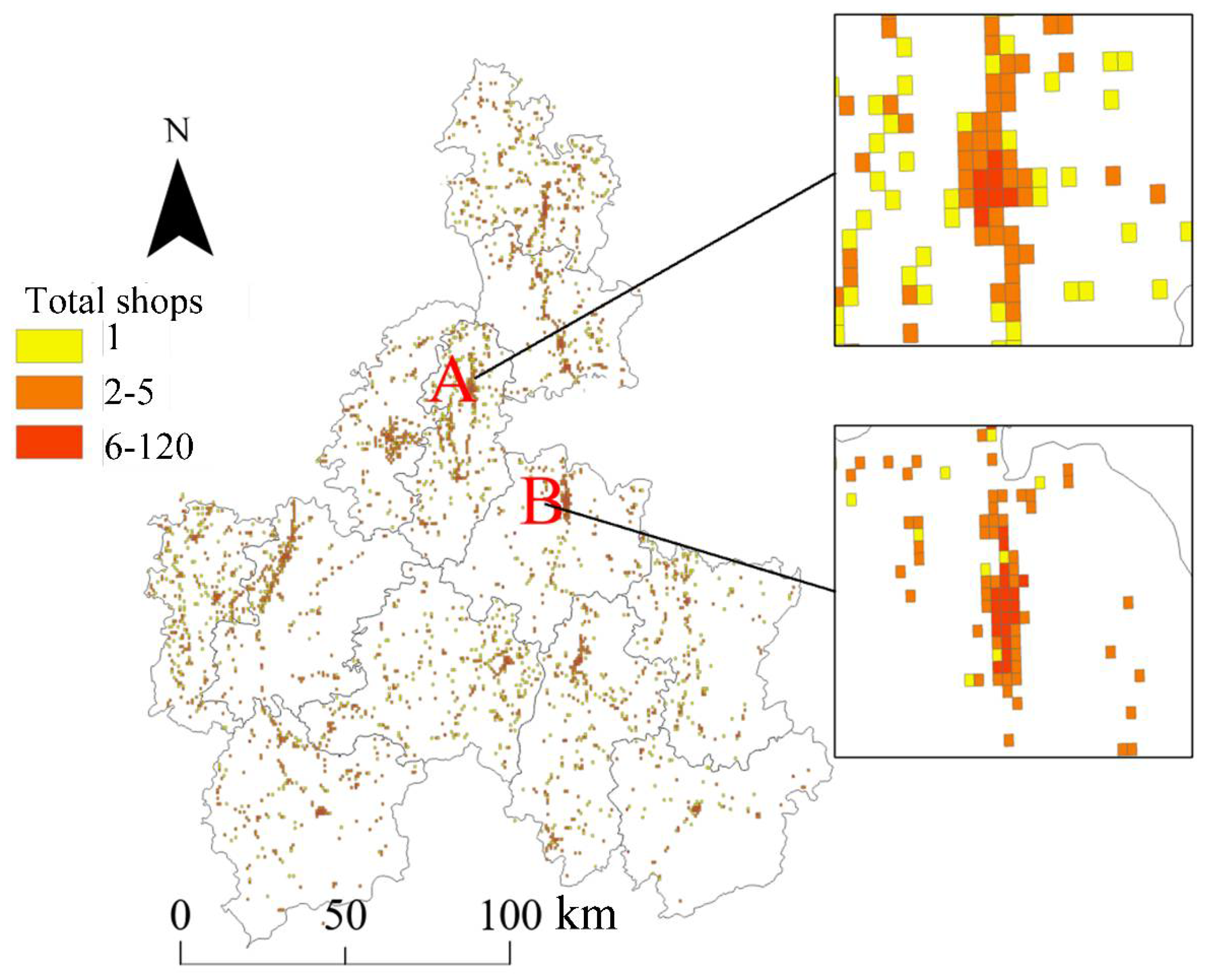
where denotes the sales of shop in month ; denotes the average sales of shop in months with effective sales. Figure 3 shows the spatial distribution of these selected retail shops. We choose two sample regions, A and B, located in Guiding County and Duyun County, respectively, to show the details of shop distribution. An aggregation trend of retail shops can be found in the center of the two counties.
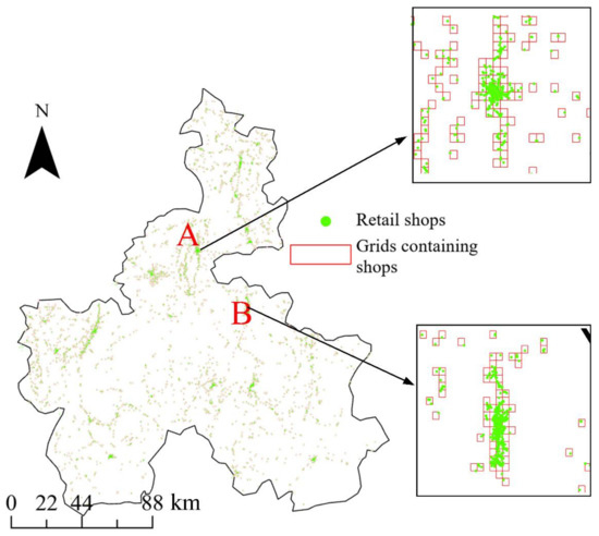
Figure 3.
Distribution of retail shops and grids containing retail shops. A and B denote two sample regions Guiding County and Duyun County, respectively.
Previous work has demonstrated that the consumption potentiality of retail shops can be highly influenced by human activities within a walkable distance (e.g., 500 m in Guizhou). Moreover, previous works have proposed a grid-division strategy to aggregate the retail shops’ sales performance and human activities. We also adopt this strategy in this study and form our data into a grid level. Figure 3 shows the distribution of grids, where the grids without retail sales were removed. We aggregate the retail sales into each grid:
where denotes the grid; denotes the number of shops located in grid ; denotes the average sales of shop , which is in grid ; and denotes the grid-level retail sales in grid .
3.2.2. Grid-Division Processing of POI Data
In our original dataset, the POI data can be divided into 21 categories according to their functional types. In the study area, the data volume of several kinds of POIs data can be small and distributed far from retail shops. For these POIs, their impacts on retail shops’ sales performance can be limited. Our previous work has demonstrated that the consumption potentiality of retail shops can be highly influenced by nearby facilities within approximately 500 m [19,32]. Therefore, we chose 500 m (spheroid-based distance) as a threshold to find POIs that are located far from retail shops. We calculated the distance of each POI to its nearest retail shop and grouped the information according to their types. Table 1 shows the results.

Table 1.
Nine POI categories within grids containing retail shops.
POIs, which can be divided into 15 types, can be found within 500 m of retail shops. However, the number of 6 kinds of POIs is quite small, ranging from 20 to 109, which is far smaller than the number of POIs. Considering these shops cannot cause much impact on most retail shops, we eliminated these POIs from our dataset. Finally, we chose 9 kinds of POIs, with a total number of 76,562, as the candidate variables, which were further adopted. Table 1 shows the retail types of the 9 POI categories.
The selected POIs were summarized into a grid level through spatial matching with grids:
where denotes the category of POIs; denotes the th grid; denotes the th POI of category located in grid ; denotes the number of POIs of category located in grid ; and denotes the total number of POIs of category located in grid .
3.2.3. Grid-Division Processing of Other Indexes
To obtain the grid-level population distribution information, the WorldPop 2015 dataset and WorldPop 2016 dataset at resolution were resampled into resolution. These datasets were then matched with the grids created in the above sections. Then, we calculated the average population data of each grid:
where denotes the population of the th grid derived from the resampled WorldPop 2015 data set; denotes the population of the th grid derived from the resampled WorldPop-2016 dataset; and denotes the average grid-level population in the th grid.
We performed the spatial matching of road data derived from the OSM dataset with grids and clipped the road data using the boundary of grids. Then, all the road parts located in each grid were summarized:
where denotes the th part of the road located in the th grid; denotes the length of road , which is totally located in grid ; and denotes the total length of roads located in grid .
We summarized the total area of geographic barriers in each grid:
where denotes the th part of geographic barriers located in the th grid; denotes the area of barrier , which is totally located in grid ; and denotes the total area of geographic barriers located in grid .
3.3. Construction of Competition Indexes
Besides socioeconomic factors, the spatial distribution of retail shops will cast impacts on consumption potentiality. According to previous research, the sales performance of retail shops in a region can suffer impacts from retail shops located in nearby regions. By adopting a grid-based method, Ouyang [33] pointed out that competition exists between retail shops in a grid and other retail shops distributed in nearby grids, and the competition is negatively correlated with the distance of these retail shops from the central grid.
To prove the idea proposed in previous studies, we proposed several indexes based on the number and spatial proximity of these shops. We built two types of indexes: (1) a grid-based shop ratio (2) a grid-based shop proximity.
3.3.1. Number-Based Shop Ratio Index
Considering that the number of retail shops is highly correlated with socioeconomic factors in each grid and cannot reflect the competition ability in each grid, we did not adopt the shop numbers directly. Instead, we built an index according to the number of retail shops distributed in each grid and nearby grids to examine if the retail shops in nearby grids will cause an impact on the consumption potentiality of the center grid.
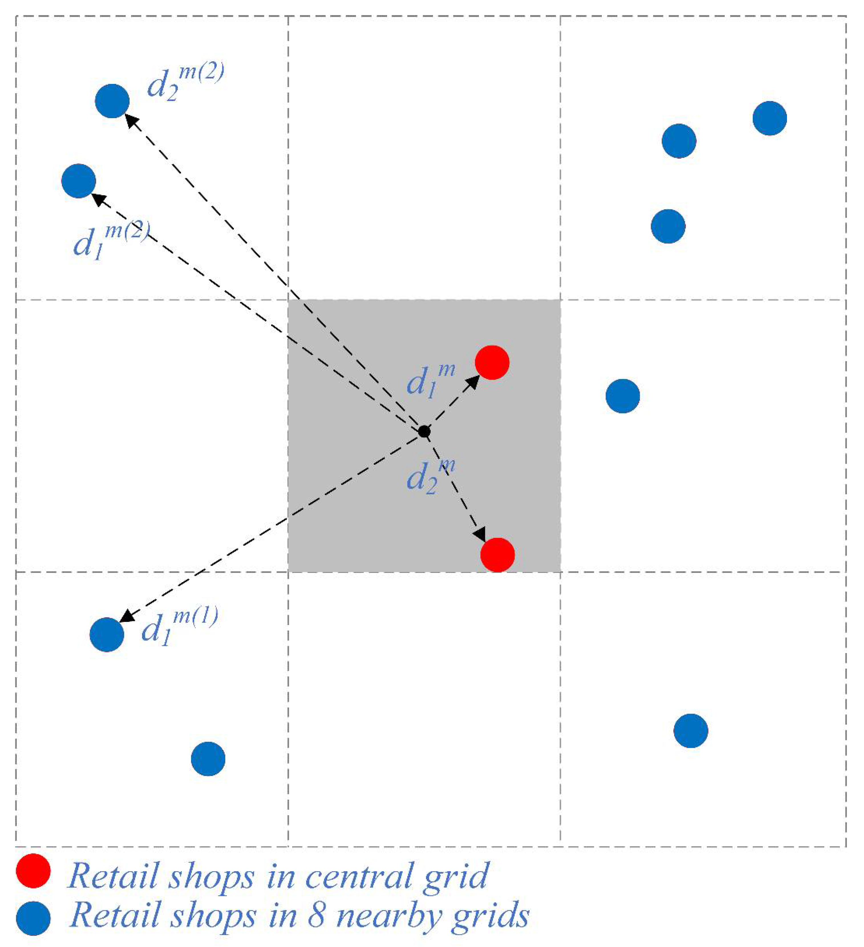
First, we calculated the number of retail shops in the center grid. Second, we calculated the number of retail shops distributed in eight nearby grids, as shown in Figure 4, and then we summed up these values. Finally, the number-based competition index was represented by the ratio of center-grid retail shops to nearby-grid retail shops:
where denotes the total number of retail shops located in the th grid; denotes one of the eight grids near grid ; and denotes the number-based competition index in the th grid. This index provides information on how important the retail shops are in each region.

Figure 4.
Spatial proximity of retail shops in the central grid and in eight nearby grids. Red points denote retail shops in central grid (gray background); blue points denote retail shops in nearby grids; denotes the distance of the central point to shop , which is located in central grid; denotes the distance of the central point to shop , which is in one of the nearby grids .
3.3.2. Distance-Based Shop Proximity Index
Besides the number of retail shops, previous research documented that the spatial proximity of nearby retail shops, which can be measured by distance, can cause impacts on the sales performance of shops in the center grid. In the research of [19], the distance between retail shops was found to be positively correlated with the competition. Specifically, the closer these shops are to the central grid, the lower the sales performance of shops near the central grid, due to strong competition. However, this thought has not been discussed thoroughly, especially when socioeconomic factors are controlled.
Therefore, we designed a distance-based index to measure the spatial proximity of retail shops in nearby grids to the central grid. Unlike the method proposed in previous studies, which calculated the distance between two retail shops, we built our index according to the distance between each retail shop and the central point of the study grid. This approach cannot only reduce the calculation complexity, but also better describe the situation when only one retail shop is present.
The central point of each grid was first determined. Then, the average distance from the central point to retail shops located in the grid and in eight nearby grids was calculated, which is formulated as:
where denotes the distance of the central point to shop , which is in grid ; denotes the total number of retail shops in grid ; denotes the average distance from the central point to all the shops located in grid . Similarly, we calculated the average distance from the central point to shops located in eight nearby grids:
where denotes the distance of the central point to shop , which is in one of the nearby grids ; denotes the total number of retail shops in grid ; and denotes the average distance from the central point to retail shops located in eight nearby grids.
3.4. Baseline Regression
The OLS regression model was adopted to analyze the relationship between two kinds of determinants, including socioeconomic factors and competition index, and grid-level sales performance. The OLS model has been widely used in socioeconomic studies, including the assessment of GDP growth [34], CO2 emission [35], electricity consumption [36], and COVID-19 vaccination rates [37]. It should be mentioned that some spatial regression models, such as geographically weighted regression (GWR) and conditional autoregressive models (CAM), have been widely used to model the spatial correlation and neighborhood effects in geographic studies and were proven to be more accurate than OLS in the estimation or prediction of tasks [38]. However, we hope to explore more general rules in the distribution of retail sales and to find out how retail sales react when some spatial factors change. Therefore, we believe that OLS is more suitable in this study than spatial regression models.
In this study, the input variables of OLS include competition indexes and socioeconomic factors. The output variable of the OLS model is the grid-level sales performance of each grid. The analysis of the OLS model is performed through the following steps: (1) The calculation of output variable—grid-based retail sales—which is derived from the sales of retail shops located within each grid. (2) The calculation of control variables, including grid-based POIs, grid-based population, and grid-based road length. These variables are the normally used socioeconomic variables, and they can be derived through spatial statistics. (3) The calculation of interest variables, including a ratio-based competition index and two distance-based competition indexes, describes the spatial proximity of retail shops within the grids. (4) The correlation analysis of input variables and output variables through OLS. We use a simplified baseline regression to explain how we design the OLS model:
where GSD denotes the grid-based socioeconomic indexes, including grid-based POIs (), grid-based population (), and grid-based road length (). denotes the grid-based competition indexes, including ratio-based competition index () and distance-based competition indexes ( and ). denotes the coefficients, and denotes the constant term.
4. Results
4.1. Grid-Based Shop Number and Sales Performance
4.1.1. Spatial Distribution of Retail Shops within Grids
Figure 5 shows the distribution of retail shops, in which three grid colors are used to distinguish the number of shops within each grid. The number of shops ranges from 1 to 120. Red grids (more than five retail shops) are mainly distributed in the northwestern counties of Qiannan, including Longli County, Guiding County, and Changshun County. This result indicates that retail shops in these regions are more likely to be concentrated together than those in southeastern counties like Shandu County, Dushan County, and Libo County. Two sample regions, A and B, in Guiding County and Duyun County, respectively, are selected to show the details of the shop distribution. Most red grids show a concentrated pattern in the city center, whereas yellow grids and orange grids (a small number of shops) are dispersed far from the city center.

Figure 5.
Number of shops in each grid.
4.1.2. Distribution of Grid-Level Total Retail Sales
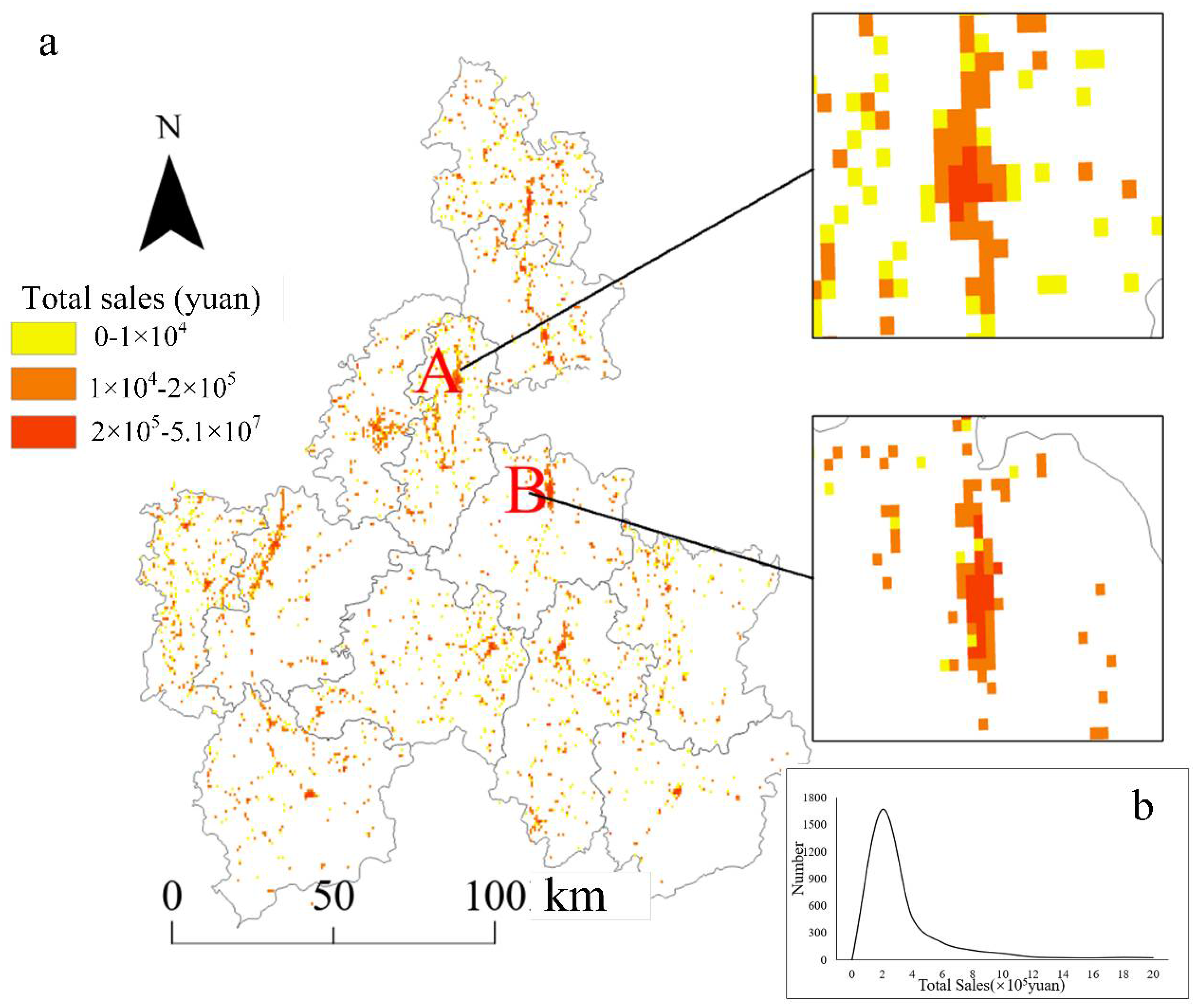
As to the grid-level retail sales, which range from and are represented in different colors in Figure 6a, the grids with high retail sales are also concentrated in the northwestern counties of Qiannan, including Longli County, Guiding County, and Changshun County. The pattern shows that these retail concentrating regions can normally attract high marketing sales, like sample regions A and B.

Figure 6.
(a) Spatial distribution of total retail sales in each grid. (b) Relationship curve of the number of shops and total retail sales in the grid scale.
We use a curve to find out the relationship between grid-level retail sales and the number of grids, which shows a normal distribution pattern in Figure 6b. The results show that the retail sales for most grids are distributed from per month, which reflects the consumption level of most regions in Qiannan County. A few grids with high retail sales, larger than per month, are mainly distributed in the city center of the northwestern counties.
4.2. Grid-Based Socioeconomic Determinants
4.2.1. Distribution of Grid-Level Population Data
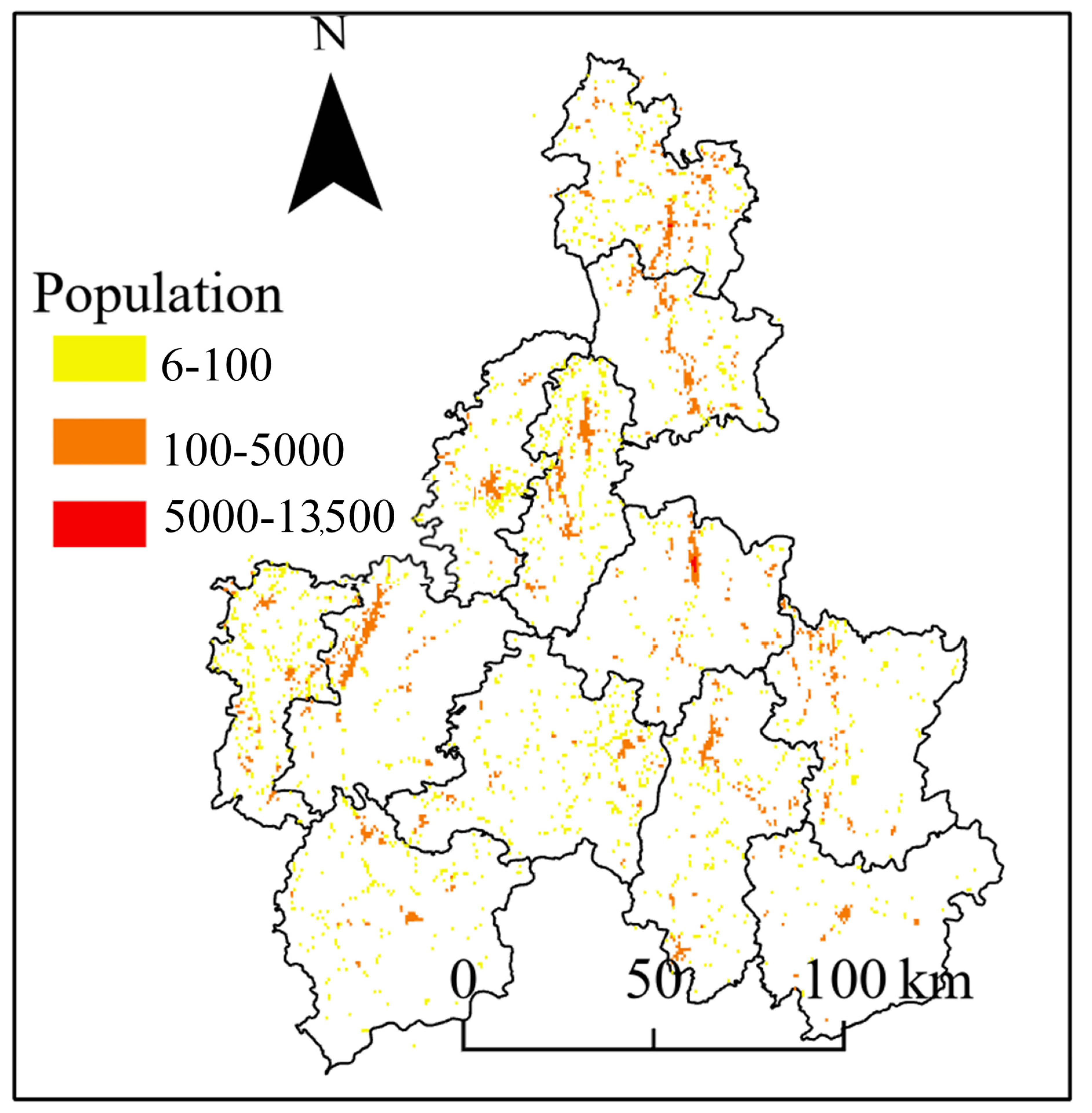
Figure 7 shows the distribution of the grid-level population, ranging from 6 to 13,505. Grids with high values, specifically larger than 5000, are mainly distributed in the northern and northwestern counties, including Wengan County, Longli County, Guiding County, Huishui County, and Changshun County.
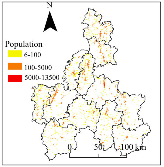
Figure 7.
Distribution of grid-level population data.
4.2.2. Grid-Based POI Distribution
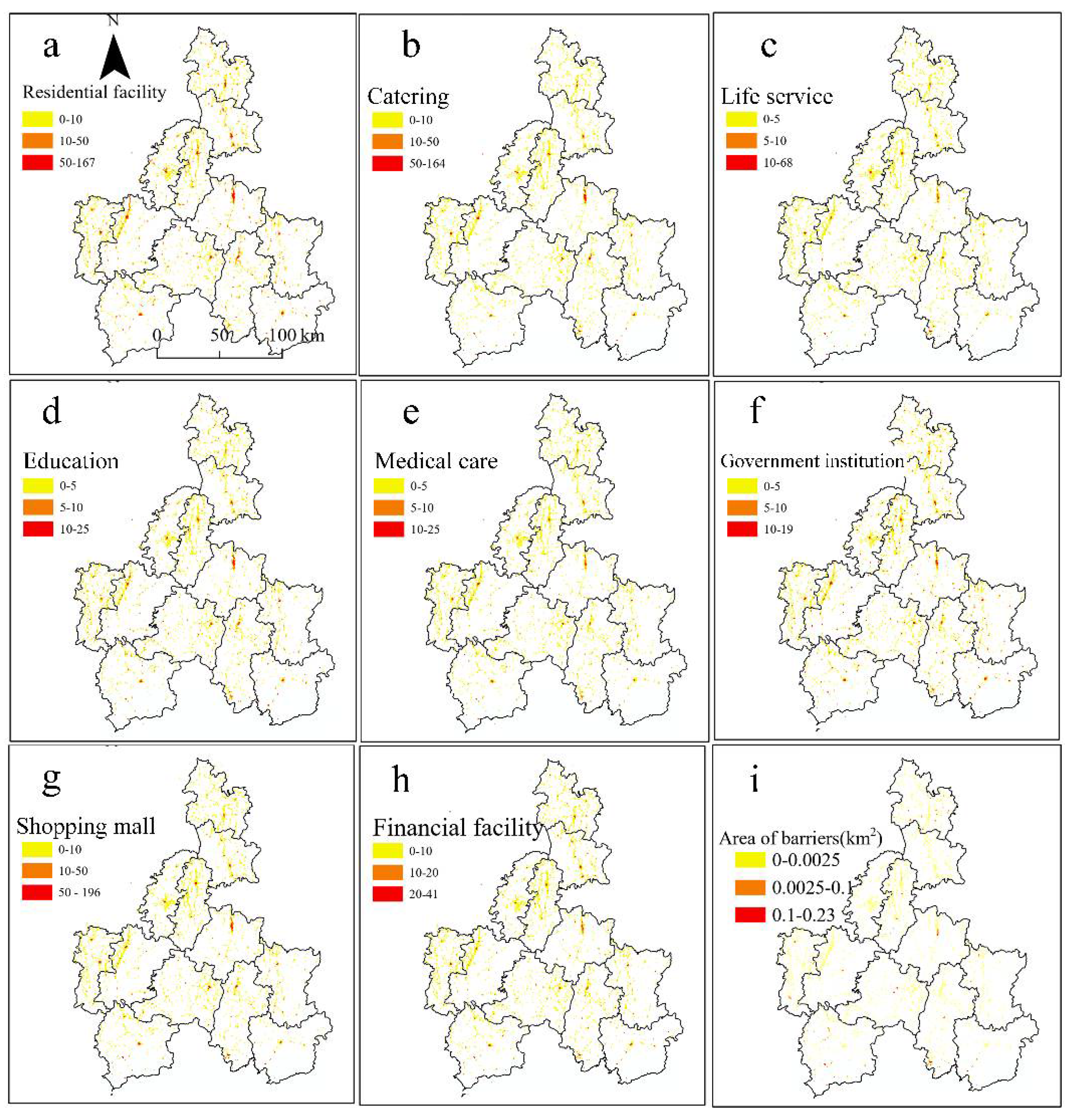
Figure 8a–h shows the distribution of grid-level POI data and the area of barriers. As shown in Figure 8a, the number of residential facilities ranges from 0–167, where most high value grids are concentrated in the northern and northwestern counties. This pattern is similar with that of the distribution of retail sales. The number of catering facilities ranges from 0–164, with high-value grids concentrated in Duyun County and Dushan County (Figure 8b). Shopping malls (Figure 8g) and financial facilities (Figure 8h) show a similar pattern. The number of life service shops ranges from 0–68; the number of education facilities ranges from 0–25; and the number of medical facilities ranges from 0–25. These three kinds of POIs show a similar pattern, with high-value grids concentrated in Duyun County, Longli County, and Guiding County. The number of government institutions ranges from 0–19, and they are dispersedly distributed in most regions. The area of barriers, which ranges from 0–0.23, shows a similar pattern.
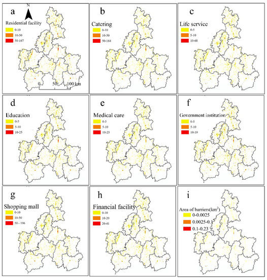
Figure 8.
(a–h) Distribution of POI data and (i) area of geographic barriers in grid scale.
4.3. Grid-Based Competition Index
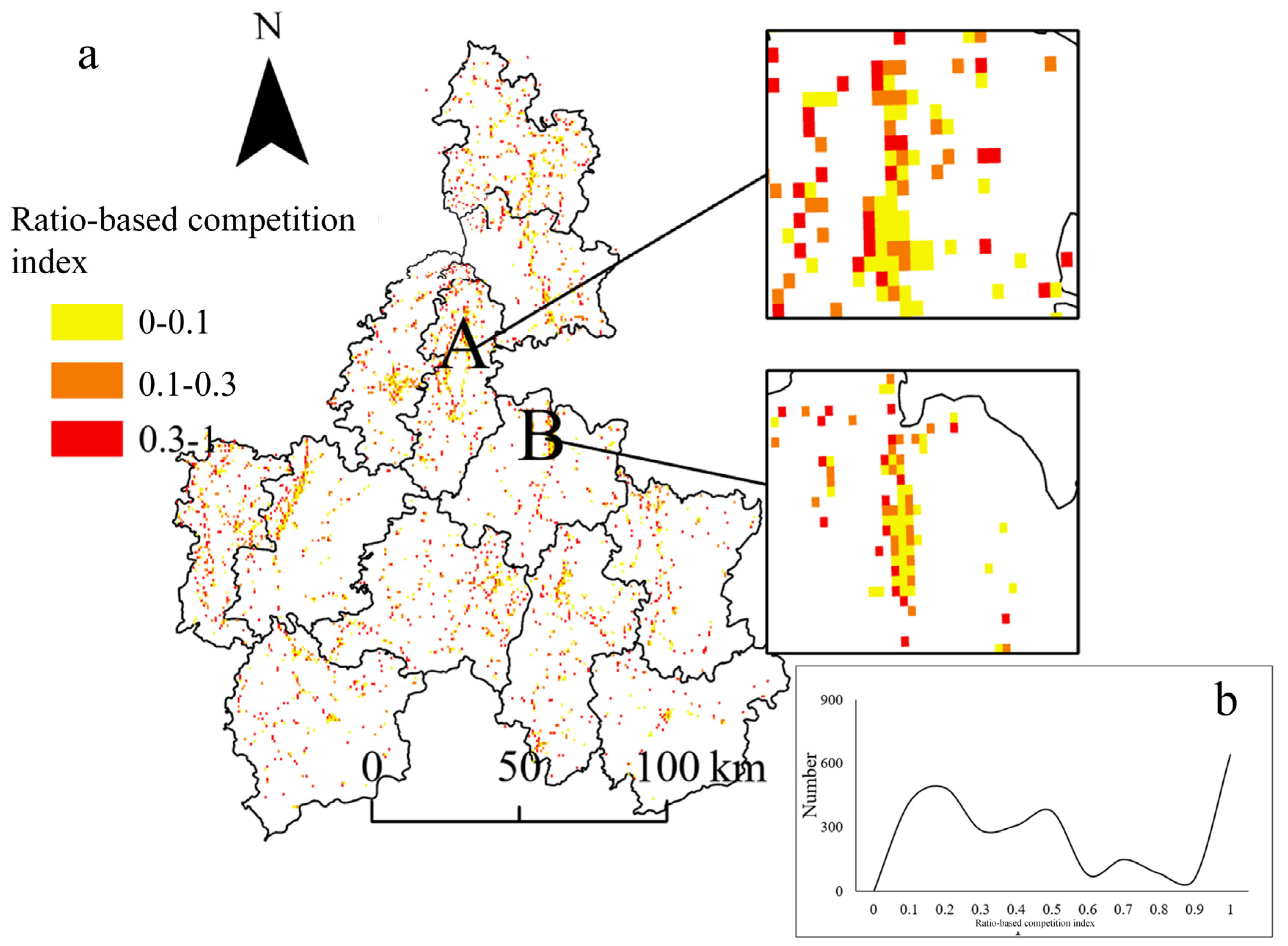
4.3.1. Ratio-Based Competition Index
Figure 9a shows the distribution of the ratio-based competition index, ranging from 0–1. High-value grids with indexes larger than 0.3 are dispersedly distributed across the whole Qiannan City. However, the value of grids in the city center of retail concentrating counties, such as Guiding County, Longli County, and Huishui County, is small (<0.1). The enlarged views of sample regions A and B reveal the pattern. We further present the relationship between the ratio-based competition index and the number of grids in a formula, as shown in Figure 9b. The results show that the value of most grids is distributed between 0.1–0.5 and 0.9–1, whereas only a few grids are located in sections 0.6–0.9. The results potentially reveal a distribution pattern for the retail industry in Qiannan: most retail shops are either concentrated together, or are totally isolated from one another.
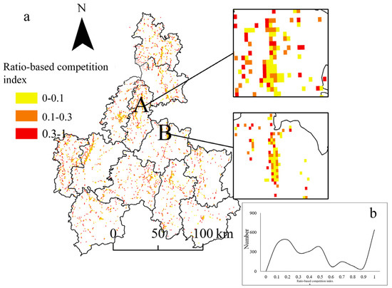
Figure 9.
(a) Distribution of the ratio-based competition index. (b) Relationship curve of the ratio-based competition index and the number of shops in the grid scale.
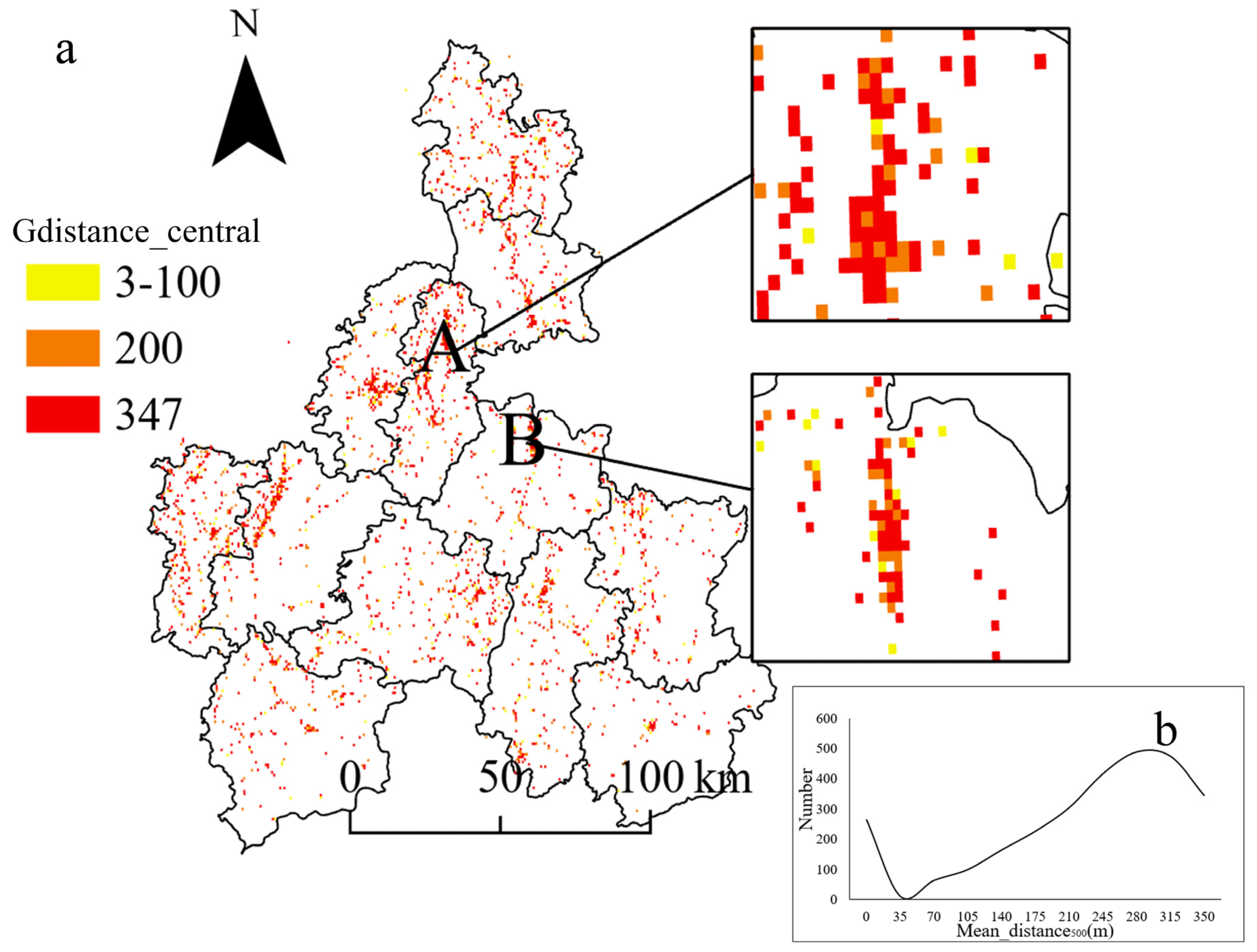
4.3.2. Distance-Based Shop Proximity Index
Figure 10 and Figure 11 show the distance-based shop proximity indexes, including and , respectively. , which denotes the average distance from the grid center to retail shops within each grid, ranges from 3–347 m, with high-value grids concentrated in the city center of the northern and northwestern counties, like region A and region B. In Figure 10b, we present the relationship between and the number of grids by using a formula. The grid number shows a decreasing pattern, with between 0–35 m and larger than 315 m, and an increasing pattern, with between 35–315 m.
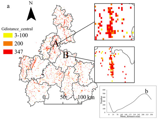
Figure 10.
(a) Distribution of the central grid distance-based competition index. (b) Relationship curve of the central grid distance-based competition index and the number of shops in the grid scale.
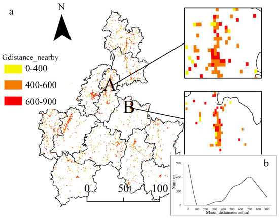
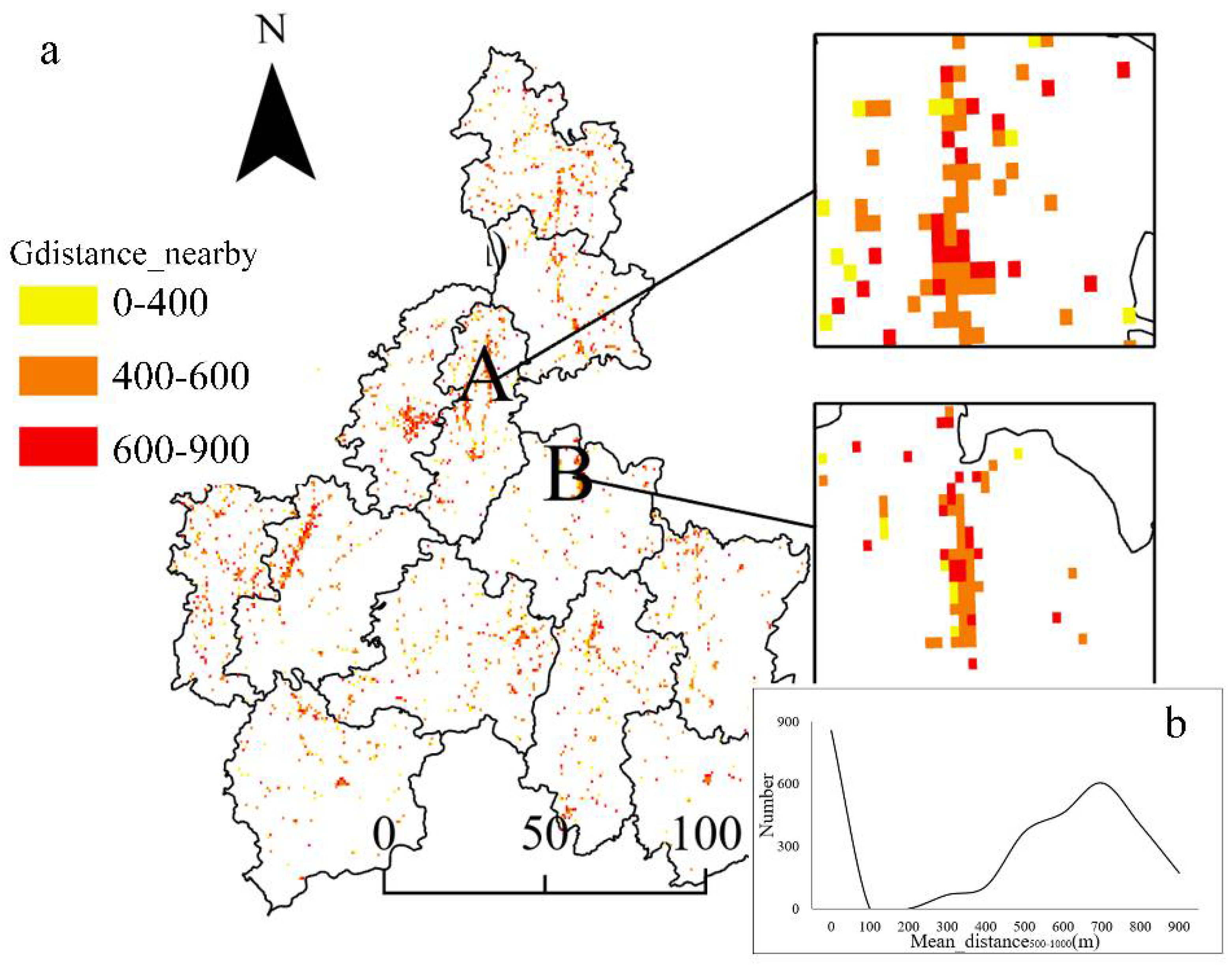
Figure 11.
(a) Distribution of the nearby grids distance-based competition index. (b) Relationship curve of nearby grids distance-based competition index and the number of shops in the grid scale.
As for , which ranges between 0–900 m, grids with high values are dispersed across Qiannan City (Figure 11a). Slightly different from the pattern of , the grid values of in the city center of the northwestern counties are mostly distributed in the middle range (400–600 m), resulting from the concentrated pattern of retail sales in the whole region. Figure 11b shows the relationship between and grid number, which reflects an increasing pattern, with between 465–900 m, and a decreasing trend, with between 700–900 m.
4.4. Regression Results
4.4.1. Correlation Test
Table 2 displays the correlations among the 17 variables in this paper. As the table shows, all the correlations among the independent variables and dependent variable are positive and significant, suggesting that these independent variables likely influence grid-based shop sales.
Table 2.
Correlations among the variables.
4.4.2. Effects of Socioeconomic Indexes and Shop Ratio on Sales Performance
Table 3 shows the results of multiple linear regression involving the grid-based spatial competition and socioeconomic determinants and the grid-based shop sales. The results indicate that the model fits well regarding the relationship between the independent variables and grid-based shop sales ().
Table 3.
Regression results of socioeconomic indexes and shop ratio on sales performance.
Table 3 shows that the grid-based shop sales will have moderate growth with population increases (). Road length has a positive effect on shop sales ), which demonstrates that spatial accessibility has a positive impact on regional consumption potentiality. Table 3 also shows that some POIs in the grid have significantly positive effects on grid-based shop sales, including the number of schools, residential communities, governmental agencies, financial services, and life services. However, the number of medical care facilities, the number of catering facilities, the location of mountains, and the number of supermarkets in the grid have negative impacts on grid-based shop sales. In particular, the result regarding the location of mountains indicates that spatial obstacles have a detrimental effect on regional economic benefits, which supports the findings in previous studies [39].
As for the competition index, we mainly focus on shop ratio in this section. The results show that the grid-based shop ratio has a significantly positive impact on grid-based shop sales (). Thus, the fewer shops located near the targeted grid, the higher the shop sales in the targeted grid. This result supports the cannibalization effect of stores in adjacent areas, as proposed by Guler [40].
4.4.3. Effects of Distance Metrics on Sales Performance
Competition effects are not only caused by the number of surrounding shops, but also by their distances to the targeted area. To investigate the spatial clustering in a commercial region, we considered two distance-based indexes and added them simultaneously into our regression model. Table 4 shows the results.
Table 4.
Regression results of the effects of distance metrics on sales performance.
The decentralization of the shops in one area has a marginally positive effect on grid-based shop sales (), and the decentralization of the shops in surrounding areas has a significantly positive effect on the dependent variable (). These findings indicate that the lower the clustering of the shops in the targeted area or its surrounding area is, the higher the financial benefits of the shops in this area. Table 4 demonstrates that grid-based shop distribution isolation (shop ratio) has a positive effect on shop sales in one area ().
As shown in Table 4, the influences of population, road network, and POIs on shop sales are relatively stable compared with the results shown in Table 3. The results again demonstrated the reliability of our findings obtained in Section 4.1.1; hence, we will not dwell on them in this section.
4.4.4. Effects of Squared Distance Metrics on Sales Performance
In the last section, the findings indicate that the spatial decentralization of the shops’ location may contribute to the sales in this area. However, in relation to other shops, is the greater the distance the better? To answer this question, we added the squared mean distances of the shops in this area, and its surrounding areas, from their location to the central point of the grid to our regression. Table 5 shows the results.
Table 5.
Regression results of squared distance metrics on sales performance.
Table 5 shows that the squared mean distances of the shops in the area () and the surrounding areas () are negatively correlated with regional sales, indicating that the influence of spatial proximity to the regional shop sales follows an inverted U-shaped relationship. The findings indicate thresholds for the mean distances of intra-regional shops and surrounding shops. By conducting the extreme value calculation method [41], we obtained the thresholds of 226.19 m and 514.85 m. Our findings have enriched the previous findings about the positive effect of distance [40].
The patterns of the influences of the other variables to regional consumption are consistent with the findings in Section 4.4.1 and Section 4.4.2, which also demonstrate the robustness of our previous findings.
5. Discussion
5.1. Robustness Check
Besides grid-level total consumption potentiality, per capita retail sales is important for retail trade [42,43]. Therefore, we represented the total consumption sales with per capita sales, which is calculated by:
where denotes per capita sales in the th grid. The new regression results are compared with the regression results of . Table 6 presents the results.
Table 6.
Robustness check using per capita sales.
The comparison of column 1 and column 2 in Table 6 shows a high similarity between the two regression results in the competition indexes. Column 2 shows that the shop ratio is positively correlated with per capita sales (), indicating that the fewer the shops located near the targeted grid, the higher the per capita sales in the targeted grid. The phenomenon may imply that the isolation of retail shops may stimulate consumers’ willingness to spend more in other places. The decentralization of the shops in each grid is positively correlated with per capita sales, as well as the decentralization of the shops in surrounding grids. The squared distances of shops are negatively correlated with per capita sales. The above findings are similar with that of total sales in Table 5.
Regarding socioeconomic factors, the number of catering facilities and shopping malls is negatively correlated with per capita sales. Moreover, the number of education facilities, financial services, and government institutions is positively correlated with per capita sales, which is similar to the relationship with total retail sales. However, the number of life-service facilities is negatively correlated with per capita sales, and the number of medical care centers is positively correlated with per capita sales, unlike the relationship with total sales. Grid-based road length and share of barriers are not significantly correlated with per capita sales.
5.2. Multicollinearity Check
We performed a multicollinearity check based on the variance inflation factor (VIF) of these variables. Multicollinearity is thought to exist among variables with VIF values larger than 10 [44]. Table 7 shows the VIF of variables adopted in this study.
Table 7.
VIFs of the independent variables.
The results indicate that multicollinearity does not exist among our interest variables (Gshop_ratio, Gdistance_central, Gdistance_nearby, Gdistance_central_square, and Gdistance_nearby_square) and other control variables, since their VIF values are all smaller than 10. There is just one exception of our control variable—GPOIs residential—in which the VIF is 12.402; this result is consistent with the correlations among GPOIs residential and other POIs, as shown in Table 2. We determined to use lasso regression, which is commonly used to deal with multicollinearity problems [45], to find out whether GPOIs residential will affect our results. Table 6. shows the results of lasso regression, where we can see that our variables of interest, Gshop_ratio, Gdistance_central, and Gdistance_nearby, are positively correlated with Gsales. Meanwhile, Gdistance_central_square and Gdistance_nearby_square are negatively correlated with Gsales. The results indicate that the correlativity between our interest variables and grid-based retail sales does not suffer any influence from the multicollinearity of GPOIs residential.
5.3. Limitations and Future Work
The current study has several limitations that need to be addressed in future studies.
First, store attributes, such as floor space, number of employees, and customer service quality, were not considered in this study. These characteristics may play an important role in regional consumption potentiality [46], but we were not able to use them in the regression due to lacking data. In future studies, shop-related information needs to be collected and included in the regression.
Second, information on human activities was not adopted in the current study. Regional consumption is not only correlated with a stable urban environment, but is also highly impacted by changeable human activities near the region. The location information for consumers can be difficult to obtain, considering the concerns for privacy protection. However, the emergence of location-based social media data, which have been used in consumption prediction, may provide a potential solution for this issue. In future studies, social media data can be utilized to reflect the consumption preferences and mobility of consumers and to provide supplementary information for human activities. This information will also support in-depth research on dynamic sales changes.
Third, the impacts of the spatial proximity of retail shops on regional sales performance need to be further studied using a better method of building competition indexes. Although we built two indexes and successfully found that the spatial distribution of retail shops has great impacts on retail shops, the mechanism is unclear. Moreover, overlaps exist between the two indexes. Future studies, therefore, may devote their efforts to creating a new index that can combine these two aspects and better describe the spatial proximity of retail shops. The new index can help determine why the impact follows an inverted U-shape, which is an interesting and important phenomenon to be explored.
6. Conclusions
The development of the Chinese economy has brought a huge opportunity for the retail industry [47]. Under the new circumstances, retail managers should understand the relationship between the urban environment and regional consumption potentiality to achieve sustainable development goals. This study adopted a statistical model to explore the relationship between spatial proximity of retail shops and regional retail sales through a study of 12,500 retail shops in Qiannan, China. Several conclusions can be drawn.
- (1)
- Several socioeconomic factors are important in determining regional consumption potentiality. Regional population, road length, and the number of POIs (i.e., education facilities, life services, financial services, government institutions, and residential facilities) are significantly and positively correlated with consumption potentiality. By contrast, the area of geographic barriers and the number of three kinds of POIs (i.e., catering facilities, shopping malls, and medical-care institutions) are significantly and negatively correlated with consumption potentiality.
- (2)
- The spatial proximity of retail shops will cause competition, which will cause impacts on regional consumption. Grid-based shop distribution isolation (shop ratio) has a significantly positive effect on shop sales in one area. The decentralization of the shops in one area has a marginally positive effect on grid-based shop sales, and the decentralization of the shops in surrounding areas has a significantly positive effect on the dependent variable.
- (3)
- The influence of spatial proximity to the regional shop sales follows an inverted U-shape. The findings indicate thresholds for the mean distances of intra-regional shops and surrounding shops, which are 226.19 m and 514.85 m, respectively.
Our study deepens our understanding on the relationship between location-based socioeconomic factors and micro-level retail sales, which may provide reliable information and practical guidance for the sustainable development of the retail industry.
Author Contributions
Conceptualization, Wei Wang and Luyao Wang; methodology, Luyao Wang; validation, Wei Wang, Luyao Wang and Xu Wang; writing—original draft preparation, Wei Wang, Luyao Wang and Yankun Wang; revision process, Wei Wang, Luyao Wang, Yankun Wang and Xu Wang All authors have read and agreed to the published version of the manuscript.
Funding
This research was funded by the National Natural Science Foundation of China (NSFC) (Grant No. 42001389, 62102423, 72001046).
Institutional Review Board Statement
Not applicable.
Informed Consent Statement
Not applicable.
Data Availability Statement
Not applicable.
Acknowledgments
The authors thank Xiaoyu Long and Shengxiang Lv for their help during the data curation and analysis of this study.
Conflicts of Interest
The authors declare no conflict of interest.
References
- Wang, Q.; Zhang, F. What does the China’s economic recovery after COVID-19 pandemic mean for the economic growth and energy consumption of other countries? J. Clean. Prod. 2021, 295, 126265. [Google Scholar] [CrossRef]
- Jia, Z.; Wen, S.; Lin, B. The effects and reacts of COVID-19 pandemic and international oil price on energy, economy, and environment in China. Appl. Energy 2021, 302, 117612. [Google Scholar] [CrossRef]
- Statistics, N.B.O. China Economic Annual Report of 2021; The State Statistical Bureau: Beijing, China, 2022. [Google Scholar]
- Song, S. Street stall economy in China in the post-COVID-19 era: Dilemmas and regulatory suggestions. Res. Glob. 2020, 2, 100030. [Google Scholar] [CrossRef]
- Guo, F.; Huang, Y.; Wang, J.; Wang, X. The informal economy at times of COVID-19 pandemic. China Econ. Rev. 2022, 71, 101722. [Google Scholar] [CrossRef]
- Chen, H.; Qian, W.; Wen, Q. The impact of the COVID-19 pandemic on consumption: Learning from high-frequency transaction data. In AEA Papers and Proceedings; American Economic Association: Nashville, TN, USA, 2021; pp. 307–311. [Google Scholar]
- Lawson, R.M. The supply response of retail trading services to urban population growth in Ghana. In The Development of Indigenous Trade and Markets in West Africa; Routledge: London, UK, 2018; pp. 377–398. [Google Scholar]
- Rosenlund, J.; Nyblom, Å.; Ekholm, H.M.; Sörme, L. The emergence of food waste as an issue in Swedish retail. Br. Food J. 2020, 122, 3283–3296. [Google Scholar] [CrossRef]
- Punyatoya, P. Linking environmental awareness and perceived brand eco-friendliness to brand trust and purchase intention. Glob. Bus. Rev. 2014, 15, 279–289. [Google Scholar] [CrossRef]
- Jorgensen Zevenbergen, R. Young workers and their dispositions towards mathematics: Tensions of a mathematical habitus in the retail industry. Educ. Stud. Math. 2011, 76, 87–100. [Google Scholar] [CrossRef] [Green Version]
- Anagboso, M.; McLaren, C. The impact of the recession on retail sales volumes. Econ. Labour Mark. Rev. 2009, 3, 22–28. [Google Scholar] [CrossRef]
- Noble Jacob, D.K.K. An Effective Model for Predicting the Customer Churn in the Retail Sector Based on CRM. Des. Eng. 2021, 12627–12646. [Google Scholar]
- Kim, S.-S.; Lee, J.-H. How does corporate social responsibility affect asymmetric information: Evidence from Korean retail industry. J. Distrib. Sci. 2019, 17, 5–11. [Google Scholar]
- Plaza, A.G.; Saulais, L.; Blumenthal, D.; Delarue, J. Eating location as a reference point: Differences in hedonic evaluation of dishes according to consumption situation. Food Qual. Prefer. 2019, 78, 103738. [Google Scholar] [CrossRef]
- Robertson, D.A.; Lunn, P.D. The effect of spatial location of calorie information on choice, consumption and eye movements. Appetite 2020, 144, 104446. [Google Scholar] [CrossRef]
- Clarke, M.; Birkin, M. Spatial interaction models: From numerical experiments to commercial applications. Appl. Spat. Anal. Policy 2018, 11, 713–729. [Google Scholar] [CrossRef]
- Anderson, S.J.; Volker, J.X.; Phillips, M.D. Converse’s breaking-point model revised. J. Manag. Mark. Res. 2010, 3, 1. [Google Scholar]
- Wang, Y.; Jiang, W.; Liu, S.; Ye, X.; Wang, T. Evaluating trade areas using social media data with a calibrated huff model. ISPRS Int. J. Geo Inf. 2016, 5, 112. [Google Scholar] [CrossRef] [Green Version]
- Luyao, W.; Hong, F.; Yankun, W. Site Selection of Retail Shops Based on Spatial Accessibility and Hybrid BP Neural Network. Isprs Int. J. Geo Inf. 2018, 7, 202. [Google Scholar]
- Applebaum, W.; Cohen, S.B. The dynamics of store trading areas and market equilibrium. Ann. Assoc. Am. Geogr. 1961, 51, 73–101. [Google Scholar] [CrossRef]
- Wang, L.; Fan, H.; Wang, Y. Estimation of consumption potentiality using VIIRS night-time light data. PLoS ONE 2018, 13, e0206230. [Google Scholar] [CrossRef]
- Yuesong, T.; Chao, W. Problems and Countermeasures of Characteristic Development of Small Towns in Qiannan Prefecture. In Proceedings of International Symposium on Advancement of Construction Management and Real Estate; Springer: Singapore, 2018; pp. 151–158. [Google Scholar]
- Xiangmei, M.; Leping, T.; Chen, Y.; Lifeng, W. Forecast of annual water consumption in 31 regions of China considering GDP and population. Sustain. Prod. Consum. 2021, 27, 713–736. [Google Scholar] [CrossRef]
- Xiao, Y. Research on Spatial Pattern and Influencing Factors of Consumption Vitality in the Middle Areas Based on POI data—A Case Study of Hefei City. In Proceedings of International Conference on Decision Science & Management; Springer: Singapore, 2021; pp. 481–488. [Google Scholar]
- Hou, G.; Chen, L. Regional commercial center identification based on POI big data in China. Arab. J. Geosci. 2021, 14, 1–14. [Google Scholar] [CrossRef]
- Zhang, X.; Xu, Z. Functional coupling degree and human activity intensity of production–living–ecological space in underdeveloped regions in China: Case study of Guizhou Province. Land 2021, 10, 56. [Google Scholar] [CrossRef]
- Alghanim, A.; Jilani, M.; Bertolotto, M.; McArdle, G. Leveraging Road Characteristics and Contributor Behaviour for Assessing Road Type Quality in OSM. ISPRS Int. J. Geo Inf. 2021, 10, 436. [Google Scholar] [CrossRef]
- Wang, H.; Wang, J.; Yu, P.; Chen, X.; Wang, Z. Extraction and construction algorithm of traffic road network model based on OSM file. In Journal of Physics: Conference Series; IOP Publishing: Bristol, UK, 2021; Volume 1848, p. 012084. [Google Scholar]
- You, H.; Yang, J.; Xue, B.; Xiao, X.; Xia, J.; Jin, C.; Li, X. Spatial evolution of population change in Northeast China during 1992–2018. Sci. Total Environ. 2021, 776, 146023. [Google Scholar] [CrossRef]
- Tatem, A.J. WorldPop, open data for spatial demography. Sci. Data 2017, 4, 1–4. [Google Scholar] [CrossRef]
- Chen, B.; Xu, B.; Zhu, Z.; Yuan, C.; Suen, H.P.; Guo, J.; Xu, N.; Li, W.; Zhao, Y.; Yang, J. Stable classification with limited sample: Transferring a 30-m resolution sample set collected in 2015 to mapping 10-m resolution global land cover in 2017. Sci. Bull 2019, 64, 370–373. [Google Scholar]
- Wang, L.; Hong, F.; Gong, T. The Consumer Demand Estimating and Purchasing Strategies Optimizing of FMCG Retailers Based on Geographic Methods. Sustainability 2018, 10, 466. [Google Scholar] [CrossRef] [Green Version]
- Ouyang, J.; Fan, H.; Wang, L.; Yang, M.; Ma, Y. Site selection improvement of retailers based on spatial competition strategy and a double-channel convolutional neural network. ISPRS Int. J. Geo Inf. 2020, 9, 357. [Google Scholar] [CrossRef]
- Kwark, N.-S.; Lee, C. Asymmetric effects of financial conditions on GDP growth in Korea: A quantile regression analysis. Econ. Model. 2021, 94, 351–369. [Google Scholar] [CrossRef]
- Mohsin, M.; Naseem, S.; Sarfraz, M.; Azam, T. Assessing the effects of fuel energy consumption, foreign direct investment and GDP on CO2 emission: New data science evidence from Europe & Central Asia. Fuel 2022, 314, 123098. [Google Scholar]
- Kim, M.-J. Understanding the determinants on household electricity consumption in Korea: OLS regression and quantile regression. Electr. J. 2020, 33, 106802. [Google Scholar] [CrossRef]
- Guo, Y.; Kaniuka, A.R.; Gao, J.; Sims, O.T. An Epidemiologic Analysis of Associations between County-Level Per Capita Income, Unemployment Rate, and COVID-19 Vaccination Rates in the United States. Int. J. Environ. Res. Public Health 2022, 19, 1755. [Google Scholar] [CrossRef] [PubMed]
- Wu, C.; Kim, I.; Chung, H. The effects of built environment spatial variation on bike-sharing usage: A case study of Suzhou, China. Cities 2021, 110, 103063. [Google Scholar] [CrossRef]
- Saiz, A. The geographic determinants of housing supply. Q. J. Econ. 2010, 125, 1253–1296. [Google Scholar] [CrossRef] [Green Version]
- Guler, A.U. Inferring the economics of store density from closures: The Starbucks case. Mark. Sci. 2018, 37, 611–630. [Google Scholar] [CrossRef]
- Yao, F.; Wen, H.; Luan, J. CVaR measurement and operational risk management in commercial banks according to the peak value method of extreme value theory. Math. Comput. Model. 2013, 58, 15–27. [Google Scholar] [CrossRef]
- Ingene, C.A.; Yu, E.S. Environment determinants of total per capita retail sales in SMSAs. J. Reg. Anal. Policy 1982, 12, 52–61. [Google Scholar]
- Myran, D.T.; Smith, B.T.; Cantor, N.; Li, L.; Saha, S.; Paradis, C.; Jesseman, R.; Tanuseputro, P.; Hobin, E. Changes in the dollar value of per capita alcohol, essential, and non-essential retail sales in Canada during COVID-19. BMC Public Health 2021, 21, 1–9. [Google Scholar] [CrossRef] [PubMed]
- Salmerón Gómez, R.; García Pérez, J.; López Martín, M.D.; García, C.G. Collinearity diagnostic applied in ridge estimation through the variance inflation factor. J. Appl. Stat. 2015, 43, 1831–1849. [Google Scholar] [CrossRef]
- Shafiee, S.; Lied, L.M.; Burud, I.; Dieseth, J.A.; Lillemo, M. Sequential forward selection and support vector regression in comparison to LASSO regression for spring wheat yield prediction based on UAV imagery. Comput. Electron. Agric. 2021, 183, 106036. [Google Scholar] [CrossRef]
- Weitzel, W.; Schwartzkopf, A.B.; Peach, E.B. The influence of employee perceptions of customer service on retail store sales. J. Retail. 1989, 65, 27–40. [Google Scholar]
- Jin, X.; Bao, J.; Tang, C. Profiling and evaluating Chinese consumers regarding post-COVID-19 travel. Curr. Issues Tour. 2021, 25, 745–763. [Google Scholar] [CrossRef]
Publisher’s Note: MDPI stays neutral with regard to jurisdictional claims in published maps and institutional affiliations. |
© 2022 by the authors. Licensee MDPI, Basel, Switzerland. This article is an open access article distributed under the terms and conditions of the Creative Commons Attribution (CC BY) license (https://creativecommons.org/licenses/by/4.0/).