Article

Harmonizing Full and Partial Matching in Geospatial Conflation: A Unified Optimization Model

1
Department of Geography and Atmospheric Science, University of Kansas, Lawrence, KS 66045, USA
2
College of Automation, Wuhan University of Technology, Wuhan 430070, China
*
Author to whom correspondence should be addressed.
ISPRS Int. J. Geo-Inf. 2022, 11(7), 375; https://doi.org/10.3390/ijgi11070375
Submission received: 24 April 2022 / Revised: 22 June 2022 / Accepted: 4 July 2022 / Published: 6 July 2022

Abstract

:
Spatial data conflation is aimed at matching and merging objects in two datasets into a more comprehensive one. Starting from the “map assignment problem” in the 1980s, optimized conflation models treat feature matching as a natural optimization problem of minimizing certain metrics, such as the total discrepancy. One complication in optimized conflation is that heterogeneous datasets can represent geographic features differently. Features can correspond to target features in the other dataset either on a one-to-one basis (forming full matches) or on a many-to-one basis (forming partial matches). Traditional models consider either full matching or partial matches exclusively. This dichotomy has several issues. Firstly, full matching models are limited and cannot capture any partial match. Secondly, partial matching models treat full matches just as partial matches, and they are more prone to admit false matches. Thirdly, existing conflation models may introduce conflicting directional matches. This paper presents a new model that captures both full and partial matches simultaneously. This allows us to impose structural constraints differently on full/partial matches and enforce the consistency between directional matches. Experimental results show that the new model outperforms conventional optimized conflation models in terms of precision (89.2%), while achieving a similar recall (93.2%).

1. Introduction

A common requirement in many practical spatial analyses is to effectively combine information from different data sources. In transportation studies, public agencies such as U.S. Census provide road network data with rich socioeconomic information, while private companies and crowd-sourced GISs provide data with more detailed information about the infrastructure including speed limit, number of lanes, surface type, etc. In studying migration and historical trends, it is often necessary to combine GIS data from different points of time that do not align with each other. In all these cases, it is necessary for the analyst to reconcile data elements from different sources and combine them into a better dataset. This process is known as conflation.
Conceptually, conflation can be divided into two stages. The first stage is matching, in which GIS features corresponding to the same objects in reality are linked to each other. The second stage is merging, in which attributes and/or geometries are transferred from one dataset to another or merged to form a new dataset. Of the two stages, matching is often the more difficult task, as getting the match wrong will ruin the subsequent merging process. Moreover, complexities in GIS data can confuse computerized algorithms and incur wrong matches. Figure 1a presents the layout of road features of downtown Santa Barbara, CA from OpenStreetMap (OSM in green) and TIGER (in red), respectively. For the rest of the paper, we represent the OSM road network in green and the TIGER roads in red in the Figures. One can observe that there are large spatial offsets between corresponding features—large enough to cause problems if one uses standard GIS operations such as the nearest neighbor joins to match features. Bath St. in OSM would be matched to Curley Ave in TIGER. Likewise, Curley Ave. in OSM would be matched to Castillo St. in TIGER. Extracting correct matches is the prerequisite of successful conflation.
The notion of matching may not be as simple as it appears. The concept of identifying the corresponding features in the above example assumes that the two features represent the same object in its entirety. The correspondence here is a full match (or one-to-one match) and it is the simplest match relation. More complex relations exist. Figure 1b shows the same road network for another street block. East Anapamu Street was represented as a single polyline in the TIGER dataset but was split into two polylines by an unnamed road in the OSM dataset. Their matches (the blue arrows) are partial matches (also known as many-to-one matches). Partial matches are more complex with a greater number of possibilities. A street could be split into several parts, with some parts matched correctly and others matched incorrectly. Generally speaking, partial matches often result from a difference in the scale or level of detail [1]. As discussed in the next section, there are even more complex matching relations at the subfeature level.
Among the different match relations, full matches can be successfully handled by existing conflation algorithms such as the “map assignment problem” conceptualized in the 1980s. One shortcoming of these models is that they cannot capture partial matches and miss a portion of all matches. Partial matches can be problematic for some current conflation algorithms. Current partial matching algorithms either do not explicitly consider full matches or treat them as one partial match or two partial matches (in opposite directions). Due to their greater complexity, such treatments often incur higher false (positive) matches and lower precision compared with full matching algorithms.
In this paper, we take an optimization approach to conflation. Similar to the “map assignment problem”, we treat conflation as a problem of minimizing total discrepancy or maximizing similarity. In particular, we present a unifying optimization model for conflation that simultaneously considers full and bidirectional partial matches. Unlike traditional optimized conflation models, we unify decisions about making full matches and partial matches in one model. We explicitly express full and partial matches with separate decision variables. This treatment makes it possible to prioritize full matches (because they are more reliable) while allowing partial matches at the same time. In addition, we impose new structural constraints to prevent conflicting matches in the two opposite directions of match. We also use a simple string distance to take advantage of street name information. Experimental results using comparable datasets show that the new model outperforms conventional optimized conflation models including the network-flow-based models as well as the classic assignment problem.
The rest of this paper is organized as follows. Section 2 presents a brief overview of conflation methods and the relevant literature. Section 3 presents the formulation of the proposed model and its design considerations. Section 4 presents the computational results obtained using two road network datasets for Santa Barbara, CA. We then conclude the paper with a summary of findings and suggest possible future research.

2. Background

Conflation is needed in a wide range of spatial analyses because spatial data about a phenomenon are often generated by different vendors and/or at different times. An example application of conflation is that of road networks. This is not only due to the great complexity of such networks but also because of their important functions as corridors of movement and a common reference system. Many sources provide road data, including public agencies, such as the U.S. Census, and private companies such as Here.com. Transportation research often requires rich information from all these sources. Combining historical administrative boundaries is another prominent application of conflation. The correct use of historical data requires identifying the changes over time and linking the regions that correspond to the same area at different periods of time. Owing to their potential utility, many conflation methods have been developed since the 1980s [2,3,4]. They have been used to conflate different types of features, including matching point features (e.g., gazettes [5]) and linear features (e.g., roads [6] and river networks), and areal features (e.g., building footprints and census tracts [7]), respectively.

2.1. Similarity Measures

Distances or similarity measures are common concepts underlying most conflation methods. They measure how different or similar two features are based on their geometries, attributes, and topological properties. For a comprehensive review of similarity measures in conflation, the reader is referred to [8]. Among the different measures of similarity, geometric similarity is by far the most widely used metric for geospatial conflation [8]. It can be calculated directly from the spatial displacement of vertices of two shapes. A widely used distance of this type is the Hausdorff distance. Given two features A and B (e.g., two polylines), the directed Hausdorff distance from A to B is h A , B = max p A min q B p q . This is the maximum offset from any point on feature A to feature B . If this distance is zero or near zero, obviously A either coincides with part of B or lies close to B . In other words, A is likely to correspond to part of B or belong to B . The full Hausdorff distance H A , B is defined to be the greater of the two directional Hausdorff distances h A , B and h B , A . If it is (near) zero, the two features belong to each other or are the same. Other distance functions, such as the Frechet distance and Turning Function distance have the additional capability of characterizing the difference in shape, but they are more computationally expensive. Some researchers compared two features by computing surrogate metrics such as length, size, and compactness, and then compared their differences based on such metrics.
Researchers have also compared features based on their differences in attributes such as street names. The authors of [9] used a Hamming distance to measure the difference of street names in addition to a displacement type distance metric (Hausdorff distance). The authors of [5] employed the Levenshtein distance to characterize the similarity of place names. Topological measures have also been used to compare two features based on contextual information, such as the number of edges to which a node is connected (i.e., its degree).

2.2. Extracting Match Relations

Effective conflation relies on the use of a good similarity measure. Additionally, a process is needed to select pairs of corresponding features to match based on their similarity. The simplest selection strategy is to assign each feature to candidate features in the other dataset purely based on their distances. This idea lies behind conflation methods that directly use standard GIS operations. Two types of GIS operations are often used in this context. The first is the nearest neighbor join (see [10] for a discussion). Here, a feature is assigned to the closest candidate (closest assignment). A related algorithm called k-Closest Pairs Queries (KCPQ) also exists in spatial database research [11], which finds the k pairs of matching features with the smallest distances. The second type of methods use buffer analysis (see e.g., [12]). Here, buffers for two features are generated first and the strength of association between them is measured by the amount of overlap between the buffer polygons. In a way, the buffer methods are a variant of the closest assignment strategy in which a distance threshold (i.e., the buffer radius) is used instead of comparing distances on a continuous scale.
Methods that purely rely on individual distances may work well if the two datasets involved are well-aligned. However, as shown in Figure 1a, these methods can be easily disrupted when any significant spatial displacements exist. Features may be assigned to incorrect candidates when using the closest assignment strategy; buffer overlays can incur multiple candidates meeting the threshold or no candidate at all. In general, these algorithms are “greedy” in nature, and once an erroneous match is made, it is difficult to rectify the error in the aftermath.
A more serious issue with the greedy strategy above is that it can generate inconsistent matches. As pointed out by [10], using nearest neighbor joins may generate transitive assignments. A feature A in dataset 1 may have some feature B on its right in dataset 2 as its closest feature (and therefore match under greedy assignment), but it may well be that feature B may have another feature C on its right in dataset 1 that is even closer. Therefore, the algorithm would assign A to B and then assign B to another feature C . This transitive assignment A B C is logically inconsistent. Under the full match assumption, this means that A is “equal” to B in dataset 2, but B is equal to something else (feature C ) in dataset 1.
To address the conflicts of nearest spatial joins, [10] proposed to compute certain confidence values for pairs of features (based on distances in competing alternatives). Several different rules were defined to choose matches, including using a threshold on the confidence value, using a proxy “probability” value, and picking the pair with the highest value and a “mutually nearest neighbor” method. More sophisticated match selection methods include [13], in which the authors used a logistic regression method to complement an optimization-based conflation model. These sophisticated match selection methods allow the scope of selection to be expanded to many features in the neighborhood.
To address the issues associated with spatial displacement, the U.S. Census developed the so-called rubber-sheeting procedure [14] while integrating their datasets with USGS data. It involves selecting a set of anchor points that represent prominent corresponding points (such as road junctions) from two datasets. It then divides the space into triangular regions between the anchor points and unifies the anchor points via local continuous transformations. Features between the anchors are moved simultaneously with them and the spatial displacements are reduced. Although it is a widely used preprocessing procedure [6,7,15,16], the rubber-sheeting method itself requires much manual labor and can be expensive or time consuming.

2.3. Optimized Conflation Models

Optimization-based conflation is a well-known matching method and is the focus of this study. It has been conceptualized from the beginning of conflation research. The conflation problem is treated as an optimization problem of match selection that optimizes a given objective value such as the total distance. The authors of [14] discussed in the 1980s the idea of formulating conflation as the “map-match Assignment Problem” and using Linear Programming to solve it. Traditionally, optimized conflation was approached by means of the assignment problem. This was not tested until Li and Goodchild’s work [17] in 2010. The underlying model, the assignment problem, is a classic model of operations research. It was invented initially for assigning a set I of n workers to a set J of n jobs. Each assignment of from i to j is associated with a cost c ij reflecting, for example, the time it takes for worker i to complete task j . The objective of the assignment problem is to minimize the total assignment cost c ij . Clearly, this problem setting can be used in data conflation by letting sets I , J be the two datasets to be conflated/matched and letting a distance or dissimilarity metric (such as the Hausdorff distance) be the assignment cost c ij .
The assignment problem is a full matching model and requires each feature in I and J to be matched to features in the other dataset on a one-to-one basis. These are the only constraints of the assignment problem (sometimes called the cardinality constraints). This means that the datasets I and J must be of the same size—an assumption that does not hold most of the time. In [17], the authors modified one of the cardinality constraints so that two datasets with different sizes can be matched, and only the elements of the smaller datasets are required to assign. The map assignment problem can effectively handle full matches. The authors of [17] achieved a high match rate using the assignment problem. However, the assignment problem cannot handle partial matches. In [13], the authors found that the assignment problem achieved a lower accuracy of 56.5% when tested on more complex road networks. They had to add a logistic regression component to handle more difficult matches.
The authors of [9] extended the assignment problem in several ways to handle partial matches. First, they adopted a directed Hausdorff distance as the similarity measure (instead of the undirected Hausdorff distance). This is because partial matches have small directed distances associated with them but can have large full distances. Second, as partial matches are directional, they used two copies of an assignment-like model to select matches from I to J and from J to I . They then developed a process to combine the results of the two models, removing inconsistencies if necessary. They further modified the assignment problem by adding a capacity constraint that limits the total length of streets that can be assigned to a target street to a ratio close to one. They also added a special constraint that requires any feature that has a sufficiently close target feature to assign.
One limitation of the assignment problem is its stringent assumption that every feature in (at least one of) the two datasets must be assigned. To address such issues, [18] introduced two network-flow-based models called the p-matching and p-double-matching models based on the classic minimum cost network problem (called network flow problems for short). The network problem is another cluster of classic models in operations research. It is more expressive than the assignment problem and subsumes several other optimization problems including the assignment problem and the shortest path problem as its special cases. The authors of [18] recognized the need to balance between two objectives: making a large number of matches and keeping false positives low. They developed an adaptive procedure to test an increasing match number until the maximum discrepancy/distance between feature pairs reaches a predefined critical value. The p-matching model was a natural extension of the assignment problem that does not require all features to be assigned. The p-double-matching problem formulated partial assignments in both directions in one optimization. As it does not involve two separate models, it reduces suboptimality and does not require postprocessing. They solved the model using an open-source optimization solver called the LEMON library. The experiment reported in [18] showed that the full matching (one-to-one) model (p-matching) achieved higher precision (i.e., makes fewer false matches), while the partial matching (many-to-one) model (p-double-matching) captures more matches in the ground truth at the cost of a higher false match rate.
In [19], the authors proposed a variant of the network-flow-based p-matching models called the fixed-charge matching problems. The article included a full matching version, called the fc-matching problem, and a partial matching version, called the fc-bimatching problem. The fixed-charge matching problems do not require the trial-and-error process, as in the p-matching problems, to search for the correct number of matches. Instead, the total number of matches to select is determined dynamically based on an incentive, which is imposed as the (negative) fixed charge on a special flow balancing link in the flow network. To allow optimized conflation on large datasets, [20] developed divide and conquer strategies for the fixed-charge matching problems [19] with asymmetric buffering and workload balancing.
To this point, the existing optimized conflation models are based on the assignment problem and the network flow problems. The constraints of the models are relatively weak in the sense that they are primarily cardinality constraints. This may be sufficient for the full matching models but inadequate for the partial matching models, as they involve a greater chance of errors (due to transitive assignments, split partial assignments, etc.). Nothing stops the model from making logically inconsistent matches such as transitive assignments. Furthermore, existing conflation models either only consider full matches (e.g., the assignment problem, p-matching, and fc-matching models) or only consider partial matches (the [9] model, p-double-matching, and fc-bimatching models). In partial matching models, the full match is treated as just one partial match in some models or as two opposite partial matches in others.
This paper is aimed to address these issues. As is presented in the next section, we explicitly introduce decision variables for full and partial matches and treat them differently during the optimized match selection process. We explicitly impose structural constraints to forbid transitive assignments. We also prioritize making full matches, as full matches are more reliable from empirical evidence in the literature.

2.4. Related Works

While we focus on the development of an optimized conflation model and improving the match selection method, there is a large number of works in the geospatial conflation literature that are related to our work but do not necessarily use optimization. From the outset, we do not attempt to provide a comprehensive review of this literature. The interested reader can find comprehensive reviews about general conflation methods in the review paper of [8] as well as specific reviews of road network conflation in the dissertation by [21]. Outside of conventional geometric conflation, researchers have also studied issues associated with reconciling the heterogeneity of the semantic content of geospatial datasets. This literature is closely related to the study of ontology in GIScience. In [22], the authors systematically analyzed the issues that semantic conflation aims to solve as well as the methods, metrics, and techniques that are relevant.
Closely related to our work, [21] has developed and implemented a new contextual matching approach for road networks based on the Delimited-Stroke-Oriented (DSO) algorithm. The DSO algorithm is capable of integrating both shape (i.e., geometric) and semantic information and can deal with a variety of matching cases. On the other hand, the algorithm has a high overall complexity both in terms of computation time and the number of parameters that need to be adjusted [23]. In [23], the authors proposed a new conflation method that iteratively aggregates and decomposes road segments along a hierarchy of scales in a bottom-up and a top-down phase, respectively.
In [24], the authors proposed a combined stroke-based matching approach for road networks that considers the constraints of cartographic generalization for road networks under different scales. Their method is capable of whole stroke matching, partial stroke matching, as well as roundabouts matching.
For polygon features, [25] designed an iterative matching framework that effectively takes advantages of the contextual information with an artificial neural network (ANN). The primary input to the ANN is the shape of geospatial features. In [26], the authors considered a building footprint integration problem within a spatial-ontology framework. Since this involves conflating polygons, the authors used the overlapping area of building footprints as a similarity measure in their geometry-based matching process.
Despite the fact that there is a large body of literature related to our work in road network conflation, it differs from the proposed work in that it is not based on an optimized conflation model. It shares a common goal with optimized conflation in that all the methods are aimed at reducing the discrepancy between datasets. Optimized conflation models explicitly define an objective function that describes this discrepancy and can find the match relation that achieves the minimum value of this discrepancy metric. Non-optimization-based models (such as neural-network-based methods or many iterative methods) implicitly minimize the discrepancy in iterations. They may or may not reach the minimum value and there is generally no guarantee that they will.
Even though an optimized conflation model can guarantee an optimal solution algorithmically (e.g., via mathematical programming), the solution may not be the best in the real world if the optimization model does not reflect the match conditions in reality. As discussed in the previous subsection, existing optimized conflation models are based on the classic assignment problem and more recently the network flow problems in operations research. Their main structural constraints are primarily cardinality conditions (e.g., one feature cannot be assigned to two or more target features). These constraints are inadequate for preventing some of the potential conflicting bidirectional matches identified in the literature (e.g., in [10]). In the next section, we present a new optimized conflation model with additional structure that can prevent these consistent matches (and therefore improve the precision of conflation).

3. Methods

This section presents the Integer Linear Programming (ILP) formulation of a unifying bimatching model (u-bimatching). As with existing optimized conflation models (namely, the assignment problem and network-flow-based models), our model is aimed at achieving maximum similarity between matched features. The main challenge we face is to avoid potential inconsistencies in making assignments for the two opposite directions of match. To this end, we propose a number of measures to harmonize bidirectional matches. Firstly, we treat partial and full matches differently in the model as they have different consistency requirements. Secondly, we establish Integer Linear Programming constraints based on this distinction to enforce the consistency condition.

3.1. Unifying Bidirectional Matching Model (U-bimatching)

We begin by describing the needed problem data. First, we need a measure of similarity between two candidate features. Full matches represent the identity relation and are undirected. By contrast, partial matches are asymmetric and directional. If a feature i in dataset I corresponds to a part of (or belongs to) feature j in dataset J , j does not necessarily belong to i in the opposite direction. Therefore, we use directed distances (such as the directed Hausdorff distance) d ij and d ij to gauge the directional similarity of features in partial matches. d ij = 0 if i coincides with a part of j , and symmetrically d ij   d ij = 0 if j J corresponds to part of i I . For full matches, we use a total distance D ij (such as the Hausdorff distance) to measure similarity between candidate features. The total distance is defined as the maximum of the two directional distances:
D ij = max d ij , d ij
It is zero only when two features i I and j J are exactly the same. Additionally, the following notation is needed:
F = { i , j | d ij < c ,   and   i I , j J } is the set of potential partial matches between features whose directed distances d ij from I J are less than the cut off value c .
G = { i , j | d ij < c ,   and   i I , j J } is the set of potential partial matches between features whose directed distances d ij from J I are less than the cut off value c .
B ij = M d ij is a directed similarity measure from i I to j J , where M = c + 1 is a sufficiently large value to make all similarity measures positive.
b ij = M d ij is a directed similarity measure in the opposite direction from j J to i I .
B ij = M D ij is the similarity measure for the undirected distance D ij (associated with full matches).
In addition to the above data about distances and candidate sets, we need the following two constants:
N is an arbitrarily large number needed for the formulation of a constraint below using the “big M” method in operations research [27]. In this paper, it is sufficient to set N = I + J .
α is a weight value for prioritizing full assignments x ij over other types of assignments, with α 2 .
The decisions that need to be made by the conflation model are expressed by the following decision variables:
x ij = 1 if i corresponds to the same object as j .
y ij = 1 if elements i I belongs to j J but is not the same as j , and 0 otherwise.
z ij = 1 if elements j J belongs to i I but is not the same as i , and 0 otherwise.
As mentioned earlier, we treat full and partial matches differently using the above three decision variables. x ij is one if there is a full match between i , j , and y ij (or z ij ) is one if there is a partial match from i to j (or from to i , respectively).
The optimized conflation algorithm is expressed by the following Integer Linear Programming model (called the unifying bimatching (u-bimatching) model), which can be solved by any standard ILP optimization solvers such as IBM ILOG CPLEX or GNU Linear Programming Kit (GLPK):
maximize | Z = α i , j F G B ij x ij + i , j F b ij y ij + i , j G b ij z ij
Subject to:
i , j F G x ij 1 ,   for   each   i I
i , j F G x ij 1 ,   for   each   j J
i , j F y ij 1 ,   for   each   i I
i , j G z ij 1 ,   for   each   j J
x ij + y ij 1 ,   for   each   i , j F G
x ij + z ij 1 ,   for   each   i , j F G
y ij 0 , 1 ,   for   each   i , j F
z ij 0 , 1 ,   for   each   i , j G
x ij 0 , 1 ,   for   each   i , j F G
N y ij + k , j F G x kj + i , l F G x il + k , j G z kj N ,   for   each i , j F G
N z ij + k , j F G x kj + i , l F G x il + i , l G y il N ,   for   each i , j F G
The objective function (1) maximizes the total similarity with an emphasis on making full matches. The weight value α ( α 2 ) represents the priority of making full matches over making partial matches. Constraint (4) and constraint (5) maintain that each feature can be assigned to at most one target feature, either as a full match or a partial match. Constraints (6) and (7) ensure that a match is not double-counted both as a full match and as a partial match at the same time. Constraints (10), (8), and (9) define the assignment variables x ij , y ij , z ij as binary decision variables.
Constraints (11) and (12) enforce the correctness of partial assignments. Constraint (11) maintain that if i I is partially assigned to (i.e., belongs to) j J ( y ij = 1 ), then the target feature j cannot be assigned back to any feature k I in any way. Moreover, there should be no full assignment from i to any features. The target feature j is effectively forbidden from appearing in any other assignment except for other partial assignments y i , j to the same target. The intended meaning is that the only possibility in which a feature j J can be associated with multiple features in the other dataset I is when j is the common target of multiple partial assignments y j . If N is a sufficiently large number, it can be easily verified that when y ij = 1 all the x ij , z ij variables are forced to be zero. When y ij = 0 , constraint (11) is nonbinding. Symmetrically, (12) maintains a similar requirement from J to I that the only permitted multi-association of a given i I is the target of partial assignments. This condition is necessary because it precludes incorrect transitive assignments such as those identified by [10].
Figure 2 presents an example of transitive assignments generated by a conflation model without the correctness constraints above. In the example, the network-flow-based fc-bimatching model is used to match a subset of road network data for downtown Santa Barbara CA (in the experiment section). The two networks are from OpenStreetMap and TIGER/Line. A cutoff distance of 500 m and a suggested β value of 0.4 are used during the match. From Figure 2a, we can observe a strange loop or cycle of four assignments involving two pairs of roads (between Castillo St. and Castillo St. and incorrectly between Victoria W St. and West Anapamu Street). Normally, one would expect the match relation to be two one-to-one matches. However, the optimization model generated four partial matches instead. Since the cutoff value here is quite large compared with typical spatial offsets (usually 100 m or less), the incentives for making assignments (defined as b ij = c + 1 d ij ) are high. Consequently, it is “profitable” for the model to make a greater number of assignments (four vs. two), thereby generating a distorted solution. A similar loop of transitive assignments can be observed to the east near the intersection of Bath Street and West Anapamu Street. Transitive assignments in the examples here are problematic because they mean a feature i I belongs to j J , but j itself belongs to something else in I . If i and j are the same object in reality, then they should belong to each other. If they are not the same, then this transitive assignment means i is a part of another feature in I , which is absurd.
Constraints (11) and (12) preclude any transitive assignments. Figure 2b presents a solution on the same data using the u-bimatching model. It can be seen that the match relation between Castillo Street (OSM) and Castillo St. (TIGER) is restored to full matching, and the Victoria W St. is partially assigned to another street (Bath) incorrectly. However, transitive assignments (and the loop of assignments between them) no longer occur. Likewise, the nearby loop around Bath and West Anapamu is broken as well.

3.2. Reducing Spurious Assignments Using Auxiliary Measures (Name Similarity)

High incentives distort the solution of optimized conflation. This is particularly true when the conflation model is underconstrained (such as in the assignment problem). Even with the compatibility constraints, spurious matches can still occur. A common way to further reduce spurious matches is to use additional measures such as the similarity of the names, shapes, and orientations of the two roads involved. This has been conducted in the literature by using string distances, such as the Hamming distance (see e.g., [9]). However, matching street names is not as easy as it seems. In the test dataset we use, the names of the same street can be written very differently in the OSM and TIGER files. For example, the street type “avenue” can be written as “Ave” in OSM and “Avenue” in TIGER. The street direction is written at the end of name in one dataset (e.g., “Valerio E St”) and in the front in the other dataset (e.g., “East Valerio Street”). Directly comparing strings character by character, as with the Hamming distance, could render wrong results. Address standardization is a potential solution, but it is still a research topic that we will not pursue in this paper. Instead, we use a simple metric for comparing strings: counting the number of common characters. We call this metric the count distance. For any two strings, we define it as the ratio between the number of their common characters and the length of the shorter string. That is:
d 12 = 1 m 12 min n 1 , n 2 + 0.1
where m 12 is the number of common characters, and n 1 , n 2 are the number of characters in the two strings, respectively. When the shorter of the two strings is empty, the metric (14) approaches infinity. We therefore add a small number (0.1) in the denominator to avoid the infinite value. We add the count distance to the directed Hausdorff distance after multiplying the count distance by 100 m. This ensures that the two different metrics are on the same scale. The 100 m value is chosen here as an estimated value of the largest spatial offset. For the rest of this paper, we assume that the distance metric for all models (including the u-bimatching model) is the augmented Hausdorff distance metric (with string count distance).
Of note is that the choice similarity measure is itself a large research topic in the conflation literature. It can be measured in many different ways regarding the spatial offset (e.g., with the Hausdorff distance and Frechet distance), string distance, shape, size, etc. As the focus of this paper is on the feature selection problem (optimized matching), we only employed two of the simplest measures among the many possibilities. In principle, since the similarity measures are input data for the optimization problem, more advanced measures can be easily used instead of the ones we use in this paper.

4. Results

4.1. Experiment Settings

In this section, we report experimental results for conflating two road networks in Santa Barbara, CA from OpenStreetMap and the U.S. Census TIGER/Line, respectively. The dataset is derived from [9,19] and consists of six test sites covering various parts of Santa Barbara County, CA (Figure 3). One TIGER/Line data was originally from [9] (and then used in [19]). The OpenStreetMap (OSM) network is from the data published in [19]. We further cleaned the OSM dataset by removing some duplicate polylines (probably an artifact of OSM history files) and cleaned up the ground truth in [19] by removing matches that have different/wrong street names. The numbers of road segments in the six sites vary from 83 (site 6) to 507 (site 1) in the OSM dataset and vary from 77 (site 6) to 423 (site 1) in the TIGER dataset. The largest dataset (site 1) covers the majority of the downtown Santa Barbara area; the smaller dataset covers only one or two neighborhoods. While we used this particularly dataset, it should be noted that other published conflation datasets exist (see e.g., [28]).
We implemented the u-bimatching model using IBM ILOG CPLEX 20.1 and Integer Linear Programming. The test computer has an Intel i7-11700K CPU running at 3.60 GHz and 8 Gigabytes of memory. Parallel computing in the CPLEX optimization solver was disabled for ease of comparison. For comparison purposes, we used the accompanying implementation of the network-flow-based conflation models in [19], including the full matching fc-matching model and the partial matching fc-bimatching model. We used the augmented Hausdorff distances (enhanced with the string count distance) instead of the raw Hausdorff distances in the network-flow-based methods. For the fc-bimatching model, we used a β value of 0.4 as suggested by [19]. For the proposed u-bimatching model, an α value of 4 is used. We also implemented the assignment problem per [17].

4.2. Evaluation Criteria

To evaluate the accuracy of the conflation models, we used two widely used standard metrics: precision and recall rates. These are the same as the metrics used in [9,19]. Specifically, the precision of a match algorithm was calculated by comparing the matches generated by the algorithm with those labeled by a human expert in the ground truth:
Precision = TM + TU / TM + TU + FM + FU
where TM and FM are the numbers of True Matches (features that are correctly matched) and False Matches (features that are matched to wrong targets), respectively; TU and FU are the numbers of True Unmatches (features that are correctly kept unmatched) and False Unmatches (features that should be matched but kept as unmatched), respectively. Precision (14) gauges the discriminative power of a conflation algorithm. An algorithm with high precision generates reliable predictions about positive matches. Few matches generated by such an algorithm are false. On the other hand, it may be “over-cautious” and miss true matches.
The recall rate is defined as:
Recall = TM / TM + FU
where TM + FU is the total number of matches in the ground truth (that are either correctly matched or falsely unmatched). An algorithm with a high recall (15) captures most of the true matches but may do so at the cost of generating many false matches.
Of the two metrics, the precision rate is arguably the more important one in conflation. First, conflation algorithms typically achieve a reasonably high recall rate. Second, a false match is more expensive to fix than a false unmatch because a human expert must carefully inspect all matches generated by the algorithm. By comparison, the human expert can easily finish the corner cases that the algorithm cannot handle. If an algorithm can reliably capture 90% of the true matches, the human expert can easily finish the 10% of unmatched features. This is still a huge saving in time and labor compared with manual conflation.

4.3. Performance Results

4.3.1. Precision

Figure 4 presents the precision rates for the proposed u-bimatching model, the (full matching) fc-matching model, the (partial matching) fc-bimatching models, and the classic assignment problem model. The x -axis represents the tested cut off distance values ( c ), ranging from 20 m to 200 m (at 20 m intervals). The cutoff c is not only important because it defines the neighborhood of candidate features to be considered but also because it represents the incentive for making matches. The greater the c value, the greater the incentive.
From this figure, we can observe a clear pattern across six test sites for performance change in all models except the assignment problem. Precision was initially low at c = 20 and gradually increased to a maximum at approximately c = 80 or c = 100 . This is because when the cutoff value is low, only a small number of matches are captured (i.e., the recall is low). Which features are captured are rather random. Good candidates may be outside of the range (in terms of spatial displacement and name difference). When increases, more candidates are within range, including the true corresponding features. Therefore, precision increased. However, except for the full matching fc-matching model, precision decreased to a varying degree after reaching the maximum. In site 5 (Figure 4e), e.g., precision for the u-bimatching model and the fc-bimatching model dropped approximately after reaching c = 100 . The decreasing trend is especially clear for the fc-bimatching model for site 3 (in Figure 4c and somewhat in site 2 in Figure 4b). This is unsurprising because both the fc-bimatching and u-bimatching models allow complex partial matches, and high incentives induce a greater number of partial matches. The fc-bimatching model suffers more because it allows not only normal partial matches but also transitive assignments (Figure 2a). The u-bimatching model still suffers from high incentives because it still allows partial matches that are logically consistent but differ from the truth (Figure 2b). Site 3 (Figure 4c) had a greater drop in precision than other sites because this particular area has many streets with single-letter street names, such as “O Street”. Therefore, the string count distance did not help much in strengthening the model.
Interestingly, Figure 4 shows that the u-bimatching model actually outperformed the full matching fc-matching model in precision, on average. The average precision for the assignment, fc-matching, fc-bimatching, and u-bimatching models are 81.7%, 85%, 82.5%, 89.2%, respectively. Presumably, this is because the u-bimatching model allowed some partial matches to be made, while the full matching model might be forced to match them as one-to-one assignments incorrectly, and therefore lowers the precision.
The precision rates for the assignment problem stay the same for all cutoff distances. This is because, by definition, the assignment problem has to assign every feature in the smaller dataset to something in the other dataset (see e.g., the formulation in [17]).

4.3.2. Recall

Figure 5 presents the recall rates of the four models with the same cutoff distances (from 20 m to 200 m). The recall rate curves show a consistent, monotonically increasing trend (except for the assignment problem, again). This is natural because the greater the cutoff distance, the larger the candidate pool. Additionally, the optimization models have a greater chance of capturing true matching by minimizing the discrepancy.
Comparing the four models, we observe that the two full matching models (assignment and fc-matching) have the lowest recall. This is expected because they cannot capture any partial match by design. The partial matching fc-bimatching model has the highest recall. In five out of the six test sites, the u-bimatching model achieved a recall rate that was very close to that of the fc-bimatching model. On average, the fc-bimatching model and u-bimatching model achieved recall rates of 96.5% and 93.2%, respectively, at a cutoff distance of 100 m.

4.3.3. F-Score

Results in the previous two subsections demonstrate a typical trade-off between precision and recall. An algorithm can achieve high recall by admitting more matches (true and false) and therefore have a lower precision, and vice versa. The F-score is another commonly used performance metric which is the (harmonic) mean of precision and recall. It reflects a more comprehensive (yet somewhat less informative) view of the overall performance of the algorithm in question.
Figure 6 presents the F-score of the four conflation models. We can observe that, generally, the u-bimatching model achieved the highest F-score. On average, the assignment, fc-matching, fc-bimatching, and u-bimatching models achieved an F-score of 89.5%, 89.7%, 88.5%, 92.7%, respectively, at a cutoff distance of 100 m. The average F-scores are rather close, with the u-bimatching model slightly outperforming the other models.

4.3.4. Percentage of Full Matches

To understand the composition of the matching results, we computed the percentage of full matches that are produced by the tested conflation models at each cutoff distance and presented them in Figure 7a–f. In the case where a model produces no matches due to small cutoff distances (e.g., 20 m), we present its percentage as 0%. We can observe that there are some instabilities in the percentage of full matches when the cutoff distance is very small (e.g., Figure 7e). This is presumably due to the smaller candidate pools of matches at such cutoff distances. Other than that, the full matching models (i.e., the assignment problem and fc-matching problem) generate 100% full matches, by design. When the cutoff distances are reasonably large (100 m or greater), the proposed u-bimatching model generally produces a higher percentage of full matches than the fc-bimatching model (e.g., Figure 7b). The u-bimatching model seemed to have achieved one of its design goals: prioritize full matches (while still allowing partial matches when appropriate).
Overall, we can see that the new u-bimatching model outperforms the assignment problem model and network-flow-based models, including both the one-to-one fc-matching model and the many-to-one fc-bimatching model. The new model achieves a relatively high average recall of 93.2%, which is close to the many-to-one model (fc-bimatching at 96.5%) and significantly higher than the one-to-one model (fc-matching). With one exception, the new model achieves higher precision than both the fc-matching and fc-bimatching models when the cutoff distance is reasonably large (greater than 100 m). On average, the precision of the new model is 89.2%, which is 4% higher than that of fc-matching, 6.7% higher than that of the fc-bimatching model, and 7.5% higher than that of the assignment problem. By distinguishing full and partial matches and enforcing compatibility between them, the new model managed to capture more matches than the more selective one-to-one fc-matching and assignment models, yet at the same time achieving a higher precision.
The u-bimatching model (and the network-flow-based models) achieve a maximum precision approximately at a cutoff distance of 100 m. Empirically, this makes sense because most streets have offsets that are smaller than 100 m, and the TIGER files can have spatial offsets up to 150 m in extreme cases [19]. Beyond this distance, the cutoff induces false matches. On the other hand, the assignment problem is not sensitive to cutoff distance, by design.

5. Conclusions

A complex task in GIS data management is conflation, which involves matching and merging datasets from different origins or time into a better new dataset. Due to the heterogeneous nature of data and inevitable errors in the cartographic process, GIS datasets may differ from each other in coordinates, level of detail, and representation. Consequently, automatic conflation algorithms may be disrupted by these complexities. Existing conflation methods differ based on how they measure the similarity of individual pairs of candidate features as well as on how they select a subset of features to match. A class of conflation methods treats the inherent feature matching problem as an optimization problem of minimizing total discrepancy or maximizing similarity. They have a number of advantages, including the ability to consider many nearby features during match selection, the clear specification of the match relation expressed as model constraints, and the fact that they are parsimonious and do not require much/any training data [8].
However, current optimized conflation models are also limited. As discussed in Section 2, they are primarily based on formulating conflation as an assignment problem or a network flow problem—two classic models from the operations research literature. The main constraints to date are cardinality constraints, which merely specify the number of target features that can be associated with a given source feature. Furthermore, there is no distinction between partial matches and full matches. Existing full matching models achieve higher precision at the cost of missing partial matches while partial matching models achieve higher recall at the cost of admitting more false matches. This paper extends optimized conflation by expressing full matches and partial matches in the same model, which we call the unifying bidirectional matching (u-bimatching) model. Explicitly expressing full matches and partial matches made it possible to prioritize the more reliable full match relations while still allowing partial matches in an organic way. Using the assignment problem and network-flow-based models as a reference and comparable road networks for Santa Barbara, CA, our experimental results show that on average, the u-bimatching model achieved higher precision than even the full matching model (fc-matching), while achieving an average recall that is only slightly lower than the partial matching model (93.2% vs. fc-bimatching’s 96.5%). Explicitly expressing full and partial matches also allowed us to write structural constraints to rule out incompatible assignments between the two directions of matching, which are logically incorrect [10].
A couple of areas are worthy of further investigation. While we ruled out incorrect transitive matches, the u-bimatching model can be misled into making excessive partial assignments if the incentive for making assignments is excessively high. As discussed in Section 3, this is because it would be more “profitable” to make a large number of partial assignments than a small number of full matches. The optimization model cannot tell because the solution with excessive partial matches is still consistent. We mitigated this issue by strengthening the similarity metric with a rather weak string distance that only accounts for the percentage of common letters shared between two names. As the experiment showed, it could be ineffective in cases where different street names share many letters (e.g., Chapala St. vs. Carrillo St.). We did not use a stronger string distance, such as the Hamming distance, as it may be sensitive to superficial differences in spelling and order. A good future research in this direction is to normalize street names according to a national or business standard. Then, a much more sensitive string distance could be used instead to further increase precision. Another possibility is to use additional similarity metrics, such as the degree of nodes in graph theory, to further strengthen the model. This aspect is left for future research.

Author Contributions

Conceptualization, Zhen Lei and Ting L. Lei; methodology, Ting L. Lei and Zhen Lei; software, Ting L. Lei; validation, Ting L. Lei and Zhen Lei; formal analysis, Ting L. Lei and Zhen Lei; investigation, Ting L. Lei; resources, Ting L. Lei; data curation, Ting L. Lei; writing—original draft preparation, Ting L. Lei; writing—review and editing, Ting L. Lei and Zhen Lei; visualization, Ting L. Lei; supervision, Ting L. Lei and Zhen Lei; project administration, Ting L. Lei and Zhen Lei; funding acquisition, Zhen Lei. All authors have read and agreed to the published version of the manuscript.

Funding

This research was partly supported by the National Natural Science Foundation of China (NSFC) (Grant no. 41971334). This research was partly supported by the National Natural Science Foundation (NSF) (Grant no. 2215155).

Data Availability Statement

Not applicable.

Acknowledgments

The authors would like to thank the three anonymous reviewers whose comments and suggestions in the review process greatly helped improving the presentation and organization of this article.

Conflicts of Interest

The authors declare no conflict of interest. The funders had no role in the design of the study; in the collection, analyses, or interpretation of data; in the writing of the manuscript, or in the decision to publish the results.

References

  1. Frank, A.U. Why is scale an effective descriptor for data quality? The physical and ontological rationale for imprecision and level of detail. In Research Trends in Geographic Information Science; Springer: Berlin/Heidelberg, Germany, 2009; pp. 39–61. [Google Scholar]
  2. Saalfeld, A. A fast rubber-sheeting transformation using simplicial coordinates. Am. Cartogr. 1985, 12, 169–173. [Google Scholar] [CrossRef]
  3. Saalfeld, A. Conflation automated map compilation. Int. J. Geogr. Inf. Syst. 1988, 2, 217–228. [Google Scholar] [CrossRef]
  4. Walter, V.; Fritsch, D. Matching spatial data sets: A statistical approach. Int. J. Geogr. Inf. Sci. 1999, 13, 445–473. [Google Scholar] [CrossRef]
  5. McKenzie, G.; Janowicz, K.; Adams, B. A weighted multi-attribute method for matching user-generated points of interest. Cartogr. Geogr. Inf. Sci. 2014, 41, 125–137. [Google Scholar] [CrossRef]
  6. Pendyala, R.M. Development of GIS-Based Conflation Tools for Data Integration and Matching; Florida Dept. of Transportation: Lake City, FL, USA, 2002. [Google Scholar]
  7. Masuyama, A. Methods for detecting apparent differences between spatial tessellations at different time points. Int. J. Geogr. Inf. Sci. 2006, 20, 633–648. [Google Scholar] [CrossRef]
  8. Xavier, E.M.A.; Ariza-López, F.J.; Ureña-Cámara, M.A. A survey of measures and methods for matching geospatial vector datasets. ACM Comput. Surv. 2016, 49, 1–34. [Google Scholar] [CrossRef]
  9. Li, L.; Goodchild, M.F. An optimisation model for linear feature matching in geographical data conflation. Int. J. Image Data Fusion 2011, 2, 309–328. [Google Scholar] [CrossRef]
  10. Beeri, C.; Kanza, Y.; Safra, E.; Sagiv, Y. Object fusion in geographic information systems. In Proceedings of the Thirtieth International Conference on Very Large Data Bases, Toronto, ON, Canada, 31 August–3 September 2004; Volume 30, pp. 816–827. [Google Scholar]
  11. Corral, A.; Manolopoulos, Y.; Theodoridis, Y.; Vassilakopoulos, M. Algorithms for processing k-closest-pair queries in spatial databases. Data Knowl. Eng. 2004, 49, 67–104. [Google Scholar] [CrossRef] [Green Version]
  12. Goodchild, M.F.; Hunter, G.J. A simple positional accuracy measure for linear features. Int. J. Geogr. Inf. Sci. 1997, 11, 299–306. [Google Scholar] [CrossRef]
  13. Tong, X.; Liang, D.; Jin, Y. A linear road object matching method for conflation based on optimization and logistic regression. Int. J. Geogr. Inf. Sci. 2014, 28, 824–846. [Google Scholar] [CrossRef]
  14. Rosen, B.; Saalfeld, A. Match criteria for automatic alignment. In Proceedings of the 7th International Symposium on Computer-Assisted Cartography (Auto-Carto 7), Washington, DC, USA, 11–14 March 1985; pp. 1–20. [Google Scholar]
  15. Cobb, M.A.; Chung, M.J.; Iii, H.F.; Petry, F.E.; Shaw, K.B.; Miller, H.V. A rule-based approach for the conflation of attributed vector data. GeoInformatica 1998, 2, 7–35. [Google Scholar] [CrossRef]
  16. Filin, S.; Doytsher, Y. Detection of corresponding objects in linear-based map conflation. Surv. Land Inf. Syst. 2000, 60, 117–128. [Google Scholar]
  17. Li, L.; Goodchild, M.F. Optimized feature matching in conflation. In Proceedings of the Geographic Information Science: 6th International Conference, GIScience, Zurich, Switzerland, 14–17 September 2010; pp. 14–17. [Google Scholar]
  18. Lei, T.; Lei, Z. Optimal spatial data matching for conflation: A network flow-based approach. Trans. GIS 2019, 23, 1152–1176. [Google Scholar] [CrossRef]
  19. Lei, T.L. Geospatial data conflation: A formal approach based on optimization and relational databases. Int. J. Geogr. Inf. Sci. 2020, 34, 2296–2334. [Google Scholar] [CrossRef]
  20. Lei, T.L. Large scale geospatial data conflation: A feature matching framework based on optimization and divide-and-conquer. Comput. Environ. Urban Syst. 2021, 87, 101618. [Google Scholar] [CrossRef]
  21. Zhang, M. Methods and Implementations of Road-Network Matching. Ph.D. Thesis, Technische Universität München, Munich, Germany, 2009. [Google Scholar]
  22. Vilches-Blázquez, L.M.; Ramos, J.Á. Semantic conflation in GIScience: A systematic review. Cartogr. Geogr. Inf. Sci. 2021, 48, 512–529. [Google Scholar] [CrossRef]
  23. Hackeloeer, A.; Klasing, K.; Krisp, J.M.; Meng, L. Road network conflation: An iterative hierarchical approach. In Progress in Location-Based Services 2014; Springer: Berlin/Heidelberg, Germany, 2015; pp. 137–151. [Google Scholar]
  24. Guo, Q.; Xu, X.; Wang, Y.; Liu, J. Combined matching approach of road networks under different scales considering constraints of cartographic generalization. IEEE Access 2019, 8, 944–956. [Google Scholar] [CrossRef]
  25. Liu, L.; Ding, X.; Zhu, X.; Fan, L.; Gong, J. An iterative approach based on contextual information for matching multi-scale polygonal object datasets. Trans. GIS 2020, 24, 1047–1072. [Google Scholar] [CrossRef]
  26. Memduhoglu, A.; Basaraner, M. An approach for multi-scale urban building data integration and enrichment through geometric matching and semantic web. Cartogr. Geogr. Inf. Sci. 2022, 49, 1–17. [Google Scholar] [CrossRef]
  27. Hillier, F.S.; Lieberman, G.J. Introduction to Operations Research, 8th ed.; McGraw-Hill: New York, NY, USA, 2005; p. 1088. [Google Scholar]
  28. Xavier, E.M.; Ariza-López, F.J.; Ureña-Cámara, M.A. MatchingLand, geospatial data testbed for the assessment of matching methods. Sci. Data 2017, 4, 170180. [Google Scholar] [CrossRef] [PubMed] [Green Version]
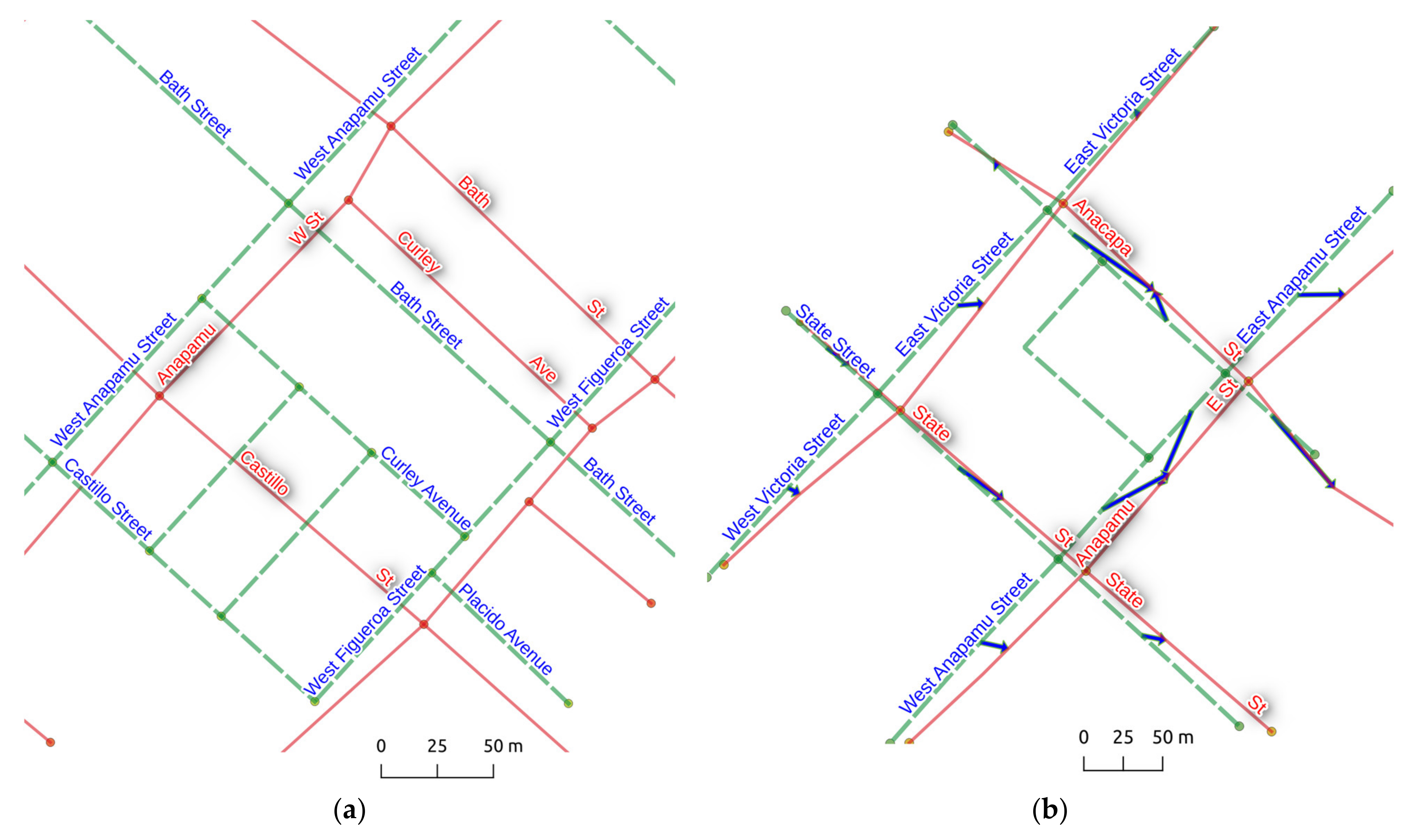
Figure 1. Conflation issues with OpenStreetMap (green) and TIGER (red) networks in downtown Santa Barbara, CA. Blue arrows represent matches. (a) Spatial offsets defeat spatial joins; (b) full and partial matches in a street block.
Ijgi 11 00375 g001
Figure 2. Transitive assignments: (a) transitive assignments in fc-bimatching; (b) removing transitive assignments with u-bimatching.
Ijgi 11 00375 g002
Figure 3. Test data at six sites in Santa Barbara County, CA, from OSM (green) and TIGER (red), respectively.
Ijgi 11 00375 g003
Figure 4. Precision rates of optimized conflation models for the Santa Barbara dataset (OSM vs. TIGER). (af) Results for sites #1 through #6.
Ijgi 11 00375 g004aIjgi 11 00375 g004b
Figure 5. Recall rates of optimized conflation models for the Santa Barbara dataset (OSM vs. TIGER). (af) Results for sites #1 through #6.
Ijgi 11 00375 g005
Figure 6. F-score of optimized conflation models for the Santa Barbara dataset (OSM vs. TIGER). (af) Results for sites #1 through #6.
Ijgi 11 00375 g006aIjgi 11 00375 g006b
Figure 7. Percentage of full matches produced by tested optimized conflation models for the Santa Barbara dataset (OSM vs. TIGER). (af) Results for sites #1 through #6.
Ijgi 11 00375 g007aIjgi 11 00375 g007b
Publisher’s Note: MDPI stays neutral with regard to jurisdictional claims in published maps and institutional affiliations.