Exploring the Impact of Floating Population with Different Household Registration on Theft

Abstract

The floating population is frequently treated as a homogeneous whole to explore its impact on crime in numerous crime studies in China. However, there are different compositions within the floating population and significant differences in the effects on crime. In this study, the floating population was divided into three types based on household registration (i.e., Hukou): the floating population from other districts in the same city (FPFOD), the floating population from other cities in the same province (FPFOC) and the floating population from other provinces (FPFOP). The Moran index was used to analyze their spatial distribution patterns and aggregation, respectively, and several negative binomial regression models were constructed to explore the influence of different types of floating populations on theft. The results show that the three types of floating populations are mainly distributed in different urban areas, implying differences in their impact on theft. Among them, the proportion of the FPFOD shows insignificant negative correlation on theft, while the proportion of the FPFOC and the FPFOP present a significant positive correlation. Meanwhile, the proportion of the FPFOP creates a stronger effect on theft than the proportion of entire floating population. Overall, the model performs best when variables of the proportion of the FPFOC and the FPFOP are included. The research conclusions can provide a meaningful reference for precisely measuring the floating population in crime research.

1. Introduction

The floating population refers to people who leave their domicile for work, study, etc., and go to live and work in a different place [1,2]. In the census, a population whose current place of residence is not in the same township or street as their registered place of residence is considered as the floating population. According to the 2017 China Floating Population Development Report [3,4], the total floating population in China was 245 million in 2016, which still accounted for 17.72% of the national population, although the total number decreased compared with previous years. The large size of the floating population plays a significant role in the city, because the economic, social as well as cultural development of the city cannot be achieved without the efforts of the floating population [5,6,7,8]. Depending on the location of registration, the floating population is further subdivided into three categories in the census: the floating population from other districts in the same city (FPFOD), the floating population from other cities in the same province (FPFOC) and the floating population from other provinces (FPFOP) [9].

With the advancement of globalization and urbanization, the living conditions, physical and mental health status and community integration of floating populations in cities have received increasing attention, and how to protect the rights and interests of floating populations and facilitate their better adaptation to local life has been on the working agenda of many cities. As such, crime problems associated with floating populations have also attracted extensive attention. On the one hand, frequent crime will affect the sense of happiness and security of floating populations living in the community. On the other hand, frequent crime leads to local residents considering “crime is brought by the floating population”, which will lead to stigmatization of the floating population and other phenomena. In fact, the debate has never stopped on the issue of floating populations and crime [10]. Some argue that floating populations bring crime [11,12], while others think that the relationship between floating populations and crime is not strong [13,14]. Therefore, what is the relationship between the proportion of the floating population in the community and the frequency of crime occurrence? Does the increase in the floating population in the community really have an impact on crime? Intrigued by these questions, we decided to take a look.

2. Literature Review

At present, studies on floating populations have generally focused on the fields of medical services [15,16,17], sociology [18,19] and geography [4,20,21,22,23,24,25,26,27,28,29]. Medical science links the conditions related to floating populations to the occurrence of certain types of diseases; sociology studies the social behavior, social forms and social organization of floating populations; geography studies mainly include the identification and analysis of floating population clusters [4,26,28], the spatial distribution of floating populations and the influencing factors [22,24,25], and the origin and migration direction of floating populations [20,23].

Among the relevant studies in geography, scholars have further explored the differences between floating populations with different household registration. In terms of mobility direction, local residents, the FPFOC and the FPFOP are attracted to third-tier, second-tier and first-tier cities, respectively [30]. When it comes to the spatial distribution of the floating population, the FPFOD usually tends to choose to live in the urban center with higher development. In contrast, the FPFOC and the FPFOP prefer to live in the city’s peripheral areas [31]. The FPFOD settlement area has various supporting facilities and better living conditions. Still, the living environment in the FPFOC and the FPFOP settlements are not as good as that of the FPFOD, and the infrastructure has not yet been improved. Concerning settlement intentions, the FPFOC tends to settle permanently in the inflow area, while the FPFOP prefers short-term and long-term stays [32].

The mobility of residents has long produced a classic body of literature regarding its impact on crime. Many scholars have included floating populations in crime research and explored the correlation between floating populations and different types of crimes. Mao and Ding [33] treated the foreign inflow population as one of the urban environmental factors and studied its influence on the number of robberies and snatching cases; Wang Yang et al. [34] included the proportion of the foreign inflow population in the construction of a comprehensive evaluation system for the risk of financial crimes. In recent years, many scholars have found that different floating population incomes, living environments, cultural backgrounds and education levels vary significantly. There are considerable differences between different types of floating populations. A study by Shi and Wu [35] showed that the increase in the overall size of the floating population does not lead to a rise in the crime rate, and the floating population’s type of work, residence and origin is highly correlated with the crime rate. Therefore, distinguishing the floating population according to different population characteristics is the work that needs to be performed in the detailed study of crime associated with the floating population. Lin Liu et al. [36] divided floating burglary offenders into four age groups. They found that neighborhoods with high residential instability attract more mobile adolescent floating burglary offenders, while socially disordered communities have more potent adult floating burglary offenders. Zhao et al. [37] divided criminals’ household registration into Changchun city center, non-Changchun city center in Jilin province and other provinces, finding that “local” perpetrators with domicile in Changchun city center were more familiar with the local area and traveled more widely to commit crimes. Chen et al. [21] divided the floating population into the floating population from other provinces and the floating population from the same province as ZG city and explored the influence of both on the number of burglaries.

3. Research Design

Based on the existing literature, this paper puts forward research questions. On the basis of the research questions, we constructed the conceptual framework [38,39,40], found the appropriate research area, researched data and researched methods to carry out the research.

3.1. Research Question

Several of the aforementioned studies are rich in content. Still, fewer have addressed the relationship between the floating population whose household registration is in the local city and crimes, and few have compared the differences in the impact of the floating population with different household registration on theft. Therefore, this study takes the community as the research unit, and subdivides the floating population into the FPFOD the FPFOC and the FPFOP. Further negative binomial regression models will be used to determine the differences in the impact of each type of floating population on theft. Based on this topic, we also want to discuss the spatial distribution and differences in different floating populations here, on the one hand, to better understand the basic situation of floating populations in communities, and on the other hand, to provide a partial basis for explaining the differences in the impact of different floating populations on community crimes. This paper mainly uses the method of Local Moran’s I to explore the difference in spatial distribution. As a result, the following two research questions are proposed in this paper.

Question 1: Are there any differences in the spatial distribution of the floating population with different household registration?

Question 2: What is the impact of the floating population with different household registration on theft?

By considering these two questions, this paper tries to explore the relationship between the floating population with different household registration and theft, refine the research on the floating population in crime geography, provide relevant cases for the application of the negative binomial regression method in crime geography, and also provide reference ideas for management agencies in community management and security.

3.2. Conceptual Framework

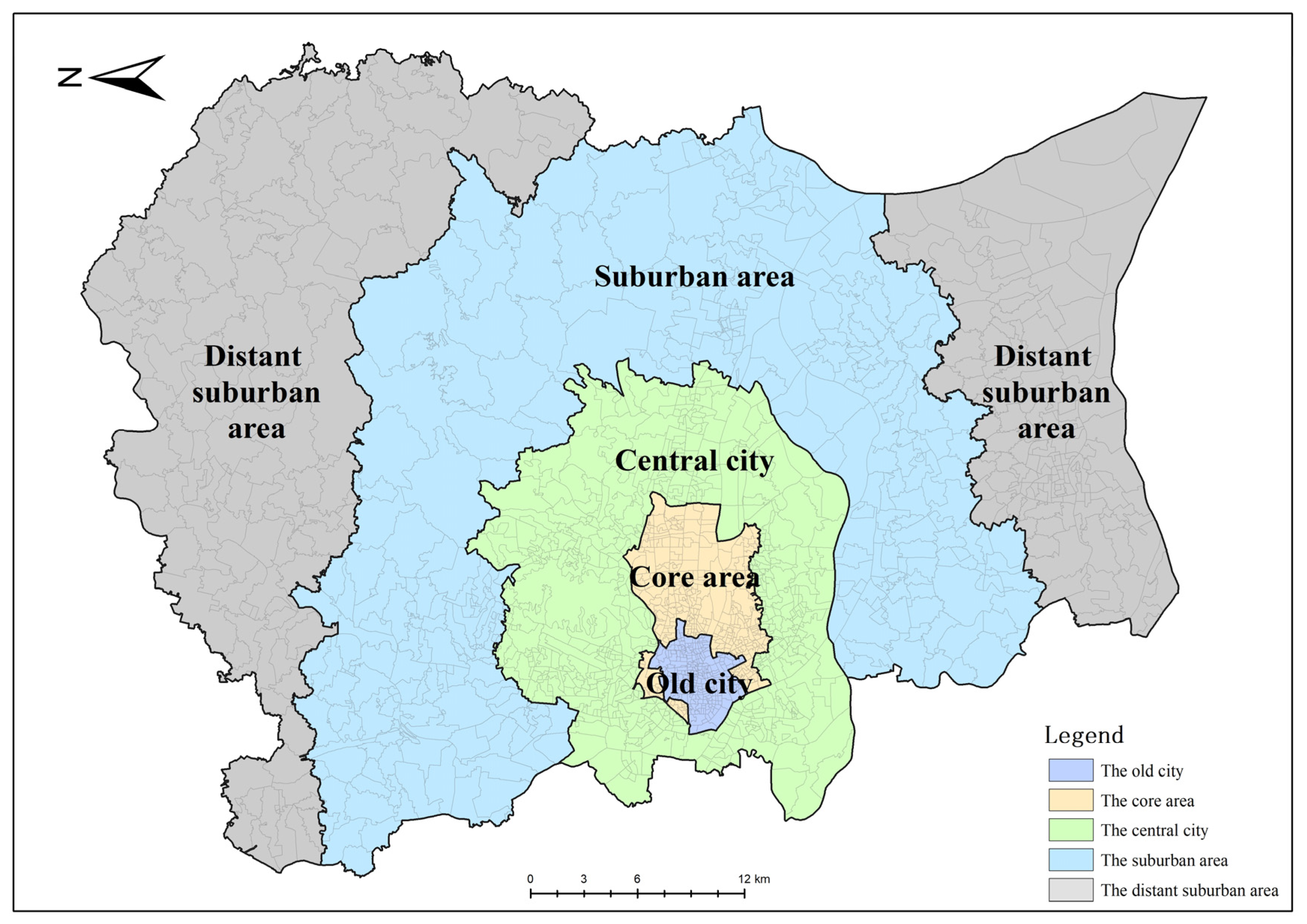
Some classical theories in the field of criminal geography have been used up to now, including social disorganization theory [41,42,43,44,45,46] and crime pattern theory [37,47,48,49,50]. Our conceptual framework is mainly based on these two theories.

Social disorganization theory emphasizes the effect of poverty, residential mobility and racial/ethnic heterogeneity on the informal control of communities [42,44]. When poverty, residential mobility or racial/ethnic heterogeneity increases in a community, the community’s informal control is weakened and all types of criminal behavior are more likely to occur there [42,51,52]. It uses the proportion of low-rent households as a measure of poverty. Generally speaking, if people have a low income, they will choose a house with a relatively low rent to save their living expenses. Meanwhile, the proportion of the floating population is used to represent residential mobility and racial/ethnic heterogeneity. The floating population generally does not have fixed real estate in the local city and mainly rents houses [53], so it is easier to relocate than the local residents. At the same time, the floating population will also have specific differences from the residents in terms of accent, eating habits and regional cognition, so their integration into the community will be hindered [54]. When the proportion of the floating population in the community increases, the residential mobility and racial/ethnic heterogeneity of the community will increase. Due to the differences among different floating populations, their proportion in the community will also have different impacts on residential mobility and racial/ethnic heterogeneity. For example, differences in accents, eating habits and regional perceptions between FPFOD and local residents were small, while differences between FPFOP and local residents were large. They have different effects on community heterogeneity. Therefore, this paper uses the proportion of the FPFOD, the FPFOC, the FPFOP and entire floating population to more specifically characterize the residential mobility and racial/ethnic heterogeneity of communities.

At the same time, social disorganization theory also emphasizes the influence of concentrated disadvantage and social control on community crime [45,46]. When the degree of concentrated disadvantage is high in a community, this community is easier to suffer from crime. Proportion of the population with secondary and lower education levels as well as the youth population are used here to indicate the degree of concentrated disadvantage. It is generally believed that the increase in the proportion of the population with secondary and lower education levels and the proportion of the youth population will increase the degree of concentrated disadvantage in a community. In addition, when the social control ability is strong, criminals will not easily commit crimes in the community, so it will reduce the risk of crime there. More common symbols of social control include police, security personnel and patrol officers. Therefore, the number of police stations is selected as a measure of social control. The more police stations there are in a community, the better it is to deter and catch criminals, thus improving the community’s ability of social control.

Crime pattern theory [47] believes that the choice of crime sites is not random, but has obvious rules. It can be seen that criminals usually choose places they are familiar with, such as workplace, residence, entertainment places, public transportation stations and the routes connecting them as crime sites. The reason is that they can be more sure of committing crimes in the familiar space than in some completely unfamiliar location. These locations are known as “crime generators” and “crime attractors” [48,49,50] because of the frequency of crime. It is using shopping centers [55], parks, squares, banks, hospitals, schools, hotels [56] and restaurants to represent them.

To sum up, the conceptual framework of this paper can be obtained (Figure 1).

3.3. Research Area

The area studied in this paper is the main urban area of ZG city, which includes seven administrative districts. These municipal districts have more frequent economic activities, relatively better social and cultural conditions, and are areas with large population concentrations. ZG city is located in the south of China, bordering the South China Sea. Thanks to its particular geographical location and the policy of reform and opening up, ZG city has experienced remarkable economic development in recent years. In 2019, the gross domestic product of ZG city exceeded 20,000 billion yuan, with a year-on-year growth of 6.8%. Economic development has led to social, cultural and transportation progress. At the end of 2019, the permanent population of ZG city exceeded 9.5 million, of which nearly 80% is a non-agricultural population [57].

ZG’s high level of economic development and sophisticated transportation facilities have attracted many floating populations to live, work and do business in the city. In the past decade, ZG has been one of the major inflow areas for the domestic floating population, which reached 6,255,800 in 2010, accounting for 39.84% of the city’s total population. Compared to 2000, the floating population in ZG city increased by 19,847,700 people, with a growth rate of 41.92% [58]. The rapid growth of the floating population complicates the demographic structure of society, which in turn may breed crime problems. Therefore, it is highly feasible and necessary to conduct a study on the floating population in ZG city.

The development level of municipal districts within the main urban area is generally higher, but there are still some differences between different regions within it. Therefore, according to the practice of Wang Yang, Zhang Hong’ou and Wu Kangmin [34,59,60,61], this study further divides the main urban areas into old, core, central, suburban and distant suburban areas based on available literatures and the actual situation (Figure 2). The city’s infrastructure, such as transportation and medical care, gradually improves from the distant suburbs to the core area. Economic, livelihood and technological development increase progressively, while land rent and housing purchase costs also increase.

3.4. Data

The data used in this study consisted of theft data, floating population, socio-economic variables in the control variables, and Point of Interest (POI). The names, extreme values, means and S.D. of these data are shown in

Table 1. Descriptive statistics of variables.

Types of Variables	Attributes	Minimum	Maximum	Mean	S.D.
Dependent variable	Number of thefts in the security category	0.00	478.00	31.41	42.44
Independent variables	Proportion of the FPFOD (%)	0.00	0.93	0.13	0.13
	Proportion of the FPFOC (%)	0.00	0.76	0.13	0.10
	Proportion of the FPFOP (%)	0.00	0.88	0.20	0.17
	Proportion of the entire floating population (%)	0.00	0.99	0.47	0.24
Control variables	Number of residents	8.00	51,429.00	5733.73	4568.98
	Proportion of the youth population (%)	0.00	0.65	0.12	0.04
	Portion of the population with secondary and lower education levels (%)	0.07	1.00	0.78	0.18
	Proportion of households with a monthly rent of less than 500 yuan (%)	0.00	1.00	0.55	0.36
	Number of police stations	0.00	11.00	1.23	1.58
	Number of shopping centers	0.00	26.00	1.67	2.79
	Number of parks and squares	0.00	16.00	0.36	0.92
	Number of banks	0.00	19.00	0.76	1.46
	Number of hospitals	0.00	18.00	0.88	1.58
	Number of schools	0.00	92.00	1.84	4.95
	Number of hotels	0.00	19.00	1.74	2.57
	Number of restaurants	0.00	90.00	7.98	10.35

.

The dependent variable used in this study is the number of thefts in the security category in 2018. This These include attributes such as the type of case, the street where it is located, the time of occurrence, and the geographical location. Compared to robbery, assault and other types of crime, the security category of theft incidents is more numerous and more widely distributed in ZG city. The relevant conclusions drawn from this category of crimes as research objects have greater generality for crime prevention and control.

The floating population data are from the sixth national population census. As official data open to the whole society, the census data have low accessibility and high credibility. They, therefore, have been applied by many scholars to the study of crime geography [62]. The census data contain each community’s information on the area, the size of the FPFOD, the FPFOC, the FPFOP and permanent residents in ZG city. Meanwhile, we can obtain the total size of floating populations by adding up the size of floating populations of the three types in the community.

We included control variables in the model. These variables include community socio-economic variables and the POI. Among them, the socio-economic variables are derived from the 6th census data. They contain four variables, including the total number of residents in the community, the proportion of the youth population, the proportion of the population with secondary and lower education levels, and the proportion of households with a monthly rent less than 500 yuan. The total number of residents is the sum of the permanent and floating populations [63]. The youth population is defined as those in the community between the ages of 6 and 18. The proportion of people with an education level of high school and below can indicate the low literacy level of the community [64]. The proportion of households whose monthly rent is less than 500 yuan reflects the families with a relatively poor living environment and low living standards.

The POI data were obtained from the 2016 “Daodaotong” navigation electronic map, including police stations, shopping centers, parks, squares, banks, hospitals, schools, hotels and restaurants. These variables have been widely used in related studies [43,65,66,67,68,69,70]. As mentioned above, the police stations in these POIs represent the social control of the community, while others represent “crime generators” and “crime attractors”.

3.5. Research Method

With the support of the three types of data mentioned above, this study uses two main research methods, Local Moran’s I and the negative binomial regression model, to explore the distribution of the floating population, and its impact on theft.

3.5.1. Local Moran’s I

The Local Moran’s I [71] reflect the spatial correlation between one of the regional units and the surrounding restricted units [72]. Our research used the Local Moran’s I to show the aggregation of the floating population. Considering the spatial differences among communities, Geographical distance spatial weight matrix [73] is selected for analysis in this paper. For the i-th regional unit, the Local Moran’s I is calculated as follows:

$$I_i=\frac{Z_i}{S^2}{{\displaystyle \sum }}_{j\ne 1}^n{w}_{ij}{Z}_j$$

(1)

where $Z_i=y_i-\overline{y}$, $Z_j=y_j-\overline{y}$, $S^2=\frac{1}{n}{\displaystyle \sum }{\left(y_i-\overline{y}\right)}^2$, $w_{ij}$ is the spatial weight value, n is the total number of all regions in the study area, and $I_i$ represents the Local Moran’s I of the i-th region. According to the significance of $I_i$, whether it is a positive or negative number, and whether z is greater than 0, the i-th region can be divided into the “high–high clustering region”, the “high–low clustering region”, the “low–high clustering region” and the “low–low clustering region”. Specifically, if a community has a high–low floating population ratio and the surrounding communities have a similar situation, we call it the “high–high clustering region” or the “low–low clustering region”; if a community has a high percentage of migrants and the surrounding community has a low percentage of migrants, or if that community has a low percentage of migrants and the surrounding community has a high percentage of the floating population, we call it the “high–low clustering region” or the “low–high clustering region” [74].

3.5.2. Negative Binominal Regression

In previous studies [75], a negative binomial regression model is generally used to explore the relationship between the dependent and independent variables. Multiple linear regression requires the dependent variable to conform to a normal distribution, while negative binomial regression is suitable for cases where the dependent variable is excessively discrete. In this paper, the dependent variable (the number of theft crimes) has a mean μ = 31.413 and variance σ² = 1801.324. Its variance is much larger than its mean and presents a discrete state, which does not meet the requirements of normal distribution, so it is more suitable to use negative binomial regression. The equation of the negative binomial regression is as follows.

$$ln\left(y\right)=I+{\beta }_1{x}_1+{\beta }_2{x}_2+\dots +{\beta }_n{x}_n$$

(2)

where I is the intercept, $x_1, x_2,\dots ,x_n$ are the independent variables, and ${\beta }_1$, ${\beta }_2$, …, ${\beta }_n$ are the coefficients of the independent variables.

In this paper, the Variance Inflation Factor (VIF) is used to test for the multicollinearity of variables [76]. If the Variance Inflation Factors (VIFs) are too large, this indicates that the cointegration between the factors is too strong and thus will have a bad effect on the final results of the model. The model needs to be readjusted if the VIF is too high. The following formula calculates the VIF.

$$\mathrm{VIF}=\frac{1}{1-R^2}$$

(3)

The Akaike Information Criterion (AIC) [77] and the Bayesian Information Criterion (BIC) [78] are suitable criteria to measure the goodness of fit between statistical models [79].

4. Results

Spatial autocorrelation analysis and negative binomial regression were used to obtain the distribution of the floating population, the aggregation, and the exploratory model results. Further analysis of the results can answer the two research questions of this paper.

4.1. Results of Spatial Analysis

The spatial distribution of the entire floating population is extensive, which is found in most of the communities (Figure 3a). Compared with that, the agglomeration points of the FPFOD are scattered, and the distribution areas are discontinuous. As shown in Figure 3b, the FPFOD is concentrated in the core and central urban regions. At the same time, the suburban and distant suburban areas also have a partial distribution of the floating population on the right side. The communities with a high proportion of the FPFOC are connected into patches, and most of them are located in the central city and suburban areas (Figure 3c).

In addition, Figure 3d shows that communities with a high proportion of the FPFOP are the most widely distributed and connected, with contiguous areas spreading from the central city to the near and distant suburban areas. We can conclude that there are some differences in the spatial distribution of the floating population by household registration. As the floating population increases across administrative divisions, areas with a higher proportion of distribution gradually move from core areas to distant suburban areas.

The Local Moran’s I was calculated separately for the floating population of different household registration and the entire floating population. At the macro-level (Figure 4a), the “high–high” agglomeration of the entire floating population is distributed contiguously at the junction of the central city and the suburbs. In contrast, the “low–low” agglomeration is mainly spread in the old city, most of the core area, and the southwest and northeast corners of the distant suburbs. The FPFOD (Figure 4b) forms a ring around the old city and the core area with a combination of “high–high” and “low–high” clusters. At the same time, the FPFOD is less distributed in the southwest and northeast corners of the suburban and distant suburban areas, forming a large “low–low” agglomeration area. The FPFOC (Figure 4c) is similar to the entire floating population, but the “low–low” clusters in the northwest and northeast corners of the far suburbs are more dispersed.

Compared to the FPFOC and the entire floating population, the FPFOP (Figure 4d) also shows a wide presence of “low–low” agglomerations in old cities and core areas. However, the number and scope of “low–low” agglomerations are smaller in the distant suburbs, while the number of “high–high” agglomerations is larger and more widely distributed. As the floating population increases across administrative divisions, the “low–low” agglomerations cluster from distant suburbs to old cities and core areas. The “high–high” agglomerations cluster from old cities and core areas to distant suburbs.

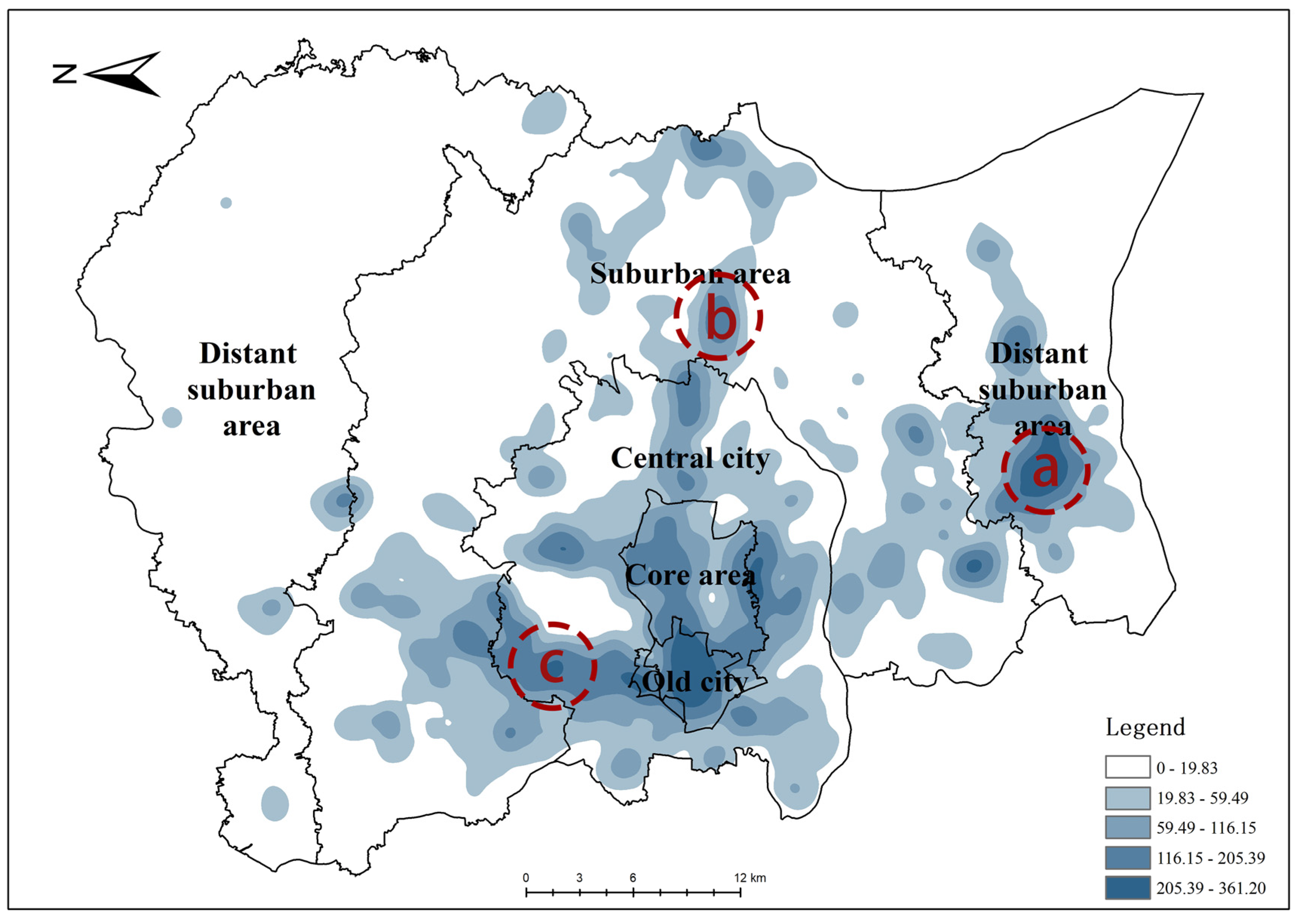
4.2. Spatial Distribution of Theft

Figure 5 shows the spatial distribution of theft crime. From the figure, it can be learned that the highest concentration of theft crime is in the center of the old city and the center of the distant eastern suburbs. In addition, a concentrated contiguous crime hotspot area is formed along with the old city-core area-central city, while some high-crime areas also exist in the near and distant suburban areas. Specifically, district a is the center of the distant suburban area, which has been the location of the county and district governments since the founding of the country and is currently crossed by provincial roads and subway lines. District b is near the river and has long been a commercial boom in the suburban area. With the opening of the subway station, more and more famous stores have settled here and formed a rather distinctive zigzag commercial area. District c is located in the community of the central city. This community having more residents and rich folk culture is surrounded by scenic spots such as parks, temples as well as water parks, and has the airport highway passing by on one side. Overall, most of the high incidences of theft are in areas with dense populations, convenient transportation and frequent economic activities.

4.3. Results of Regression Models

We constructed eight negative binomial regression models, adding a single variable and multiple variables based on the control variables, respectively, to express the relationship between the independent variable and theft and compare each model’s goodness of fit. Statistics and calculations show that the VIFs of all variables in all models are less than 2.3 [48], indicating no apparent collinearity between variables. It is suitable for negative binomial regression models.

4.3.1. Model Results of Adding a Single Floating Population Type

Model 1 was put into both the control variable and the entire floating population proportion to verify the effect of the entire floating population proportion on theft and its significance. Based on model 1, the variable of the entire floating population proportion was replaced by variables of the proportion of the FPFOD, the FPFOC, the FPFOP, respectively. Models 2, 3 and 4 were obtained to test their respective effects on theft.

The model results show that the number of residents, the proportion of the population with a high school education or less and the proportion of the household with a monthly rent of less than 500 yuan all show a significant positive correlation with theft. In contrast, the proportion of the youth population is positive but not significant. The shopping centers, parks, squares, banks, hospitals, hotels and restaurants positively affected theft, while the schools were negatively and insignificantly correlated. For the floating population variable, the relationship between the proportion of the FPFOD and theft showed a statistically significant negative correlation, while the proportion of the FPFOC and the FPFOP had a positive effect on theft.

The comparison between variables shows that the proportion of the FPFOP has the highest IRR value and has the greatest effect on the model, while the proportion of the FPFOC is the second and the proportion of the FPFOD is the lowest. By comparing between models, it can be found that model 4 has the lowest AIC and BIC (

Table 2. Results of Model 1–4.

Attributes	Model 1		Model 2		Model 3		Model 4
	β	IRR	β	IRR	β	IRR	β	IRR
Number of residents	<0.001 ***	1.000	<0.001 ***	1.000	<0.001 ***	1.000	<0.001 ***	1.000
Proportion of the youth population	0.378	1.459	0.103	1.109	0.175	1.191	1.047 *	2.849
Proportion of the population with secondary and lower education levels	0.483 **	1.620	0.463 **	1.590	0.565 ***	1.760	0.047	1.048
Proportion of households with a monthly rent of less than 500 yuan	0.186 **	1.205	0.157 *	1.170	0.180 *	1.198	0.106	1.112
Number of police stations	0.029 *	1.029	0.018	1.018	0.022	1.022	0.030 *	1.031
Number of shopping centers	0.055 ***	1.056	0.061 ***	1.063	0.061 ***	1.063	0.043 ***	1.044
Number of parks and squares	0.150 ***	1.162	0.145 ***	1.156	0.158 ***	1.171	0.138 ***	1.148
Number of banks	0.082 ***	1.086	0.067 ***	1.070	0.080 ***	1.083	0.081 ***	1.084
Number of hospitals	0.079 ***	1.082	0.064 ***	1.067	0.075 ***	1.078	0.071 ***	1.073
Number of schools	−0.005	0.995	−0.010	0.990	−0.010 *	0.990	−0.003	0.997
Number of hotels	0.041 ***	1.042	0.047 ***	1.048	0.040 ***	1.041	0.045 ***	1.046
Number of restaurants	0.028 ***	1.029	0.029 ***	1.030	0.028 ***	1.029	0.028 ***	1.028
Proportion of the FPFOD	-	-	−0.380 *	0.684	-	-	-	-
Proportion of the FPFOC	-	-	-	-	1.374 ***	3.952	-	-
Proportion of the FPFOP	-	-	-	-	-	-	1.454 ***	4.280
Proportion of the entire floating population	0.719 ***	2.052	-	-	-	-	-	-
_cons	1.461 ***		1.857 ***		1.553 ***		1.850 ***
lnalpha_cons	−0.568 ***		−0.535 ***		−0.555 ***		−0.590 ***
pseudo R~q	0.081		0.078		0.080		0.084
AIC	13,572.20		13,626.40		13,592.00		13,538.90
BIC	13,653.40		13,707.60		13,673.20		13,620.10

Note: ①*** Parameters are significant at the 0.001 confidence level. ** Parameters are significant at 0.05 confidence level. * Parameters are significant at the 0.01 confidence level; ②AIC and BIC show the effect of model fitting. If the values of AIC and BIC are smaller, the fitting effect of the model is better.

), followed by model 1. This indicates that the model works best when the proportion of the FPFOP is included and is better than the model consisting of the proportion of the entire floating population.

4.3.2. Model Results of Adding Multiple Floating Population Types

The influence of a single floating population variable on the model is limited. This study attempts to add more than one floating population variable on the basis of the control variable to explore the differences in the interpretation effects of single and multiple floating population variables on the model.

Table 3. Results of Model 5–8.

Attributes	Model 5		Model 6		Model 7		Model 8
	β	IRR	β	IRR	β	IRR	β	IRR
Number of residents	<0.001 ***	1.000	<0.001 ***	1.000	<0.001 ***	1.000	<0.001 ***	1.000
Proportion of the youth population	0.351	1.420	1.110 *	3.033	1.031	2.805	1.105 *	3.021
Proportion of the population with secondary and lower education levels	0.456 **	1.578	0.003	1.003	0.113	1.119	0.061	1.063
Proportion of households with a monthly rent of less than 500 yuan	0.154 *	1.167	0.094	1.099	0.114	1.120	0.100	1.105
Number of police stations	0.021	1.021	0.030 *	1.030	0.030 *	1.031	0.030 *	1.030
Number of shopping centers	0.060 ***	1.062	0.042 ***	1.043	0.045 ***	1.046	0.044 ***	1.045
Number of parks and squares	0.157 ***	1.169	0.137 ***	1.147	0.144 ***	1.154	0.143 ***	1.154
Number of banks	0.079 ***	1.083	0.080 ***	1.084	0.085 ***	1.089	0.084 ***	1.088
Number of hospitals	0.072 ***	1.075	0.069 ***	1.071	0.074 ***	1.076	0.072 ***	1.074
Number of schools	−0.011 *	0.989	−0.004	0.996	−0.004	0.996	−0.005	0.995
Number of hotels	0.041 ***	1.042	0.046 ***	1.047	0.043 ***	1.044	0.043 ***	1.044
Number of restaurants	0.028 ***	1.028	0.027 ***	1.028	0.027 ***	1.028	0.027 ***	1.028
Proportion of the FPFOD	−0.421 *	0.657	−0.200	0.816	-	-	−0.240	0.783
Proportion of the FPFOC	1.402 ***	4.062	-	-	0.605 *	1.830	0.634 **	1.885
Proportion of the FPFOP	-	-	1.438 ***	4.213	1.276 ***	3.583	1.249 ***	3.486
Proportion of the entire floating population	-	-	-	-	-	-	-	-
_cons	1.691 ***		1.916 ***		1.757 ***		1.832 ***
lnalpha_cons	−0.559 ***		−0.591 ***		−0.594 ***		−0.595 ***
pseudo R~q	0.080		0.084		0.084		0.084
AIC	13,588.90		13,539.70		13,534.30		13,534.50
BIC	13,675.40		13,626.20		13,620.80		13,626.40

Note: ①*** Parameters are significant at the 0.001 confidence level. ** Parameters are significant at 0.05 confidence level. * Parameters are significant at the 0.01 confidence level; ②AIC and BIC show the effect of model fitting. If the values of AIC and BIC are smaller, the fitting effect of the model is better.

shows the results of models 5 to 8, i.e., the effects of the proportional variables of the FPFOD, the FPFOC and the FPFOP when they are paired two by two or all put together in the model. From the results, the significance, positivity, negativity of the socio-economic and POI variables are generally consistent with the results of models 1–4. Meanwhile, the proportion of the FPFOD has always negatively influenced theft crime, even if its statistical significance has shown to be unstable. The statistical significance of the proportion of the FPFOC and the FPFOP is more stable than the proportion of the FPFOD, and both offer a positive correlation with theft. The comparison between the variables within the model shows that the IRR value of the proportion of the FPFOP is still the highest, and the proportion of the FPFOD is the lowest. Through the comparison between models, it can be found that model 7 has the lowest AIC and BIC (Table 3), and model 5 has the highest value (Table 3). The data show that the model with the proportion of the FPFOC and the FPFOP has the best effect among the four multivariate models. In contrast, the model with the proportion of the FPFOD and the FPFOC has the worst impact.

The model results presented above are consistent with the conclusions of previous studies. Residents of the community will become potential victims, and more criminal targets and objects may be provided to the offender. Scholars such as Newman, Oscar [80], and Andresen [81] believe that the greater the population density, the greater the possibility of contact between motivated criminals and potential victims, contributing to crime. The significance of this variable in the model validates this claim.

Numerous studies believe that improving residents’ educational level is conducive to suppressing crime [64,82]. In this paper, the proportion of the population with high school education and below is positively correlated with theft in multiple models, indicating that theft is more common in communities with lower education levels, which is in line with previous conclusions. According to social disorganization theory, the income of the residents with lower education level is generally lower, which will increase the poverty level of the community and reduce the level of informal control, thus leading to more crimes.

The proportion of households with rents below 500 yuan positively affected theft in several models, consistent with the findings of previous studies [66]. A disproportionately high percentage of low-rent tenants in a community indicates a high level of poverty among the residents of that community. Based on social disorganization theory, communities with higher poverty levels have less formal control and are easy targets for crime.

In routine activity theory, police stations play the role of supervisors and can act as a solid deterrent to offenders, effectively preventing and suppressing the occurrence of crime. Therefore, it is generally believed that the number of police stations negatively correlates with the crime rate. However, a diametrically opposite conclusion was obtained in the present study. This article speculates that, police stations are usually set up in densely populated areas with chaotic environments, often high-crime areas, to better deter delinquency and protect residents. Additionally, there is another explanation for this phenomenon, that is areas around police stations are more easily patrolled, so crime is more likely to be detected in areas with more police stations.

As mentioned above, shopping centers [65,83], park, squares [56,83], banks [56], hospitals, hotels [83,84] and restaurants [67] tend to gather large crowds of people, causing encounters between potential victims and motivated offenders and thus inducing crime. In this paper, we obtained similar findings to those of existing studies that the number of these POIs positively contributes to theft.

The differences in the impact of theft among the FPFOD, the FPFOC and the FPFOP are caused by the differences between the floating populations themselves. The FPFOD, although not currently living in their domicile, are still born and live in ZG city and have a very in-depth knowledge of the city’s customs, language as well as history, and their level of expertise and familiarity with ZG city is no less than that of local residents. As a result, they are primarily free of dilemmas in integrating into community life and interacting with local residents. From this perspective, communities with a high percentage of the FPFOD have sufficient cohesion, integration and informal control, which is conducive to reducing the probability of theft incidents.

The opposite is the FPFOC and the FPFOP. Their lack of knowledge of ZG city and language barriers can make it difficult for them to communicate with local residents. Therefore, communities with a high proportion of the FPFOC and the FPFOP have low cohesion and weak informal control and have a higher incidence of theft.

In terms of model effects, the model’s fit improved after using the proportion of the FPFOP instead of the proportion of the entire floating population. At the same time, if multiple categories of the floating population are included in the model, the effect of the model with variables of both proportion of the FPFOC and proportion of the FPFOP is better than other models. This is due to the more significant impact of the proportion of the FPFOC and the FPFOP on the model. In future related studies, if and when the floating population variable is involved, the variables of the FPFOC and the FPFOP can be used instead of the floating population to obtain better model effect.

Overall, the conclusions obtained in this study have some commonalities with current research findings. First, the proportion of the floating population does have a positive effect on theft, which is consistent with the results of scholars Chen and Qu [85] and Jin et al. [86]. Second, the relationship between the floating population and theft can be better explained by using social disorganization theory, crime pattern theory and routine activity theory, which is consistent with Kollamparambil et al. [87], Chen et al. [21], and Liu et al. [36]. Finally, this study confirms the findings of Shi and Wu [35] from the perspective of household registration, that the structure of the origin of the floating population is highly correlated with the crime rate.

5. Conclusions and Discussion

Based on the results, this paper conducted an empirical study on the spatial distribution of the floating population with different household registration and the differences in their impact on theft and obtained the following conclusions.

5.1. Conclusions

(1)

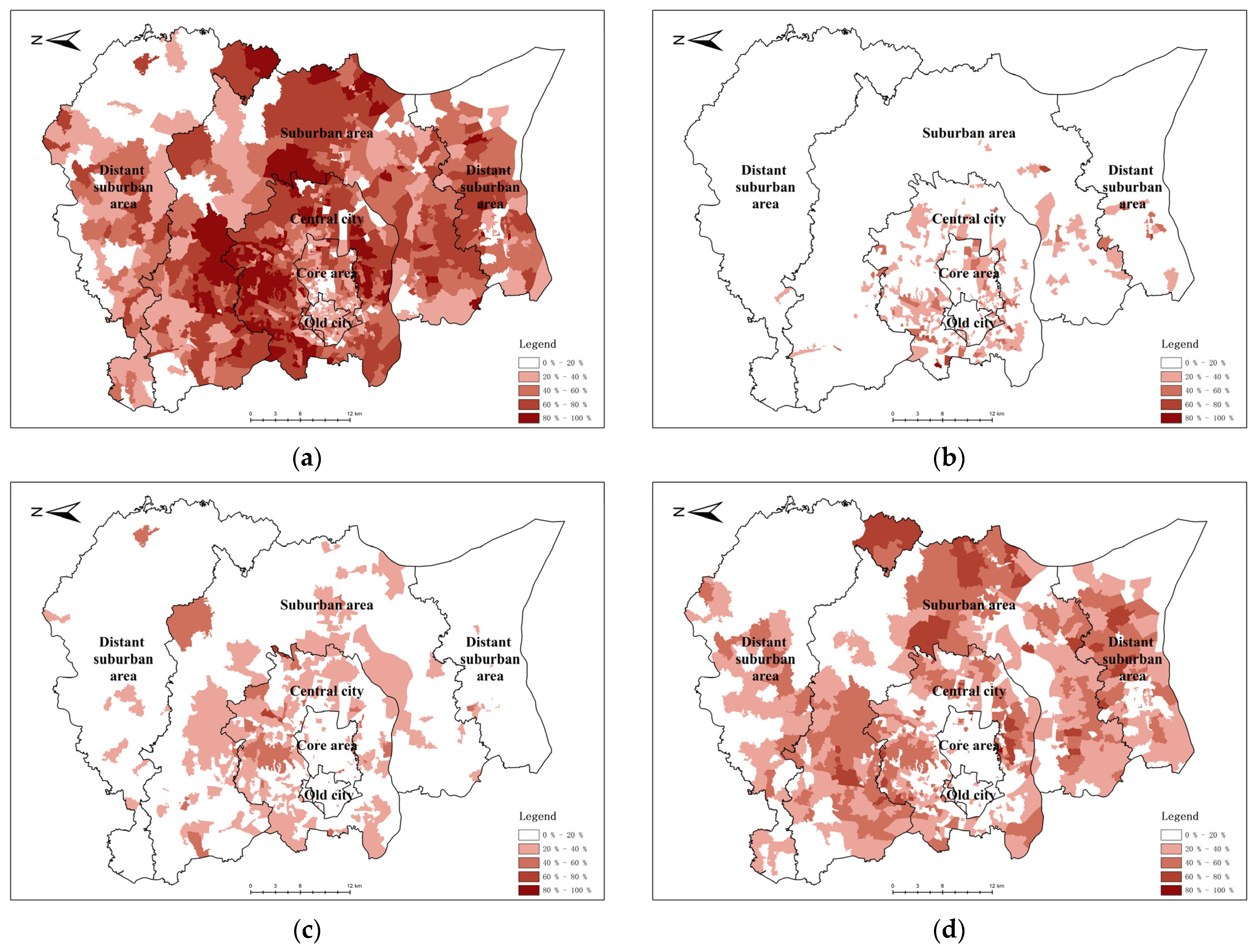
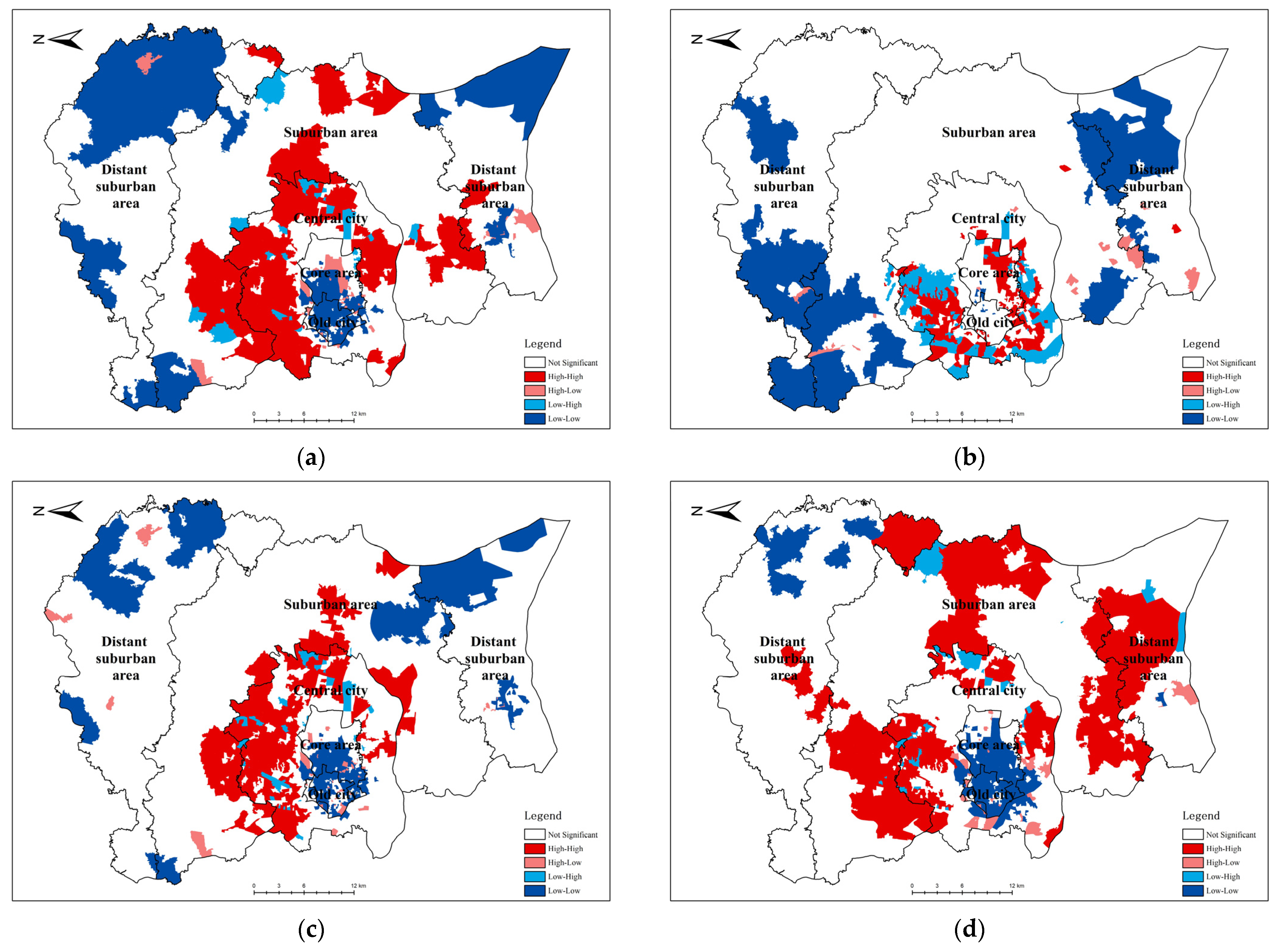
The spatial distribution of the floating population with different household registration varies. The FPFOD is concentrated in the downtown area. The FPFOC is concentrated in the suburban areas close to the city center and is closer to the distribution of the entire floating population. The FPFOP is mainly distributed in the immediate and distant suburban areas far from the city center. The spatial distribution is more dispersed than the other floating population. At the same time, with the increase in the floating population across administrative divisions, the “low–low” clusters are clustered from distant suburbs to old cities and core areas, and the “high–high” groups are clustered from old cities and core areas to distant suburbs.

(2)

The number of residents, the proportion of the population with a high school education or less, the proportion of the household with a monthly rent of less than 500 yuan, and POIs maintained a significant positive association with theft. The impact of the floating population on theft varies by household registration. The effect of the proportion of the FPFOD on theft was negative and, in some cases, insignificant. The proportion of the FPFOC and the FPFOP had a significant contribution to theft.

(3)

In terms of the model’s goodness of fit, the variables of the FPFOC and the FPFOP can be used instead of the floating population to obtain better model effect. In addition, if more than one category of the floating population is included in the model, the model works best when both the proportion of the FPFOC and the FPFOP are included.

5.2. Discussion

There are areas of this study that could be improved and refined.

Firstly, the population is constantly moving and migrating. Any type of floating population is no exception. Census data, however, are typically static, reflecting only the distribution of a population over a period of time, not how it has changed. Therefore, due to the lack of dynamic data [88], there is some uncertainty in the conclusion of this study.

Secondly, a number of readers may wonder what role floating population play in crime. Unfortunately, with the data currently available, our study cannot answer this question accurately. Further, the reason is, we have no statistics on the victims or perpetrators of theft, which makes it impossible to say who the perpetrators and victims are in a community.

In addition, the FPFOP actually comes from different provinces in China, with different local conditions and customs. However, we soon found that we could not further subdivide types of the FPFOP to further discuss the relationship between household registration and theft among the floating population because of lack of more detailed census data.

Finally, this paper mentions three classical theories of criminal geography and carries out subsequent analysis and research based on them. This is a common approach in the analysis of criminal geography. However, it can also lead to a series of problems [89]. For instance, structural factors are not included in theories’ explanations, which may lead to stigmatization of some population, or positive aspects of the floating population are not considered.

These shortcomings can be improved and refined in future studies. In the future research, there are several tasks that can be carried out: First, by combining the dynamic migration data of the floating population or the statistical data of the floating population for many years with the crime data of corresponding years, test whether the model results and conclusions in this study remain stable in a certain period of time. Second, obtain more detailed crime data, and judge the role of the floating population in community crime through empirical research. Third, this paper only divides the floating population into three categories. Follow-up studies can further subdivide the floating population according to their household registration attributes, and judge the relationship between the floating population from different provinces, cities or regions and crime. Fourth, combined with more theories and methods of non-criminal geography, follow-up studies can make a more in-depth qualitative or quantitative analysis of the floating population and community crime, and try to explain research questions of this paper from other perspectives.

The frequency of theft increases when informal controls in the community are weakened. Most of the existing studies have focused on the impact of the floating population on theft and less on further refinement of the floating population. The main innovations of this paper include the following. The FPFOD has been not been considered as often in previous studies and confirms the negative relationship between the FPFOD and theft. By comparing the AIC and BIC of each model, we find that the effect of the floating population with different household registration in the model shows an enormous difference. It can be found that the proportion of the FPFOP had the strongest effect on the increase in theft.

The findings of this paper can provide a theoretical basis for community management. When the proportion of the floating population in a community, especially the proportion of the FPFOC and the FPFOP, is high, the relevant personnel in charge of the community should help them integrate into the life of the community as soon as possible through various activities such as sports competitions, community preaching and seminars. In this way, the cohesiveness and informal control of the community can be improved, which will reduce the occurrence of crime.

References

1. Wu, R. Exploration of the meaning of floating population. Popul. Econ. 1990, 53–55. [Google Scholar]
2. Zhu, Z.; Zhu, R. Use and analysis of related concepts in urban floating population. Shanghai Urban Plan. Rev. 1997, 32–37. [Google Scholar]
3. Pan, Z. China’s Floating Population Development Report 2017: The Number of Floating Population in China Was 245 Million, and the Total Number of Floating Population Decreased for Two Consecutive Years. Available online: http://shanghai.xinmin.cn/xmsq/2017/11/10/31332612.html (accessed on 24 April 2022).
4. Qu, Y. Study on Crime Prevention and Control Mechanism of Floating Population Settlement Area. Ph.D. Thesis, People’s Public Security University of China, Beijing, China, 2018. [Google Scholar]
5. Du, J.; Xi, B. The Contribution of Labor-force flow to Economic Growth: An Options Perspective. South China Popul. 2010, 25, 52–58. [Google Scholar]
6. Ma, X.; Zhang, Y. Quantifying Economic Contribution of the Floating Population in the Cities. Popul. Res. 2004, 28, 63–67. [Google Scholar]
7. Ye, W.; Li, X.; Chen, Q. How lmmigrant Populations Affect City Entrepreneurship Activity: Mechanisms and Evidence. Econ. Res. J. 2018, 53, 157–170. [Google Scholar]
8. Du, X.; Chen, J. Empirical Analysis on Impacts of Migration with and without Hukou Change on China’s Provincial Economy. Popul. Res. 2010, 34, 77–88. [Google Scholar]
9. State Statistics Bureau. Population. Available online: http://www.stats.gov.cn/tjsj/zbjs/201912/t20191202_1713059.html (accessed on 12 October 2021).
10. Cheng, J.; Liu, J.; Wang, J. Domestic Immigration, Residential Status and Crime Rates. Sociol. Stud. 2016, 31, 218–241. [Google Scholar] [CrossRef]
11. Shan, Y. Cultural Conflict Theory on Crimes Committed by Migrant Workers. J. Natl. Prosec. Coll. 2009, 17, 115–122. [Google Scholar]
12. Zhou, S.; He, B. Trade Liberalization, Population Migration and Regional Crime Rate. J. Guizhou Univ. Financ. Econ. 2019, 1, 1–12. [Google Scholar]
13. Chen, Y. Construction and misdirection of Floating population in China. Popul. Dev. 2008, 14, 48–58. [Google Scholar]
14. Zhang, Y.; Liu, S.; Liu, L. Can We Attribute Increasing Criminal Rate to Enlarging Urban-rural lnequality in China? Econ. Resarch J. 2011, 46, 59–72. [Google Scholar]
15. Cai, X.; Yang, F.; Bian, Y. Gap analysis on hospitalized health service utilization in floating population covered by different medical insurances—Case study from Jiangsu Province, China. Int. J. Equity Health 2019, 18, 84. [Google Scholar] [CrossRef] [PubMed] [Green Version]
16. Su, L.; Sun, L.; Xu, L. Review on the prevalence, risk factors and disease Management of Hypertension among floating population in China during 1990–2016. Glob. Health Res. Policy 2018, 3, 24. [Google Scholar] [CrossRef] [PubMed] [Green Version]
17. Xu, C.; Wei, X.; Cui, J.; Wang, X.; Xu, D. Mixing in regional-structure model about the influence of floating population and optimal control about TB in Guangdong province of China. Int. J. Biomath 2017, 10, 1750106. [Google Scholar] [CrossRef]
18. Hao, P.; Tang, S. What keeps China’s floating population from moving? Chin. J. Sociol. 2018, 4, 1774829X–2057150X. [Google Scholar] [CrossRef]
19. Zhou, M.; Guo, W. Fertility intentions of having a second child among the floating population in China: Effects of socioeconomic factors and home ownership. Popul. Space Place 2020, 26, e2289. [Google Scholar] [CrossRef]
20. Ai, T.; Zhou, M.; Tian, J.; Ye, N. Origin–destination (OD) of the interprovincial floating population of China. J. Maps 2016, 12, 577–583. [Google Scholar] [CrossRef] [Green Version]
21. Chen, J.; Liu, L.; Zhou, S.; Xiao, L.; Jiang, C. Spatial Variation Relationship between Floating Population and Residential Burglary: A Case Study from ZG, China. Isprs. Int. J. Geo-Inf. 2017, 6, 246. [Google Scholar] [CrossRef] [Green Version]
22. Yuan, Y.; Xu, X.; Xue, D. Spatial distribution evolution and driving force of non—registered population of guangzhou metropolitan area in 1990–2000. Econ. Geogr. 2007, 6, 250–255. [Google Scholar]
23. Qiao, L.; Li, Y.; Liu, Y.; Yang, R. The spatio-temporal change of China’s net floating population at county scale from 2000 to 2010. Asia Pac. Viewp. 2016, 57, 365–378. [Google Scholar] [CrossRef]
24. Zhao, M.; Liu, S.; Qi, W. Exploring the differential impacts of urban transit system on the spatial distribution of local and floating population in Beijing. J. Geogr. Sci. 2017, 27, 731–751. [Google Scholar] [CrossRef] [Green Version]
25. Geng, H.; Shen, D. Spatial distribution and mechanism of migrant population in shanghai. City Plan. Rev. 2009, 33, 21–31. [Google Scholar]
26. Liu, H.; Gu, C. The Floating Population Concentration Areas in Beijing: Patterns, Structure and Functions. Sci. Geogr. Sin. 1999, 19, 497–503. [Google Scholar]
27. Liu, X.; Wang, M.; Cai, J.; He, M. An Analysis on the Spatial Structure of Non-Native Permanent Population of Beijing Metropolitan Area in 2000–2010. Urban Dev. Stud. 2013, 20, 86–93. [Google Scholar]
28. Wu, X. An Investigation into Marginal Community. City Plan. Rev. 2003, 27, 40–45. [Google Scholar]
29. Zhao, M.; Liu, S.; Qi, W. Comparison of foreign and domestic migrant communities: Characteristics and effects. City Plan. Rev. 2015, 39, 19–27. [Google Scholar]
30. Xue, C.; Wang, L.; Chang, F. Spatio-temporal Characteristics and Influencing Factors of Urban Floating Population in China. Areal Res. Dev. 2020, 39, 157–162. [Google Scholar]
31. Gao, X.; Ni, C. Residential Differentiation Characteristics and Influencing Factors of Migrants in Megacities—An Empirical Study of Nanjing. Xinjiang State Farms Econ. 2018, 5, 38–46. [Google Scholar]
32. Li, T.; Zhu, Y.; Lin, L.; Ke, W.; Xiao, B. The intentions of migrants with respect to duration of residence: Spatial variation and determinants. Acta Geogr. Sin. 2021, 76, 2978–2992. [Google Scholar]
33. Mao, Y.; Ding, J. Study On Spatial-Temporal Patterns Of Robbery And Snatch: A Case Study Of Pudong New Area, Shanghaia. Hum. Geogr. 2014, 29, 49–54. [Google Scholar]
34. Wang, Y.; Jin, L.; Zhang, H.; Wu, K.; Wang, Z.; Huang, G. Pattern and model of residential criminal risk based on social space in Guangzhou, China. Geogr. Res.-Aust. 2017, 36, 2465–2478. [Google Scholar]
35. Shi, J.; Wu, X. The Floating Population and China’s Crime Rate: An Empirical Study from 1997 to 2007. Res. Inst. Econ. 2010, 28, 1–20. [Google Scholar]
36. Liu, L.; Feng, J.; Ren, F.; Xiao, L. Examining the relationship between neighborhood environment and residential locations of juvenile and adult migrant burglars in China. Cities 2018, 82, 10–18. [Google Scholar] [CrossRef]
37. Zhao, Z.; Liu, D.; Xiao, J.; Wang, S. Spatial characteristics and influencing factors analysis of journey-to-crime based on crime pattern theory: A study of theft crime in Nanguan District, Changchun. Geogr. Res.-Aust 2021, 40, 885–899. [Google Scholar]
38. Shaw, M. Writing Good Software Engineering Research Paper. In Proceedings of the 25th International Conference on Software Engineering, Portland, OR, USA, 3–10 May 2003; IEEE Computer Society: Piscataway, NJ, USA, 2003; pp. 726–736. [Google Scholar]
39. Bryman, A. Integrating Quantitative and Qualitative Research: How Is It Done? Qual. Res. 2006, 6, 97–113. [Google Scholar] [CrossRef] [Green Version]
40. Bryman, A. Qualitative research on leadership: A critical but appreciative review. Leadersh. Q. 2004, 15, 729–769. [Google Scholar] [CrossRef]
41. Shaw, C.R.; Mckay, H.D. Juvenile Delinquency and Urban Areas. Soc. Serv. Rev. 1942, 35, 394. [Google Scholar] [CrossRef]
42. Roh, S.; Choo, T.M. Looking Inside Zone V: Testing Social Disorganization Theory in Suburban Areas. West. Criminol. Rev. 2008, 9, 1–16. [Google Scholar]
43. Willits, D.; Broidy, L.; Denman, K. Schools, Neighborhood Risk Factors, and Crime. Crime Delinq. 2013, 59, 292–315. [Google Scholar] [CrossRef]
44. Wong, S. Youth crime and family disruption in Canadian municipalities: An adaptation of Shaw and McKay’s social disorganization theory. Int. J. Law Crime Just. 2012, 40, 100–114. [Google Scholar] [CrossRef]
45. Gracia, E.; López-Quílez, A.; Marco, M.; Lladosa, S.; Lila, M. The Spatial Epidemiology of Intimate Partner Violence: Do Neighborhoods Matter? Am. J. Epidemiol. 2015, 182, 58–66. [Google Scholar] [CrossRef] [Green Version]
46. Sampson, R.J.; Raudenbush, S.W.; Earls, F. Neighborhoods and Violent Crime: A Multilevel Study of Collective Efficacy. Science 1997, 277, 918–924. [Google Scholar] [CrossRef] [PubMed]
47. Brantingham, P.; Brantingham, P. Crime pattern theory. Environ. Criminol. Crime Anal. 2013, 78–93. [Google Scholar] [CrossRef]
48. Bernasco, W.; Block, R. Robberies in Chicago: A Block-Level Analysis of the Influence of Crime Generators, Crime Attractors, and Offender Anchor Points. J. Res. Crime Delinq. 2011, 48, 33–57. [Google Scholar] [CrossRef]
49. Brantingham, P.; Brantingham, P. Criminality of place: Crime generators and crime attractors. Eur. J. Crim. Policy Res. 1995, 13, 5–26. [Google Scholar] [CrossRef]
50. Mahfoud, M.; Bernasco, W.; Bhulai, S.; Mei, R. Forecasting Spatio-Temporal Variation in Residential Burglary with the Integrated Laplace Approximation Framework: Effects of Crime Generators, Street Networks, and Prior Crimes. J. Quant. Criminol. 2020, 37, 835–862. [Google Scholar] [CrossRef]
51. Kornhauser, R.R. Social Sources of Delinquency; University of Chicago Press: Chicago, IL, USA, 1978. [Google Scholar]
52. Nielsen, A.L.; Hill, T.D.; French, M.T.; Hernandez, M.N. Racial/Ethnic Composition, Social Disorganization, and Offsite Alcohol Availability in San Diego County, California. Soc. Sci. Res. 2010, 39, 165–175. [Google Scholar] [CrossRef] [PubMed] [Green Version]
53. Jiang, L.; Pang, L.; Zhang, Z. Living Conditions of Floating Population in Urban China. Popul. Res. 2005, 21, 16–27. [Google Scholar] [CrossRef]
54. Zhao, H.; Liu, N. The Difference of Social lntegration of Floating Population from the Perspective of Family. Popul. Dev. 2018, 24, 2–13. [Google Scholar]
55. Browning, C.R.; Byron, R.A.; Calder, C.A.; Krivo, L.J.; Kwan, M.; Lee, J.; Peterson, R.D. Commercial Density, Residential Concentration, and Crime: Land Use Patterns and Violence in Neighborhood Context. J. Res. Crime Delinq. 2010, 47, 329–357. [Google Scholar] [CrossRef]
56. Jiang, X. Spatial Differentiation of the Impact of Urban Built Environment on Criminal Behavior. Ph.D. Thesis, Harbin Institute of Technology, Harbin, China, 2018. [Google Scholar]
57. Guangzhou Municipal Statistics Bureau; Guangzhou Survey Office of National Bureau of Statistics. Guangzhou Statistical Yearbook; China Statistics Press: Beijing, China, 2020; pp. 29–56. [Google Scholar]
58. Zhou, J.; Luo, X.; Xie, B. Spatial Distribution and Variation of Floating Population in Megacities—Case study of Bejing, Shanghai, Guangzhou and Wuhan. Urban Plan. Forum 2015, 6, 56–62. [Google Scholar]
59. Wang, Y.; Wu, K.; Zhang, H. The core influencing factors of housing rent difference in Guangzhou’s urban district. Acta Geogr. Sin. 2021, 76, 1924–1938. [Google Scholar]
60. Wang, Y.; Zhang, H.; Huang, G.; Zhang, Y.; Wu, K. Research on the Correlation and Spatial Variation between Urban Housing Characteristics and Social Space. Constr. Econ. 2017, 38, 100–104. [Google Scholar] [CrossRef]
61. Wang, Y.; Zhang, H.; Ye, Y.; Wu, Q.; Jin, L. Comprehensive Evaluation and Distribution Pattern of Social Space Quality in Guangzhou, China. Trop. Geogr. 2017, 37, 25–32. [Google Scholar] [CrossRef]
62. Du, F.; Liu, L.; Jiang, C.; Long, D.; Lan, M. Discerning the Effects of Rural to Urban Migrants on Burglaries in ZG City with Structural Equation Modeling. Sustainability 2019, 11, 561. [Google Scholar] [CrossRef] [Green Version]
63. Cabrera-Barona, P.F.; Jimenez, G.; Melo, P. Types of Crime, Poverty, Population Density and Presence of Police in the Metropolitan District of Quito. Int. J. Geo-Inf. 2019, 8, 558. [Google Scholar] [CrossRef] [Green Version]
64. Patrick, B. The heterogeneous effects of education on crime: Evidence from Danish administrative twin data. Labour. Econ. 2018, 52, S402094058X. [Google Scholar]
65. Hollinger, R.C.; Dabney, D. Motor Vehicle Theft at the Shopping Centre: An Application of the Routine Activities Approach. Secur. J. 1999, 12, 63–78. [Google Scholar] [CrossRef]
66. Liu, L.; Chen, D.; Xu, C.; Long, D.; Xiao, L.; Chen, X. Comparative study on the influencing factors of the distribution of near repeat cases and isolate cases of burglary. Sci. Geogr. Sin. 2021, 41, 1625–1633. [Google Scholar] [CrossRef]
67. Liu, L.; Liang, S.; Song, G. Explaining Street Contact Crime based on Dynamic Spatio-Temporal Distribution of Potential Targets. J. Geo-Inf. Sci. 2020, 22, 887–897. [Google Scholar]
68. Sebastian, B.; André, D. The place-based effects of police stations on crime: Evidence from station closures. J. Public Econ. 2022, 207, 104605. [Google Scholar]
69. Song, G.; Xiao, L.; Zhou, S.; Long, D.; Zhou, S.; Liu, K. lmpact of residents’ routine activities on the spatial-temporal pattern of theft from person. Acta Geogr. Sin. 2017, 72, 356–367. [Google Scholar]
70. Song, Y.; Huang, B.; Cai, J.; Chen, B. Dynamic assessments of population exposure to urban greenspace using multi-source big data. Sci. Total Environ. 2018, 634, 1315–1325. [Google Scholar] [CrossRef] [PubMed]
71. Anselin, L. Local Indicators of Spatial Association—LISA. Geogr. Anal. 1995, 27, 93–115. [Google Scholar] [CrossRef]
72. Bone, C.; Wulder, M.A.; White, J.C.; Robertson, C.; Nelson, T.A. A GIS-based risk rating of forest insect outbreaks using aerial overview surveys and the local Moran’s I statistic. Appl. Geogr. 2013, 40, 161–170. [Google Scholar] [CrossRef]
73. Liu, X.; Qu, Y. Spatial Agglomeration of Chinese Cultural Product Exports and its Evolutionary Trends. J. Nanjing Univ. Aeronaut. Astronaut. (Soc. Sci.) 2022, 24, 43–50. [Google Scholar] [CrossRef]
74. Song, Y.; Chen, B.; Ho, H.C.; Kwan, M.; Liu, D.; Wang, F.; Wang, J.; Cai, J.; Li, X.; Xu, Y.; et al. Observed inequality in urban greenspace exposure in China. Environ. Int. 2021, 156, 106778. [Google Scholar] [CrossRef] [PubMed]
75. Ao, Z.; Wang, J.; Sun, B. Impact of air quality on public outings based on big data. Resour. Sci. 2020, 42, 1199–1209. [Google Scholar] [CrossRef]
76. Man, J.; Yang, W. Based on Multiple Collinearity Processing Method. Math. Theory Appl. 2010, 30, 105–109. [Google Scholar]
77. Tohre, O.; Hiroyuki, O. Non-Linear Time Series Model Identification by Akaike’s Information Criterion. IFAC Proc. Vol. 1977, 10, 83–91. [Google Scholar]
78. Wang, H.; Miller, D. Improved Parsimonious Topic Modeling Based on the Bayesian Information Criterion. Entropy-Switz 2020, 22, 326. [Google Scholar] [CrossRef] [Green Version]
79. Song, G.; Liu, L.; Bernasco, W.; Xiao, L.; Zhou, S.; Liao, W. Testing Indicators of Risk Populations for Theft from the Person across Space and Time: The Significance of Mobility and Outdoor Activity. Ann. Am. Assoc. Geogr. 2018, 108, 1370–1388. [Google Scholar] [CrossRef]
80. Newman, O. Defensible Space: Crime Prevention Through Urban Design. Ekistics 1973, 36, 325–332. [Google Scholar]
81. Andresen, M.A. Crime Measures and the Spatial Analysis of Criminal Activity. Brit. J. Criminol. 2006, 46, 258–285. [Google Scholar] [CrossRef]
82. Long, D.; Liu, L.; Feng, J.; Song, G.; He, Z.; Cao, J. Comparisons of the community environment effects on burglary and outdoor-theft: A case study of ZH peninsula in ZG city. Acta Geogr. Sin. 2017, 72, 341–355. [Google Scholar]
83. Sherman, L.W.; Gartin, P.R.; Buerger, M.E. Hot Spots Of Predatory Crime: Routine Activities And The Criminology Of Place. Criminology 2010, 27, 27–56. [Google Scholar] [CrossRef]
84. Twinam, T. Danger Zone: The Causal Effects of High-Density and Mixed-Use Development on Neighborhood Crime. Ssrn Electron. J. 2014. [Google Scholar] [CrossRef]
85. Chen, P.; Ju, K. Analysis on the Factors That Affect Burglary in Urban Residential Communities—An Empirical Study of Beijing. J. People’s Public Secur. Univ. China 2018, 34, 67–71. [Google Scholar]
86. Jin, C.; Li, S.; Zheng, Z. Research on the Spatial distribution of floating Population and crime problem—From the perspective of the correlation between floating population gathering area and crime hotspot. J. People’s Public Secur. Univ. China 2014, 30, 1–10. [Google Scholar]
87. Kollamparambil, U. Immigration, internal migration and crime in South Africa: A multi-level model analysis. Dev. Policy Rev. 2019, 37, 672–691. [Google Scholar] [CrossRef]
88. Song, Y.; Huang, B.; He, Q.; Chen, B.; Wei, J.; Mahmood, R. Dynamic assessment of PM 2.5 exposure and health risk using remote sensing and geo-spatial big data. Environ. Pollut. 2019, 253, 288–296. [Google Scholar] [CrossRef] [PubMed]
89. Yang, L. A review of Chicago Social School crime theory. Chin. Criminol. Rev. 2016, 106–112. [Google Scholar]
Figure 1. Schematic diagram of conceptual framework.
Ijgi 11 00443 g001
Figure 2. Schematic diagram of the regional division of the study area.
Ijgi 11 00443 g002
Figure 3. The spatial distribution of the floating population with different household registration. (a) The proportion of the entire floating population; (b) the proportion of the FPFOD; (c) the proportion of the FPFOC; (d) the proportion of the FPFOP.
Ijgi 11 00443 g003
Figure 4. Moran’s I index distribution diagram of the floating population with different household registration. (a) The entire floating population; (b) the FPFOD; (c) the FPFOC; (d) the FPFOP.
Ijgi 11 00443 g004
Figure 5. Schematic diagram of the spatial distribution of theft cases.
Ijgi 11 00443 g005