Article

A Lightweight Long-Term Vehicular Motion Prediction Method Leveraging Spatial Database and Kinematic Trajectory Data

1
Graduate School of Informatics, Nagoya University, Nagoya 464-8601, Japan
2
Institute of Innovation for Future Society, Nagoya University, Nagoya 464-8601, Japan
*
Author to whom correspondence should be addressed.
ISPRS Int. J. Geo-Inf. 2022, 11(9), 463; https://doi.org/10.3390/ijgi11090463
Submission received: 27 June 2022 / Revised: 11 August 2022 / Accepted: 25 August 2022 / Published: 29 August 2022

Abstract

:
Long-term vehicular motion prediction is a crucial function for both autonomous driving and advanced driver-assistant systems. However, due to the uncertainties of vehicle dynamics and complexities of surroundings, long-term motion prediction is never trivial work. As they combine effects of humans, vehicles and environments, kinematic trajectory data reflect several aspects of vehicles’ spatial behaviors. In this paper, we propose a novel method that leverages spatial database and kinematic trajectory data to achieve long-term vehicular motion prediction in a lightweight way. In our system, a spatial database system is initially embedded in an extended Kalman filter (EKF) framework. The spatial kinematic trajectory data are managed through the database and directly used in motion prediction; namely, weighted means are derived from the spatially retrieved kinematic data and used to update EKF predictions. The proposed method is validated in the real world. The experiments indicate that different weighting methods make a slight accuracy difference. Our method is not data-and-computation-consumed; its performance is acceptable in the limited data conditions and its prediction accuracy is improved as the size of used data sets increases; our method can predict in real time. The efficiency of an unscented Kalman filter (UKF) is compared with that of the EKF. The results show that the UKF can hardly meet real-time requirements.

1. Introduction

Advanced driver-assistant system (ADAS) and autonomous driving (AD) are important components of a safe traffic society. ADAS uses various sensor technologies to provide information, warnings and assistance to the driver to improve his/her ability to react to dangers on the road through a human–machine interface. Further, AD allows vehicles to drive safely without any human intervention based on underlying perception, planning, decision and control systems. There is a common and foundational purpose among ADAS and AD areas: safe driving. Long-term vehicular motion prediction (LVMP) is an important technology for safe driving [1] due to its ability to predict vehicle situations in advance; the upcoming risk can therefore be detected. However, LVMP is never trivial work due to uncertainties concerning vehicular dynamics and complexities of surroundings.
For decades, various methods have been proposed to explain vehicle motion evolution over a long time range [2]. There are five main genres in LVMP studies: (1) physical model-based methods that use explicit mathematical expressions to describe vehicle motion evolution, such as [3,4]; (2) trajectory-matching-based methods that map vehicles’ trajectories into typical motion patterns to achieve long-term motion prediction, such as [5]; (3) machine-learning-based methods that learn prediction models from historical data, such as [6,7,8,9]; (4) map-aided methods that leverage map data, particularly geometries of high-definition (HD) maps, to realize long-term motion prediction, such as [10]; (5) hybrid methods that make use of at least two of the above methods, such as [11].
These methods try to cope with the uncertainties and complexities in LVMP from different perspectives. However, each kind of method has pros and cons and some challenges remain. The physical model-based methods are straightforward and efficient; however, a vehicle is governed by not only physical laws but also a human being and traffic environments, for example, road conditions and traffic signals. Our previous work showed that a single physical model was not able to make a reliable long-term prediction [12]. Trajectory-matching- and machine-learning-based methods receive reasonable predictions due to utilizing huge volumes of pre-prepared historical data. They therefore are computationally expensive and data-consumed; the prediction accuracy is heavily dependent on the richness of collected historical data. Map-aided methods take into account both functionality and efficiency. With mass productions of HD maps, there have been some typical map-aided methods proposed in recent years, such as [10,11,13]. However, these lack reasonable bases to fuse static map data that are defined by map makers with dynamic vehicle motion. A forced combination of them will make the prediction converge to static map data/attributes and the dynamics of the vehicle will surely be lost, for example, their trajectory prediction will converge to the lane center line and the predicted velocity will converge to the fixed velocity attributes in maps.
A particular trajectory can be regarded as an outcome of interactions between a particular vehicle and driver under particular environments. As records of dynamic vehicle motions, vehicles’ spatial kinematic trajectory data, such as position, velocity, yaw, yaw rate and acceleration, in fact reflect vehicles’ spatial behaviors in several aspects; for example, a position near the right side of a lane indicates that the vehicle would turn right; velocities and accelerations along different road segments were reflections of driving styles in different spaces. In vehicle motion predictions that are full of uncertainties, this information is crucial for corrections of mathematical models’ predictions. In order to overcome the disadvantages of the mentioned genres in LVMP, this paper, in a novel contribution, leverages spatial kinematic trajectory data that are retrieved through spatial relations to predict long-term vehicle motions in a Kalman filter (KF) framework.
The main contributions of this paper are summarized below:
  • A novel personalized LVMP method based on spatial database and kinematic trajectory data is proposed. Different from existing historical data-based methods that learn knowledge from huge volumes of data, our method retrieves relevant information based on spatial relations through a well-organized spatial database. In addition, the neglected personal factors in the present methods, such as driver and vehicle information, are taken into account in this paper.
  • A spatial database system is initially embedded in a classical KF framework. This combination makes our system lightweight and the utilization of a spatial search makes our algorithm able to find the most spatially related data quickly.
  • Both accuracy and efficiency of algorithms are discussed in this paper.
The remainder of this paper is organized as follows. Some related work is reviewed in Section 2. Then an overview of our system is given in Section 3 and the methodology of this paper is presented in detail in Section 4. The experiments are discussed in Section 5. Future work is summarized in Section 6 and the paper is concluded in Section 7.

2. Related Work

Long-term vehicular motion prediction is an important research area among AD and ADAS. In [12], the constant turn rate and velocity (CTRV) and constant turn rate and acceleration (CTRA) models were directly used to predict vehicle motion in an open loop KF framework without any external information correction; the results show that a sole mathematical model was not suitable for LVMP. Although a stand-alone physical vehicle motion model cannot predict reliably, switching between different motion models in different scenes using a Dempster–Shafer reasoning system can produce an accomplished prediction [4]. However, to date, few studies have only used physical models to conduct LVMP due to some inevitable constant hypotheses of motion models being unreasonable in a long time range. A compensation is to fully consider the uncertainties in predictions, such as [14,15,16].
Using historical data to predict vehicle motion in a long time range is a popular and dominant methodology. An early study can be dated back to 2009 [5]; the authors proposed a long-term motion method that combined trajectory classification and a particle filter framework. This was a so-called trajectory-matching-based method; they used a quaternion-based rotationally invariant longest common subsequence metric to measure trajectory similarity. Speed and timing profiles were introduced as presentations of surrounding environments in [17], in which a particle filter was used to incorporate information of environments and motion models. However, the algorithm only predicted one-dimensional positions along routes.Artificial Intelligence (AI) is a powerful paradigm for traffic prediction [18]. The Gaussian process was used to learn parameters of vehicular trajectories in [19]; moreover, to take into account vehicles’ interactions, a dynamic Bayesian network was utilized in [20]. In [21,22,23], graph neural networks were employed to model complex interactions between vehicles and roadside infrastructures. Deep neural networks were also adopted to predict ego-vehicle paths using environment observation in [24]. Long Short-Term Memory (LSTM) networks are widely used in sequence tasks, such as traffic and trajectory predictions. In [7], an LSTM network was used to predict vehicle trajectories on highways. Spatial and temporal attention mechanisms were introduced into LSTM networks in [8,9]. A common drawback of the above methods is that they have to collect large amounts of historical data for training in advance, and their computing cost is much higher; in this paper, we call that data-and-computation-consumed (DCC). In addition, these methods treat trajectory data from different drivers and vehicles as the same, which is unreasonable. For example, it is not applicable to use trajectory data of the old drivers to predict a young driver’s vehicle motion; it is also improper to use a sports car’s velocity profile to predict the velocity of a school bus. Personal characteristics, such as the driver’s and his/her vehicle’s information, should be taken into account.
The commercialization of HD maps provides a new solution for LVMP and its feasibility has been validated in some studies. In [10], an extended Kalman filter (EKF) was adopted to update the prediction made by a kinematic bicycle model using information acquired from HD maps, such as position, heading, and velocity. In the paper, squared Mahalanobis distance was used to assign traffic lane as an access to the map data. Similarly, in [13], an EKF was utilized to incorporate a uniform acceleration motion model and velocity model that was built based on HD map and observed velocities. In [11], the authors proposed an uncertainty-aware stitching method that combined short-term trajectories predicted by learned models with long-term actor goals derived from associated lanes. The map-aided methods force combinations of dynamic vehicle motions with static map data, which causes dynamics to be lost in LVMP.
In this paper, a new LVMP method is proposed. A comparison between the proposed method and some typical studies that are selected from the above-mentioned five genres is presented in Table 1. We can find from the table that: (1) our method does not belong to the five genres; novelly, it is implemented in a KF framework incorporating a spatial database; different from previous methods that need to collect a huge volume of training data and learn prediction models based on the data, which is DCC, our method directly retrieves information based on spatial relationships in the prediction process. The training process is not needed. (2) Compared with the map-aided methods that lose vehicle dynamics in predictions, our method leverages the driver’s spatial kinematic trajectory data to predict vehicle motions. Our predictions will converge to the driver’s personal driving styles in different spaces and the dynamics will be maintained. (3) furthermore, our prediction is personalized; information concerning the driver and the vehicle is considered.

3. System Overview

The inspiration for proposed method is Tobler’s first law of geography: everything is related to everything else, but near things are more related to each other [25]. In our context, we suppose that in most cases vehicle behaviors are spatially correlated; for example, on a certain lane segment, vehicles always exhibit similar velocities, and when they approach an intersection or a bend, they have to slow down. Based on these intuitions, we further suppose that, in most cases, as vehicle behaviors’ representations, vehicular states are spatially correlated. This makes LVMP possible where and when spatial kinematic trajectory data are available. Our system is illustrated in Figure 1.
The core components of our system are listed below:
  • A UKF state estimator. In real-world studies, prior to motion prediction, a real-time vehicle state estimator is necessary to reduce sensor noises; in our system, an unscented Kalman filter (UKF) that cooperates with a CTRA model is adopted. The UKF fuses information from the CTRA model and onboard sensors to make a reliable real-time vehicle state estimate at 10 Hz.
  • A spatial database for kinematic trajectory data management. The spatial database that maintains kinematic trajectory data and HD maps is a crucial component. The kinematic trajectory data, which contain spatial information, are stored in the spatial database to leverage a quick spatial query to realize real-time LVMP. The kinematic data are linked to the HD maps to facilitate the spatial query.
  • The lightweight LVMP algorithm. The utilization of the spatial database and EKF makes our method lightweight. The quick spatial search functions of the database provide the most spatially related information to our algorithm and thus we do not need to learn knowledge from huge amounts of data. The efficient EKF ensures real-time data processing.
As illustrated in the figure, a current vehicle state estimate made by the UKF is sent to the LVMP algorithm as an initial state. Then the state evolves into the next instant according to a CTRV model. At the predicted position, the surrounding kinematic trajectory points are queried from the spatial database and the virtual measurements are calculated. Finally, the predictions are corrected by the EKF using the virtual measurements. This process is iterated 50 times to achieve 5 s LVMP.

4. Methodology

4.1. Vehicle State Estimation

In order to predict vehicle motion, it is necessary to derive a vehicle’s state at the current time, such as accurate position and velocity estimates. In this paper, a UKF [26] is adopted in real-time vehicle state estimation.
For the sake of brevity, we give only two key functions in state estimation in this section; namely the process and observation functions. The following CTRA model is selected as the process model in our system:
x k = F c t r a ( x k 1 ) = x k 1 + ( v k 1 + a k 1 T ) sin ( θ k 1 + ω k 1 T ) v k 1 sin ( θ k 1 ) ω k 1 + a k 1 [ cos ( θ k 1 + ω k 1 T ) cos ( θ k 1 ) ] ω k 1 2 y k 1 ( v k 1 + a k T ) cos ( θ k 1 + ω k 1 T ) v k 1 cos ( θ k 1 ) ω k 1 + a k 1 [ sin ( θ k 1 + ω k 1 T ) sin ( θ k 1 ) ] ω k 1 2 θ k 1 + ω k 1 T v k 1 + a k 1 T a k 1 ω k 1
In this model, x k = [ x , y , θ , v , a , ω ] T is the vehicle state at instant k. ( x , y ) denotes position coordinates. v and a are velocity and acceleration; θ and ω are heading and yaw rate. T is the time interval between instant k−1 and k.
The observation functions are given in Equation (2). It is noteworthy that these functions are sensor- and system-dependent.
x y = x x y y = y x θ y = θ x ω y = ω x v y x = v x cos θ x v y y = v x sin θ x a y x = a x cos θ x a y y = a x sin θ x
where the bold subscripts x and y , respectively, denote the system state and observation vector; the superscripts x and y indicate the components in the x and y directions. Details of the configurations of the UKF algorithm are available in [12]. The vehicle state estimate x ^ k c t r a output by the UKF is used in the following vehicle motion prediction.

4.2. Vehicle Motion Prediction

4.2.1. Spatial Kinematic Trajectory Database

A spatial kinematic trajectory dataset K T = { p i } i = 0 M is defined as a sequence of kinematic trajectory points p i = x y θ v a ω , in which noises have been reduced as much as possible through filtering or smoothing technologies. M is the point number. Besides the kinematic data, which contain spatial information of the point, other kinds of attributes are attached/linked to our kinematic trajectory points:
  • semantic attributes: such as corresponding driver and vehicle information.
  • topological attributes: such as the road a point located in; previous/next point.
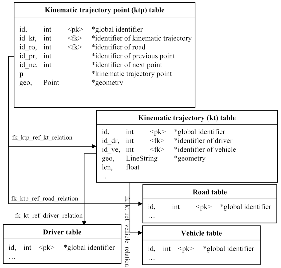
PostGIS [27] is chosen to develop our database system, in which three tables: kinematic trajectory point (ktp) table, kinematic trajectory (kt) table and road table of HD maps are mainly used, as Figure 2 shows. The ktp table stores key kinematic information of these points. The topological information of kinematic points is also maintained in this table. For example, the ID of the road a kinematic point is located in can be easily known from the ktp table. The id_ro attribute is used to screen out unrelated points in a spatial search when a vehicle is driving on the road. This would speed up our queries. In addition, generalized search tree indexes are built on the ktp table to further accelerate the queries. We use id_kt to link the ktp table to the kt table, in which the statistic of the trajectories and semantic information of kinematic points are stored. The driver and vehicle table maintains the personal/private information of registered drivers and vehicles.
In this paper, we assume that a global route is planned in advance. Therefore all the roads that a vehicle will pass through can be known. In a query, only data linked to the roads are scanned.

4.2.2. Adaptive Spatial Retrieve Algorithm (ASRA)

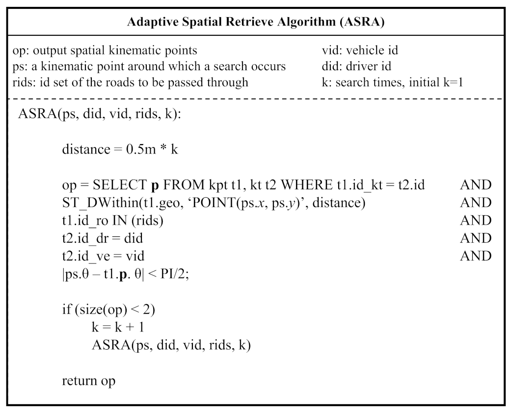
Kinematic trajectory points are not uniformly distributed in space; thus, it is unsuitable to use a fixed distance threshold in spatial searches. A recursive spatial retrieve algorithm is proposed. The algorithm adaptively sets the search distance to ensure that at least two associated kinematic trajectory points can be found. Its pseudocodes are shown in Figure 3.
Based on Tobler’s first law of geography, ASRA tries to find the closest associated kinematic points. Namely, around a specified position (ps.x, ps.y), the associated kinematic trajectory points must comply with the following rules:
  • Spatial rules: the points must be within a certain distance 0.5 m * k, where k < 5, and the heading difference must be less than π / 2 ; otherwise, the points are kicked out; if k ≥ 5 and the point number is less than 2, the search fails.
  • Topological rules: the points must be located on the road that the vehicle is driving on; otherwise, the points are kicked out.
  • Semantic rules: the points must be produced by the same vehicle that is driven by the same person; otherwise, the points are kicked out.
The topological rules screen out plenty of unconcerned points to speed up the search. The spatial rules select all surrounding points that have a close heading angle within a certain distance. The semantic rules ensure only private data are selected. On the one hand, this protects the privacy of drivers; on the other hand, it is the key of personalized predictions. The searched kinematic points op are used to calculate virtual measurements in the following prediction algorithm. The details can be found in the section “(Process 2) Spatial Search and Virtual Measurement Calculation”.

4.2.3. EKF Framework for Kinematic Trajectory Data Integration

As reported in our previous work [12], the accuracy performances of EKF and UKF are almost identical; however, EKF is faster. Motion predictions are computation-consumed; the efficiency of an algorithm shall be seriously treated. Thus, an EKF that cooperates with the CTRV model is used in vehicle motion prediction.
In the CTRV model, an estimated vehicle state at instant k is defined as x ^ k = x y θ v ω T . In our system, the current vehicle state estimate x ^ k c t r a , which is output by the UKF, is assigned to x ^ k c t r v as the initial state of our EKF predictor through:
x ^ k c t r v = I 0 0 0 0 0 1 5 × 6 × x ^ k c t r a
Hereafter, we denote x ^ k c t r v as x ^ k for brevity.

(Process 1) Predicting

Firstly, the initial state x ^ k and the corresponding covariance P k have evolved into the next instant’s state x ^ k + 1 and covariance P k + 1 through Equations (4)–(6).
x ^ k + 1 = F c t r v ( x ^ k ) + w k
F c t r v ( x ^ k ) = x k + v k ω k sin ( θ k + ω k T ) v k ω k sin ( θ k ) y k v k ω k cos ( θ k + ω k T ) + v k ω k cos ( θ k ) θ k + ω k T v k ω k
P k + 1 = J F P k J F T + Q k
w k is the process noise. J F and Q k denote the Jacobian matrix of function F c t r v and the covariance matrix of process noise, respectively. For more details on the Jacobian and covariance matrices, see [12].

(Process 2) Spatial Search and Virtual Measurement Calculation

Secondly, we try to find the associated kinematic points around the predicted position and use these points to calculate a virtual measurement.
The ASRA is triggered around x ^ k + 1 and the associated kinematic trajectory points op are retrieved by ASRA. Then op is used to construct the following matrix:
op = x 1 y 1 θ 1 v 1 ω 1 x n y n θ n v n ω n T
where n is the element number of op and we use ( op ) i to denote the i-th column of op. Each column corresponds to an associated kinematic point. The following three weighting functions are proposed to calculated weights for each kinematic trajectory point.
w i j = w i ( d j ) = 1 d j j n d j , i = 1 1 , i = 2 e k d j , i = 3
where d j is the Euclidean distance between x ^ k + 1 and ( op ) j , defined in Equation (9).
d j = E D ( x ^ k + 1 , ( op ) j ) = ( x x x op ) 2 + ( y x y op ) 2
The three weighting functions are illustrated in Figure 4; we can see that w 2 is an average weighting (AW) method; both w 1 and w 3 are inverse distance-weighting (IDW) methods, while w 1 is linear and yet w 3 is nonlinear. The weights are then normalized through Equation (10).
w i j = w i j j = 1 n w i j , where i { 1 , 2 , 3 }
Using the calculated weights w i j , the weighted mean of the queried associated kinematic trajectory points is regarded as a virtual measurement z k + 1 v i r t u a l , as expressed in Equation (11).
z k + 1 v i r t u a l = op × w i 1 w i 2 w i n T , where i { 1 , 2 , 3 } and j { 1 , 2 , , n }
Obviously, our measurement function is:
z k + 1 = x k + 1 + e k + 1
where e k + 1 is the measurement noise.

(Process 3) Updating

Finally, the virtual measurement derived from Process 2 is used to update the prediction made by Process 1 in this process. First of all, the near-optimal Kalman gain G k + 1 is calculated by:
G k + 1 = P k + 1 J H T ( J H P k + 1 J H T + R k + 1 ) 1
where J H = I and R k + 1 is the covariance matrix of e k + 1 . Then, the state prediction is corrected by the virtual measurement through:
x ^ k + 1 = x ^ k + 1 + G k + 1 ( z k + 1 v i r t u a l x ^ k + 1 )
and the a posteriori estimate covariance matrix is given by:
P k + 1 = ( I G k + 1 J H ) P k + 1
The above process, from Equation (4) to Equation (15), is iterated 50 times to predict vehicle motions 5 s into the future.

5. Experiments

5.1. Experimental Configurations

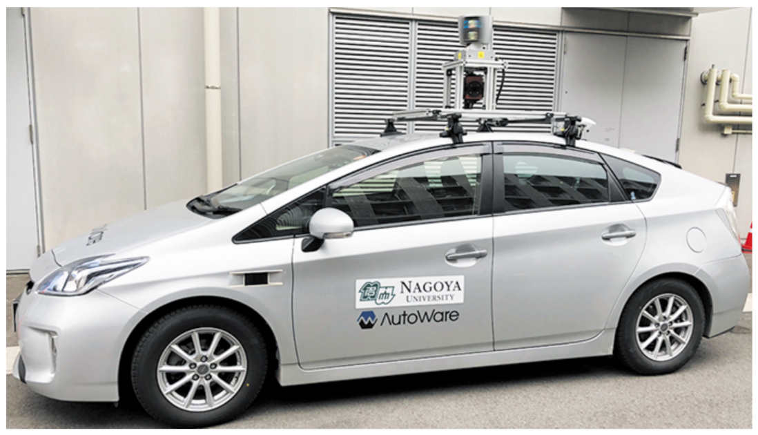
Real-world experiments were conducted on the campus of Nagoya University using the Toyata PRIUS PHV shown in Figure 5. The LiDAR (Velodyne HDL-64ES3) and the IMU (inertia measurement unit, Xsens MTi-300) mounted on the vehicle were used in our experiments. The sensors were connected to the Autoware platform [28,29,30] and our system subscribed to the ROS (Robot Operating System) [31] messages published by the sensor nodes to estimate vehicle state and predict vehicle motion.
It is noteworthy that our experiments were conducted in a public space where the roads were curved and sloped and pedestrians, bikes and other vehicles coexisted. This made our driving behaviors complex; for example, we had to stop our car when pedestrians crossed the road and depart the planed lane when a vehicle parked on the road side. In our experiments, three drives’ kinematic data, 12,112 points in total, were stored in the database and the other one was replayed to duplicate the real driving, as we had done in [14].
Our system was implemented based on C++ and ROS. Details of the configurations of experimental vehicle, sensors and KFs can be found in [12].

5.2. Accuracy Performance Evaluations

Two factors that might impact our algorithm’s accuracy performance—the used weighting function and data set size—are investigated in this section.

5.2.1. Used Metrics

The accuracy performance of our method is evaluated quantitatively, using the average Euclidean error (AEE) and max error metrics. AEE is used to analyze the overall prediction performance of our algorithm and is defined as:
A E E ( t i ) = 1 N j = 1 N ( x t i j x t i r ) 2 + ( y t i j y t i r ) 2
where ( x t i j , y t i j ) is the predicted position at time t i along the j t h predicted trajectory. ( x t i r , y t i r ) is the corresponding real position. N is the total number of predicted trajectories. The velocity prediction errors are also calculated with the AEE method; however, it is one-dimensional:
v e l o c i t y e r r o r ( t i ) = 1 N j = 1 N | v t i j v t i r |
Similarly, v t i j and v t i r are predicted and real velocity at time t i along the j t h predicted trajectory, respectively.
Max error is the max prediction error along a predicted trajectory. The max error reflects the worst performance in a single trajectory prediction. Therefore, it can reveal some factors covered by the mean values that are derived from the overall predictions. More than 10,000 trajectories were predicted in each of following experiments and their prediction errors were discussed in detail.

5.2.2. Using Different Weighting Functions

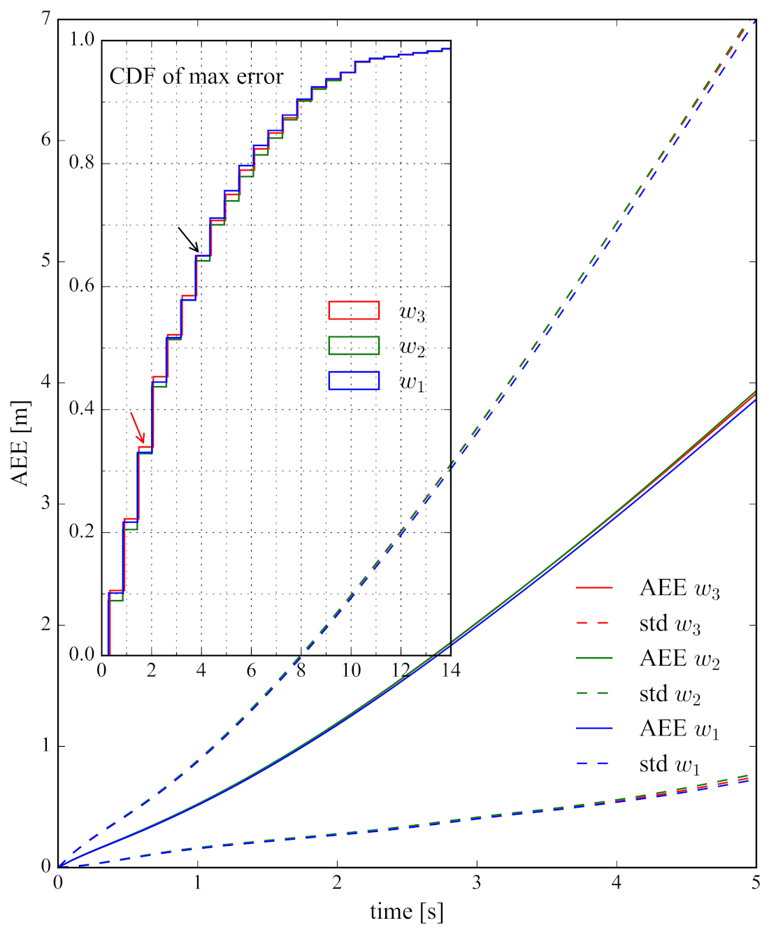
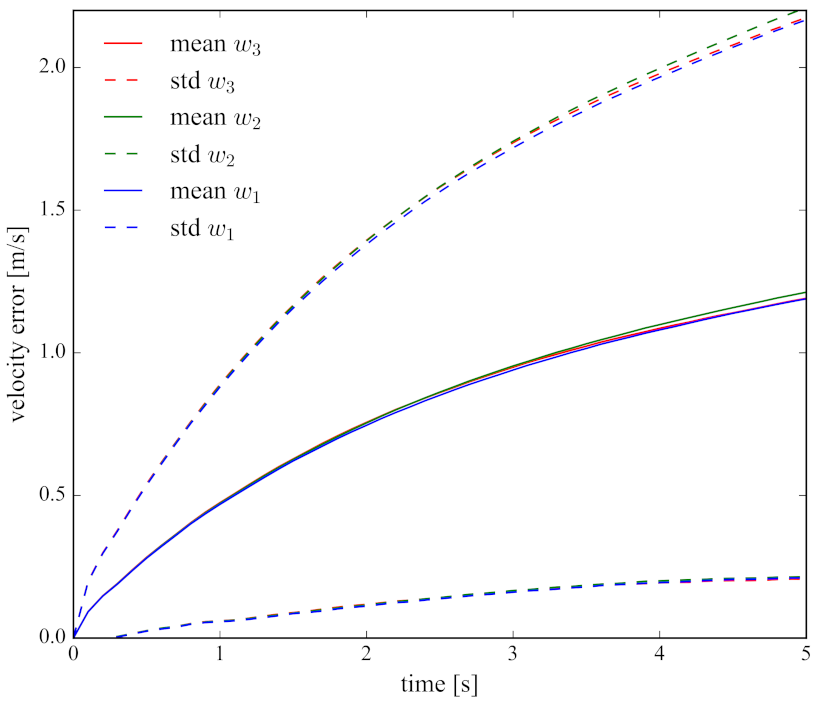
In order to investigate the impact of different weighting functions, the prediction accuracy performance of three predictors that used different weight functions, w 1 , w 2 and w 3 , were compared. In this experiment, all the collected kinematic trajectory data in our database were used. The experimental results are shown in Figure 6 and Figure 7.
An obvious trend can be found—the three weighting functions have not made a distinct difference in accuracy aspect, for both position and velocity predictions. However, the IDW methods ( w 1 and w 3 ) are slightly better than the AW method ( w 2 ) in either position or velocity predictions. This is because our search radius is small (initial radius is 0.5 m and max search radius is not more than 2 m); the spatial differences among the searched kinematic trajectory points are therefore slight. Thus, different weighting functions cannot lead to obvious differences from a statistical standpoint. Compared with the state-of-the-art method in [13], whose position and velocity prediction errors are more than 4 m and 1.5 m/s at 4 s respectively, the performance of our method is acceptable.
For a further and meticulous investigation of prediction errors, their max prediction errors are analyzed. The max errors’ cumulative distribution functions (CDFs) when the three different weighting functions are used are drawn in the upper-left corner in Figure 6. We divide the max prediction errors into four groups: outstanding (max error ≤ 2 m), good (2 m < max error ≤ 4 m), not bad (4 m < max error ≤ 7 m) and bad (max error > 7 m). The four max error groups’ spatial distributions can be found in Figure 8.
From the CDFs in Figure 6, we can find that good predictions, including outstanding predictions, make up more than 60% using either weighting function, as the black arrow indicates. This means the good prediction rate of our method is over 60% in our complex experimental space. It is also noticeable, where the red arrow points, that w 3 (the red) yields a higher rate (34%, approximately) of outstanding predictions. Therefore, to obtain more outstanding predictions, w 3 is recommended.

5.2.3. Using Different Data Sets

As mentioned before, the learning-based methods consume plenty of historical data; the model’s performance is determined by the size of HDT. The following experiments are designed to answer two questions: (1) How does our method perform when the historical data that can be used are limited? For example, in the condition where just one trajectory is available. (2) How does our method perform when the size of historical data increases? The first question indicates the worst performance of our method in bad conditions. The second question assesses the performance potential of our method in good conditions.
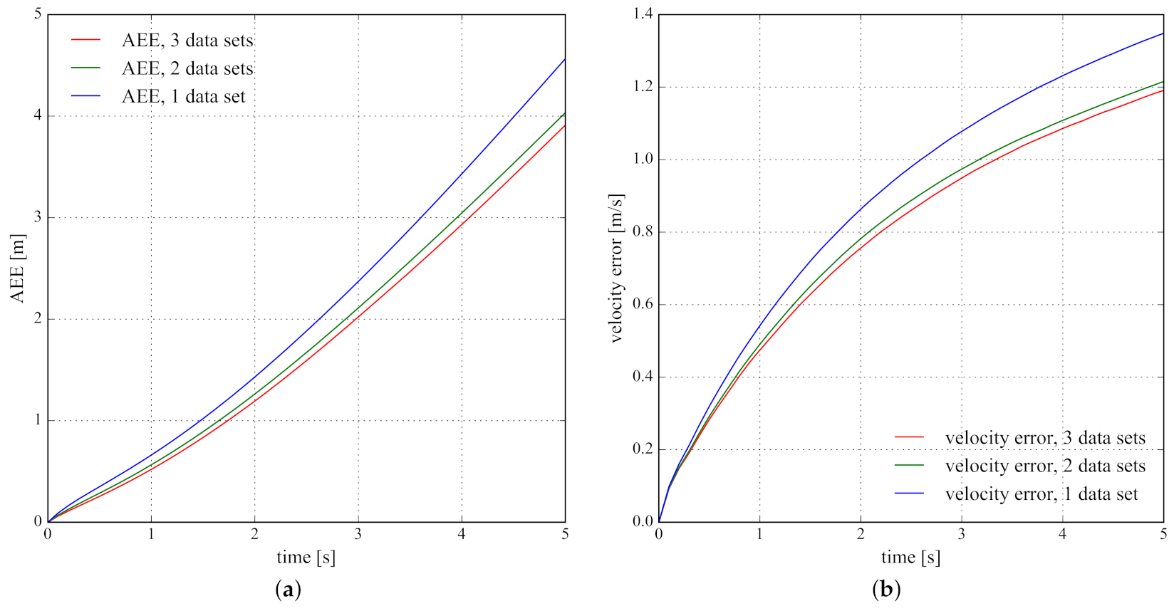
We had collected three kinematic trajectory data sets { K T 1 , K T 2 , K T 3 } in our database. Each trajectory data set corresponded to a drive on the route in Figure 8 in our campus. Some information about the trajectories are listed in Table 2. Using w 3 , our method was tested on different data sets, including one data set { { K T 1 } , { K T 2 } , { K T 3 } } that involves three experiments, two data sets { { K T 1 , K T 2 } , { K T 1 , K T 3 } { K T 2 , K T 3 } } that involve three experiments and three data sets { { K T 1 , K T 2 , K T 3 } } that involve one experiment. Their average prediction errors are summarized in Figure 9.
For the second question, Figure 9 clearly shows that with the size of the used data sets increased, the prediction accuracy of both position and velocity is improved. This figure reveals the promising application of our method in the future when collected trajectory data substantially increase. It can be inferred that the accuracy performance can be further improved if more data sets were utilized. After all, achieving that significant accuracy performance, only three data sets were used at most.
For the first question, in Figure 9, an important point that should be noticed is that in the worst cases where just one data set was used, the prediction performance of our method (the blue curves) was acceptable, compared with the reported accuracy in [13]. This also proves that our method is not data-consumed. The more data sets utilized, the better our approach performs.

5.3. Efficiency Performance Evaluations

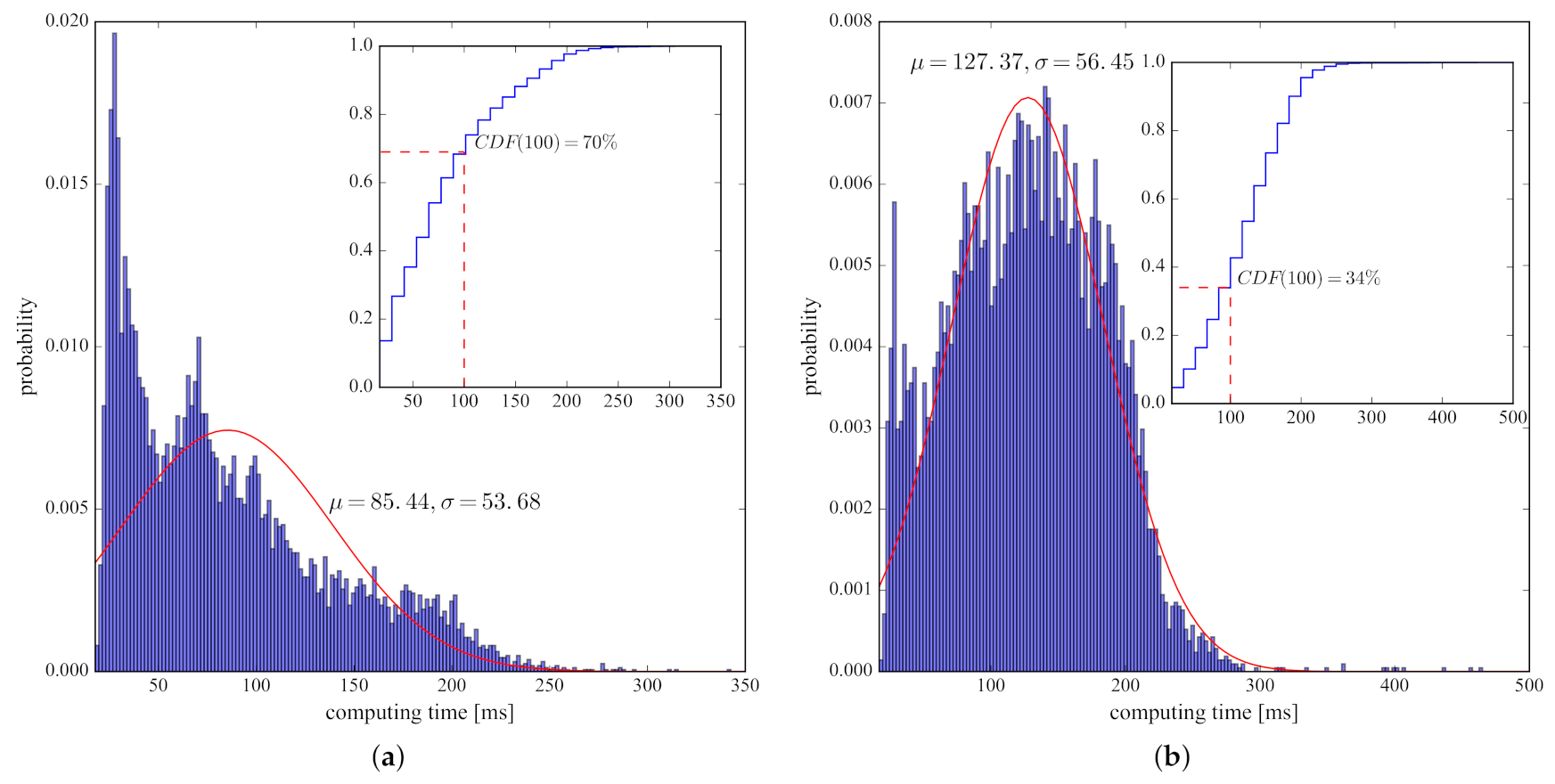
In most of the presented studies, efficiencies of algorithms were rarely discussed due to most learning-based LVMP methods not being lightweight. In our previous work, it was forecasted that with the amount of computations increased, EKF that has almost the same accuracy as UKF may remarkably outperform UKF in efficiency [12]. This experiment was designed to investigate the efficiency of our method; on the other hand, we want to validate our previous forecast. In the below experiments, both EKF and UKF predictors were implemented; they cooperated with the same CTRV model and w 3 weighting function and were tested on the same three data sets. Each experiment was repeated three times and the computing-time statistics are presented in Figure 10.
As the figures show, the EKF predictor (mean computing time: 85 ms) is obviously faster than the UKF predictor (mean computing time: 127 ms). As our vehicle state estimator works at 10 Hz, from the figures, we can roughly figure out that 70% EKF predictions are accomplished in time (CDF (100 ms) = 70%), while only 34% UKF predictions are accomplished in time (CDF (100 ms) = 34%).
In practice, the UKF predictor would lose many predictions in estimation-prediction cycles, and for some vital ADAS applications, such as collision detection, prediction data absence is a critical defect. UKF is thus not recommended in our system.

6. Future Work

This paper is a preliminary for implementing the proposed system. There are several tasks remaining for future study.
Firstly, as the above experiments indicates, the prediction accuracy is improved with the size of used data sets increased; therefore, the extreme accuracy of our method shall be investigated by increasing our data sets substantially. In addition, data sets’ interoperability between different vehicles and drivers shall also be examined.
Secondly, the spatial distributions of the four max error groups are shown in Figure 8. Unfortunately, we have not found a clear spatial distribution pattern so far. In order to improve the performance of our method, the spatial distribution patterns and the issues that affect the performance of our method shall be studied.
Finally, with the size of collected data dramatically increased in the future, a new computing framework is demanded, as we did in [14].

7. Conclusions

A novel lightweight LVMP method was proposed in this paper. Kinematic trajectory data were the result of interactions between humans, vehicles and environments. The kinematic trajectory data were directly used in our LVMP method and they were managed by a spatial database. A new KF framework that cooperated with the spatial database system was proposed to achieve LVMP in real time. Our method was validated in the real world. The proposed IDW methods showed slight advantage in accuracy, compared with the AW method. The size of the used data sets impacts the accuracy performance of our method. The experiments showed that as the used data sets increased, the prediction accuracy was improved, and our method was not data-consumed. Concerning the efficiency aspect, our method could meet real-time prediction requirements; the EKF predictor runs much faster than the UKF predictor, which hardly predicted in real time and thus was not recommended.

Author Contributions

Conceptualization, Lu Tao; methodology, Lu Tao.; software, Lu Tao; validation, Lu Tao; formal analysis, Lu Tao.; investigation, Lu Tao; resources, Yousuke Watanabe, Hiroaki Takada; data curation, Lu Tao; writing—original draft preparation, Lu Tao; writing—review and editing, Lu Tao; visualization, Lu Tao; supervision, Yousuke Watanabe, Hiroaki Takada; project administration, Hiroaki Takada; funding acquisition, Yousuke Watanabe, Hiroaki Takada. All authors have read and agreed to the published version of the manuscript.

Funding

This research was funded by JSPS KAKENHI grant number JP20H00589.

Institutional Review Board Statement

Not applicable.

Informed Consent Statement

Not applicable.

Data Availability Statement

Not applicable.

Conflicts of Interest

The authors declare no conflict of interest.

References

  1. Pihrt, J.; Šimánek, P. Spatiotemporal Prediction of Vehicle Movement Using Artificial Neural Networks. In Proceedings of the 2022 IEEE Intelligent Vehicles Symposium (IV), Aachen, Germany, 4–9 June 2022; pp. 734–739. [Google Scholar] [CrossRef]
  2. Lefèvre, S.; Vasquez, D.; Laugier, C. A survey on motion prediction and risk assessment for intelligent vehicles. Robomech J. 2014, 1, 1. [Google Scholar]
  3. Tan, H.S.; Huang, J. DGPS-Based Vehicle-to-Vehicle Cooperative Collision Warning: Engineering Feasibility Viewpoints. IEEE Trans. Intell. Transp. Syst. 2006, 7, 415–428. [Google Scholar]
  4. Lytrivis, P.; Thomaidis, G.; Tsogas, M.; Amditis, A. An Advanced Cooperative Path Prediction Algorithm for Safety Applications in Vehicular Networks. IEEE Trans. Intell. Transp. Syst. 2011, 12, 669–679. [Google Scholar]
  5. Hermes, C.; Wohler, C.; Schenk, K.; Kummert, F. Long-term Vehicle Motion Prediction. In Proceedings of the Intelligent Vehicles Symposium, Xi’an, China, 3–5 June 2009. [Google Scholar]
  6. Jeong, D.; Baek, M.; Lee, S.S. Long-term prediction of vehicle trajectory based on a deep neural network. In Proceedings of the International Conference on Information & Communication Technology Convergence, Jeju, Korea, 18–20 October 2017. [Google Scholar]
  7. Altché, F.; de La Fortelle, A. An LSTM network for highway trajectory prediction. In Proceedings of the 2017 IEEE 20th International Conference on Intelligent Transportation Systems (ITSC), Yokohama, Japan, 16–19 October 2017; pp. 353–359. [Google Scholar] [CrossRef]
  8. Jiang, R.; Xu, H.; Gong, G.; Kuang, Y.; Liu, Z. Spatial-Temporal Attentive LSTM for Vehicle-Trajectory Prediction. ISPRS Int. J. Geo-Inf. 2022, 11, 354. [Google Scholar] [CrossRef]
  9. Lin, L.; Li, W.; Bi, H.; Qin, L. Vehicle Trajectory Prediction Using LSTMs with Spatial-Temporal Attention Mechanisms. IEEE Intell. Transp. Syst. Mag. 2022, 14, 197–208. [Google Scholar] [CrossRef]
  10. Petrich, D.; Dang, T.; Kasper, D.; Breuel, G.; Stiller, C. Map-based long term motion prediction for vehicles in traffic environments. In Proceedings of the 16th International IEEE Conference on Intelligent Transportation Systems (ITSC 2013), The Hague, The Netherlands, 6–9 October 2013. [Google Scholar]
  11. Yalamanchi, S.; Huang, T.K.; Haynes, G.C.; Djuric, N. Long-term prediction of vehicle behavior using short-term uncertainty-aware trajectories and high-definition maps. In Proceedings of the 2020 IEEE 23rd International Conference on Intelligent Transportation Systems (ITSC), Rhodes, Greece, 20–23 September 2020; pp. 1–6. [Google Scholar]
  12. Lu, T.; Watanabe, Y.; Yamada, S.; Takada, H. Comparative evaluation of Kalman filters and motion models in vehicular state estimation and path prediction. J. Navig. 2021, 74, 1142–1160. [Google Scholar]
  13. Kawasaki, A.; Tasaki, T. Trajectory Prediction of Turning Vehicles based on Intersection Geometry and Observed Velocities. In Proceedings of the IEEE Intelligent Vehicles Symposium, Changshu, China, 26–30 June 2018; pp. 511–516. [Google Scholar]
  14. Tao, L.; Watanabe, Y.; Li, Y.; Yamada, S.; Takada, H. Collision Risk Assessment Service for Connected Vehicles: Leveraging Vehicular State and Motion Uncertainties. IEEE Internet Things J. 2021, 8, 11548–11560. [Google Scholar] [CrossRef]
  15. Hafner, M.R.; Cunningham, D.; Caminiti, L.; Vecchio, D.D. Cooperative Collision Avoidance at Intersections: Algorithms and Experiments. IEEE Trans. Intell. Transp. Syst. 2013, 14, 1162–1175. [Google Scholar] [CrossRef]
  16. Joerer, S.; Segata, M.; Bloessl, B.; Cigno, R.L.; Sommer, C.; Dressler, F. A Vehicular Networking Perspective on Estimating Vehicle Collision Probability at Intersections. IEEE Trans. Veh. Technol. 2014, 63, 1802–1812. [Google Scholar] [CrossRef]
  17. Shan, M.; Worrall, S.; Nebot, E. Long Term Vehicle Motion Prediction and Tracking in Large Environments. In Proceedings of the IEEE International Conference on Intelligent Transportation Systems (ITSC’11), Washington, DC, USA, 5–7 October 2011. [Google Scholar]
  18. Xu, Y.; Liu, X.; Cao, X.; Huang, C.; Liu, E.; Qian, S.; Liu, X.; Wu, Y.; Dong, F.; Qiu, C.W.; et al. Artificial intelligence: A powerful paradigm for scientific research. Innovation 2021, 2, 100179. [Google Scholar] [CrossRef]
  19. Quan, T.; Firl, J. Modelling of traffic situations at urban intersections with probabilistic non-parametric regression. In Proceedings of the Intelligent Vehicles Symposium, Gold Coast, QLD, Australia, 23–26 June 2013. [Google Scholar]
  20. Gindele, T.; Brechtel, S.; Dillmann, R. Learning Driver Behavior Models from Traffic Observations for Decision Making and Planning. Intell. Transp. Syst. Mag. IEEE 2015, 7, 69–79. [Google Scholar] [CrossRef]
  21. Zhang, K.; Feng, X.; Wu, L.; He, Z. Trajectory Prediction for Autonomous Driving Using Spatial-Temporal Graph Attention Transformer. IEEE Trans. Intell. Transp. Syst. 2022, 1–11. [Google Scholar] [CrossRef]
  22. Lu, Y.; Wang, W.; Hu, X.; Xu, P.; Zhou, S.; Cai, M. Vehicle Trajectory Prediction in Connected Environments via Heterogeneous Context-Aware Graph Convolutional Networks. IEEE Trans. Intell. Transp. Syst. 2022, 1–13. [Google Scholar] [CrossRef]
  23. Schmidt, J.; Jordan, J.; Gritschneder, F.; Dietmayer, K. CRAT-Pred: Vehicle Trajectory Prediction with Crystal Graph Convolutional Neural Networks and Multi-Head Self-Attention. In Proceedings of the 2022 International Conference on Robotics and Automation (ICRA), Philadelphia, PA, USA, 23–27 May 2022; pp. 7799–7805. [Google Scholar] [CrossRef]
  24. Baumann, U.; Guiser, C.; Herman, M.; Zollner, J.M. Predicting Ego-Vehicle Paths from Environmental Observations with a Deep Neural Network. In Proceedings of the IEEE International Conference on Robotics and Automation (ICRA), Brisbane, QLD, Australia, 21–25 May 2018. [Google Scholar]
  25. Tobler, W.R. A Computer Movie Simulating Urban Growth in the Detroit Region. Econ. Geogr. 1970, 46, 234–240. [Google Scholar] [CrossRef]
  26. Wan, E.A.; Merwe, R. The unscented Kalman filter for nonlinear estimation. In Proceedings of the Adaptive Systems for Signal Processing, Communications, and Control Symposium, Lake Louise, AB, Canada, 4 October 2000. [Google Scholar]
  27. PostGIS. Available online: http://www.postgis.org (accessed on 23 June 2022).
  28. Kato, S.; Takeuchi, E.; Ishiguro, Y.; Ninomiya, Y.; Takeda, K.; Hamada, T. An Open Approach to Autonomous Vehicles. IEEE Micro 2015, 48, 60–68. [Google Scholar] [CrossRef]
  29. Kato, S.; Tokunaga, S.; Maruyama, Y.; Maeda, S.; Hirabayashi, M.; Kitsukawa, Y.; Monrroy, A.; Ando, T.; Fujii, Y.; Azumi, T. Autoware on Board: Enabling Autonomous Vehicles with Embedded Systems. In Proceedings of the 2018 ACM/IEEE 9th International Conference on Cyber-Physical Systems (ICCPS), Porto, Portugal, 11–13 April 2018. [Google Scholar]
  30. Autoware. Available online: https://github.com/autowarefoundation/autoware (accessed on 7 August 2022).
  31. Robot Operating System. Available online: http://www.ros.org (accessed on 23 June 2022).
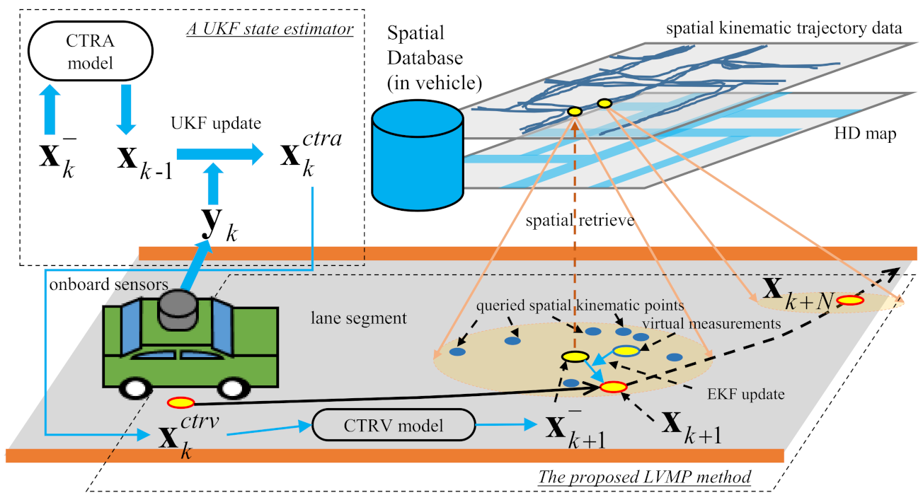
Figure 1. System overview. The idea of this paper is inspired by the first law of geography that everything is related to everything else, but near things are more related to each other.
Ijgi 11 00463 g001
Figure 2. The physical data model of spatial kinematic trajectory database, where * denotes explanations of the columns.
Ijgi 11 00463 g002
Figure 3. The proposed adaptive spatial retrieve algorithm.
Ijgi 11 00463 g003
Figure 4. The proposed weighting functions. w 1 is a linear IDW method; w 2 is an AW method; w 3 is a nonlinear IDW method.
Ijgi 11 00463 g004
Figure 5. The experimental vehicle. For more information about the vehicle, please refer to [28,29,30].
Ijgi 11 00463 g005
Figure 6. Statistics of position prediction errors. The solid and dotted lines are the AEEs and standard deviations (std) of position prediction errors, respectively. The red corresponds to the nonlinear IDW method w 3 ; the green corresponds to the AW method w 2 ; the blue corresponds to the linear IDW method w 1 . The IDW methods (red and blue) are slightly better than the AW method (green). The CDFs of max prediction errors when w 3 , w 2 , w 1 are used are plotted in the upper-left box. The red arrow indicates that w 3 yields more outstanding predictions. The black arrow indicates a good prediction rate of either weighting function in our algorithm of more than 60%.
Ijgi 11 00463 g006
Figure 7. Statistics of velocity prediction errors. The solid and dotted lines are the means and standard deviations (std) of velocity prediction errors, respectively. The red corresponds to the nonlinear IDW method w 3 ; the green corresponds to the AW method w 2 ; the blue corresponds to the linear IDW method w 1 . The IDW methods (red and blue) are slightly better than the AW method (green).
Ijgi 11 00463 g007
Figure 8. Spatial distribution of max prediction errors along the driving route.
Ijgi 11 00463 g008
Figure 9. Prediction errors using different data sets. An obvious trend can be found—with the size of used data sets increased, the prediction accuracy of both position and velocity is improved. (a) The position prediction error. The red, green and blue curve, respectively, correspond to the position-prediction errors using 3, 2 and 1 data sets. (b) The velocity prediction errors. The red, green and blue curve, respectively, correspond to the velocity-prediction errors using 3, 2 and 1 data sets.
Ijgi 11 00463 g009
Figure 10. Computing-time comparisons. The histograms and corresponding fitted normal distribution curves of computing time using EKF and UKF are given. μ is mean value and σ is standard deviation. In the upper-right boxes, the CDFs of computing time are given. The value of CDF(100) is the rate that the prediction is completed in real time. (a) The EKF predictor. (b) The UKF predictor.
Ijgi 11 00463 g010
Table 1. A comparison between our method and some typical methods selected from the five genres. The methods with learning/training processes are regarded as DCC.
StudyGenreInputOutputMethodologyScenarioDCCPersonalized
[4]physical model basedvehicle statepositionkinematic models, Dempster–Shafer reasoning systemcampusNoNo
[5]trajectory matching basedodometry data, HDT 1position, velocity, yaw and yaw angleparticle filter, trained trajectory classifierintersectionYesNo
[8]machine learning basedthe first 3 s historical trajectories, HDTpositionLSTMhighwayYesNo
[13]map-aidedHD maps, vehicle stateposition, velocityEKF, cubic polynomial fittingintersectionNoNo
[11]hybridHDT, HD mapspositionUncertainty-aware StitchingintersectionYesNo
oursspatial historical data basedvehicle state, spatial kinematic dataposition, velocityEKF, spatial searchcampusNoYes
1 HDT: Historical Data for Training.
Table 2. The kinematic statistics of the three drives.
TrajectoryMean v ( m / s )Std v ( m / s )Mean a ( m / s 2 )Std a ( m / s 2 )DriverVehiclePoint Number
K T 1 5.821392.654610.046190.62621YamataPHV0013895
K T 2 5.254372.238740.046690.51137YamataPHV0014142
K T 3 5.497082.015450.058260.47457YamataPHV0014075
Publisher’s Note: MDPI stays neutral with regard to jurisdictional claims in published maps and institutional affiliations.