Generalization of Linear and Area Features Incorporating a Shape Measure

Abstract

This article elaborates on the quality issue in cartographic generalization of linear and area features focusing on the assessment of shape preservation. Assessing shape similarity in generalization is still a topic where further research is required. In the study presented here, shape description and matching techniques are investigated and analyzed, a procedure for choosing generalization parameters suitable for line and area features depiction is described and a quality model is developed for the assessment and verification of the generalization results. Based on the procedure developed, cartographers will be confident that the generalization of linear and area features is appropriate for a specific scale of portrayal fulfilling on the same time a basic requirement in generalization, that of shape preservation. The results of the procedure developed are based on the processing and successful generalization of a large number of different line and area features that is supported by a software environment developed in Python programming language.

1. Introduction

This article elaborates on quality in cartographic generalization of linear and polygonal features and focuses on the issue of shape preservation, aiming to contribute to the research conducted in the framework of automation in map generalization. The presented study constitutes a part of wider research concerning quality assessment and evaluation of the generalized features in the two distinct phases of the map generalization process (semantic and cartographic generalization), as presented in [1]. Two main realizations are described in this article: (a) the identification of a shape measure for the assessment and evaluation of the shape preservation degree regarding linear and polygonal features generalized with simplification algorithms, and (b) a methodology for choosing the suitable line shape for portrayal at a specific map scale. In addition, the design of a functional quality model adequate for utilization in the cartographic generalization process is presented, which also serves as a tool for the verification of the suitability of the proposed measure. The quality model incorporates the proposed shape measure and selection methodology and includes the specifications pertinent to the scale of the map, with the measures adopted along with the corresponding thresholds and the quality controls for the evaluation of the cartographic generalization results. The outcome of the quality model is a proof of concept for the methodology developed.

1.1. Background in Evaluation of Map Generalization

Over the last decade, several national mapping agencies (Ordnance Survey of Great Britain (OSGB), UK, Institut Geographique National (IGN), France, The Netherlands Kadaster, Netherlands, Institut Cartografic de Catalunya (ICC), Spain, AdV, Germany, Swisstopo, Switzerland, KMS, Denmark, USGS, USA) have developed automated or semi-automated processes in the map production line [2,3,4,5]. Among them, the most thoroughly and persistently investigated process regards automation in map generalization.

A fundamental element in the evolution of map generalization process modeling has been the development of a quality evaluation mechanism which differentiates the earlier modeling methods (condition-action modeling, batch-mode modeling, human interaction modeling) from constraint-based modeling [6], which is currently incorporated in agent-based generalization systems (AGENT, CartACom, GAEL, RevK, CollaGEN). Their industrialized versions are utilized by certain European Mapping Agencies, with satisfactory results [5]. Constraint-based modeling, initially introduced by [7], is based on the idea of identifying a state in which a variety of constraints are satisfied [8]. This approach was elaborated in the framework of two major projects dedicated to automation in map generalization: (a) the AGENT project (1997–2000, IGN, France) and (b) the EuroSDR project (2006–2010). Along with these projects, two mutual complementary theories regarding evaluation process prevailed: the analysis of the evaluation process in three stages (evaluation for tuning, evaluation for controlling, evaluation for evaluation) [9] and the configuration of the three main components of automated evaluation ((a) definition and formalization of map requirements, (b) measures for automated evaluation regarding features’ geometric properties and relationships for detecting constraints violation and describing the violation’s severity, (c) data matching techniques between original and generalized data) [10].

Current studies [11] emphasize that high-impacting research on generalization with knowledge acquisition, constraint-based, agent-based, or optimization-based modeling is missing, and that the research on generalization models seems to be reaching its limits as parameterization becomes more complex. An approach concerning the incorporation of deep learning techniques in generalization modeling is emerging [11,12,13], but this research is in its infancy. Therefore, the research goals presented in this work focus on the improvement of the existing generalization models and, more specifically, on the constraint-based model.

1.2. Research Goals and Objectives

Although extensive research is being conducted on the evaluation of map generalization, in the acquisition of knowledge to form preservation constrains (e.g., shape), the definition of the violation of preservation and legibility constraints is deemed tolerable. It is therefore necessary to provide a formal description of tolerated violations [10], or to examine new simplified techniques for the resolution of geometric conflicts. It is estimated that in some cases, simpler techniques perform better than those incorporated in Multi-Agent Systems with complex parameterization and the need for high computing performance [5]. Considering the above, the work presented here aims to overcome (a) the limitations in identifying shape constraints through the configuration of a shape measure, and (b) the shape preservation and legibility constraint threshold ambiguity and agent-based model complexity, by proposing a simple methodology for the choice of the suitably generalized features. Shape, legibility, and horizontal accuracy measures along with a new procedure for the selection of the properly generalized features for cartographic portrayal are combined in the framework of a quality model, which utilizes existing knowledge in constraint-based modeling and automated evaluation, as indicated in the previous section.

In Section 2, a shape description measure for the evaluation of the degree of shape preservation in generalization is introduced along with an overview of the examined shape similarity measures and shape representation techniques. Results of the tested shape-matching techniques are correlated and conclusions are presented. In Section 3, a method for the selection of the suitable generalized linear and areal features for portrayal is developed, and in Section 4, the components of a quality model for the assessment of the generalized features quality are presented. In Section 5, the results of Section 2, Section 3 and Section 4 are summarized, and in the discussion in Section 6, emphasis is given to the contribution of the methodology developed to automation in cartographic generalization. Section 7 presents concluding remarks and suggests topics for future work.

2. Assessing Shape Preservation in Cartographic Generalization

The evaluation of a feature’s shape preservation degree in cartographic generalization requires a measure for assessing the difference between a feature’s initial shape and its shape after the application of this particular transformation. Shape matching deals with shape transformation and measurement of its similarity with the initial one, using a specific measure [14]. In the technical specifications of the basic quality measures of the AGENT system (IGN) [15], a feature’s shape is defined as its geometric form. Likewise, [14] uses the term shape for a geometrical pattern consisting of a set of points, curves, surfaces, etc. Considering these definitions and the fact that simplification algorithms and displacement as a result of generalization operate on a feature’s geometric properties, the assessment of the feature’s shape preservation in relation to its initial shape evolves through the use of a shape-matching technique. Additional measures regarding the evaluation of its legibility, horizontal accuracy, and topological accuracy contribute to the integrity of the process. Therefore, the identification of a measure assessing the degree of the feature’s shape preservation is based on the following three elements: (a) the quantified parametric description of the feature’s shape using a description or representation technique; (b) the application of a shape-matching technique that uses a similarity measure to evaluate possible dissimilarity through the computation of a distance, which implies that a short distance means minor dissimilarity [14]; and (c) legibility measures (minimum distances between vertices, identification of ‘bottleneck’ phenomenon and sharp corners), horizontal accuracy, and topological consistency measures (identification of self-intersections and self-overlaps).

2.1. Shape Description and Representation Techniques

A description of a shape of a linear or area feature can be achieved through the mathematical representation of its geometric form or pattern, considering the above-mentioned definition of shape. In the technical specifications of the basic quality measures of the AGENT system (IGN) [15], linear and polygonal shape measures based on past research are summarized in groups regarding size, sinuosity/complexity, elongation/eccentricity, compactness, and other special factors (

Table 1. Copy of the AGENT measures [15] showing linear and polygonal shape measures used in past research summarized in groups.

Size	Sinuosity/Complex	Elongation/Eccentricity	Compactness	Important Aspects
Length	Measures on angularity	Brown eccentricity	Convex deficiencies	Minimum width parts of a building
Area	Curvilinearity measures	Elongation	Bending energy	Neck searching
Perimeter	Maximum bend height	Regnauld elongation	Miller’s measure	Bend shape
Bend height	Slope density function	Spreadness	Boyce–Clark radial shape index	Bend description
Maximum bend height	Richardson plot	Circularity	Compactness measures	Distance–direction matrix
Minimum width of polygon	Entropy Sinuosity	Ellipticity	Squareness	Number of points
Minimum bounding rectangle	Fourier descriptors	Moments	Wall squareness	Shortest edge
Coalescence of line	Density of coordinates
Coalescence conflict detection	Ratio of maximum chord
Epsilon band	Fractal dimension
Turning distance	Number of bends
Radial distance

). Another parameterization approach for line shape description with three variables (the average magnitude angularity at different vertex ranges, the error variance, and the ratio of line length to anchor line length) was proposed by [16]. This work compares the shape measures proposed by [17,18].

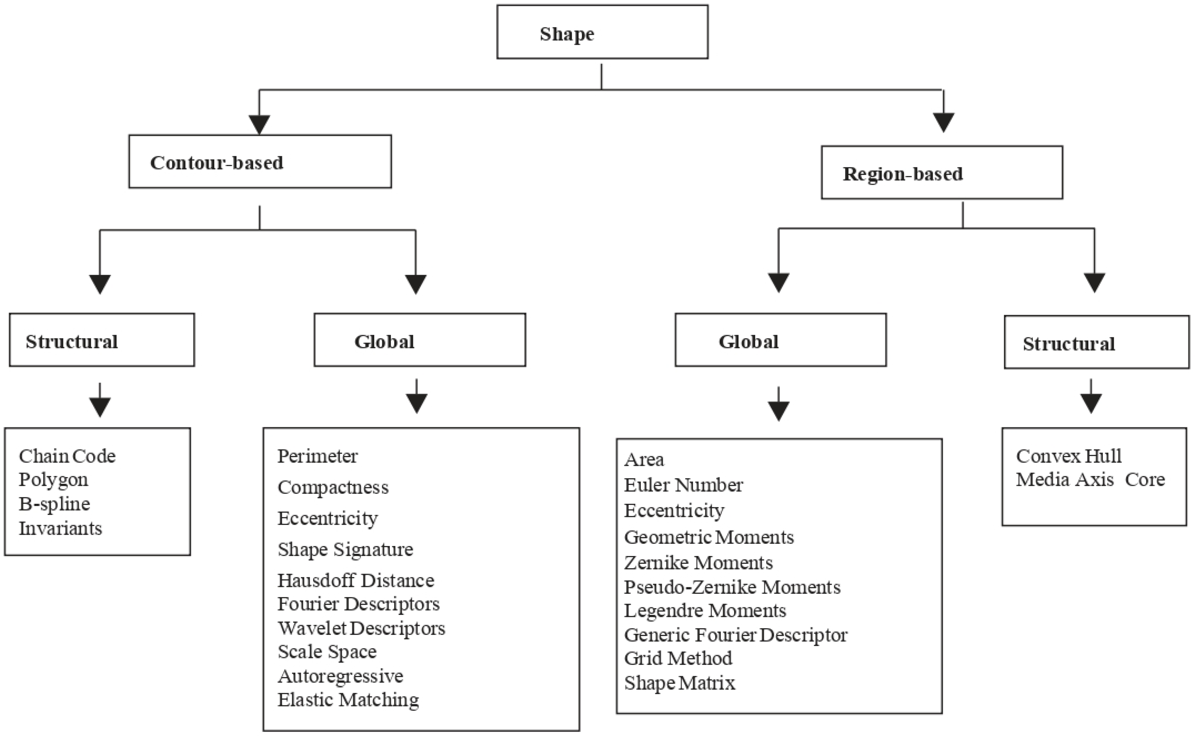
The following general categories and subcategories of shape description and representation techniques are suggested by [19]: (a) contour-based methods (global/structural) and (b) region-based methods (global/structural) (Figure 1).

In this work, aiming to identify an appropriate measure for the assessment of a line’s shape preservation degree, contour-based global methods (methods based on a feature’s “silhouette” that treat shape as a whole) are examined. Structural methods are not examined because of their computational complexity, complex matching, and failure to capture the global feature’s shape due to requiring the breakdown of the feature into segments (primitives) [19]. In the following section, the examined shape description and representation approaches are presented as part of the shape-matching methodologies.

2.2. Similarity Measures

The shape matching problem is considered to be twofold [14]: (a) the dissimilarity computation of two geometrical patterns (computation problem) and (b) the dissimilarity comparison using a threshold (decision/optimization problem). Furthermore, [14] refers to the following similarity measures that treat shape as a whole: discrete metric, Minkowski Lp, bottleneck distance, Hausdorff distance, Fréchet distance, turning function distance, nonlinear elastic matching distance, reflection distance, area of symmetric difference/template metric, and transport earth mover’s distance. This work focuses on the first component of the problem and examines the following shape-matching methods with the corresponding shape description or representation techniques and similarity measures: (a) Hausdorff distance, (b) modified Hausdorff distance, (c) discrete Fréchet distance, (d) turning function distance, and (e) distance between Fourier descriptors. Two basic criteria for the assessment of the examined similarity measures suitability are set: (a) any change in a feature’s spatial information (e.g., number of vertices) must correspond to a change in the value of the similarity measure, and (b) spatial information reduction is considered as shape distortion; therefore, an increase in the value of the similarity measure is expected, implying dissimilarity [14]. At this point, it must be clarified that the results regarding the similarity measures’ suitability are discussed in the framework of the assessment of the generalized feature shape, which, in most cases, is to a certain extent differentiated provided that the aims of generalization algorithms include the preservation of the feature shape. Therefore, the examined similarity measures which fail to follow the previously set criteria are not considered suitable for implementation in the generalization process. This does not imply, in general, a lack of their suitability to capture the features’ shape in cases where the shapes of two completely different features are examined.

In the following sections, the examined similarity measures are briefly described along with the representation techniques to be applied. Douglas–Peucker simplification algorithm for lines and polygons was chosen for testing the similarity measures as it can induce slight to great morphological distortions according to the set tolerance. Generalization was applied on a sample of 50 lines of 50 km each and 50 polygons (2.4–262 km²). These features are included in the EuroRegional Map database at scale 1:250,000. Douglas–Peucker simplification algorithm tolerance was set in the interval [20 m, 1000 m] per 20 m of length for the production of generalized features at scales 1:500,000 and 1:1,000,000. In addition, the bend simplification algorithm was applied for testing only the prevailed shape measures. Based on the function of the Douglas–Peucker simplification algorithm, one more criterion for the assessment of the examined similarity measures suitability was set: a quantitative increase in the values of the similarity measures is to be expected as the algorithm tolerance increases following the feature’s spatial information reduction (vertices). ESRI’s Douglas–Peucker simplification algorithm and bend simplification algorithm were implemented. The examined shape representation methods (turning function and line and polygon representation for Fourier transform) and the similarity measures (Hausdorff distance, modified Hausdorff distance, discrete Fréchet distance, turning function distance, Fourier descriptors distance) were implemented in Python programming language. Fourier descriptors were calculated using Inverse Fast Fourier Transform function in the Scipy Python module. The Shapely Python module was also used for buffering, area calculations, and examination of topological relationships.

2.2.1. Hausdorff Distance

Hausdorff distance between two sets of points A and B is defined as the smallest value d such that every point of A has a point of B within distance d and every point of B has a point of A within distance d [20].

$$\begin{gathered} \mathrm{H}\left(\mathrm{A},\mathrm{B}\right)=\max \left\{{\max }_{\mathrm{a}\in \mathrm{A}}{\min }_{\mathrm{b}\in \mathrm{B}}\left|\mathrm{b}-\mathrm{a}\right|,{\max }_{\mathrm{b}\in \mathrm{B}}{\min }_{\mathrm{a}\in \mathrm{A}}\left|\mathrm{a}-\mathrm{b}\right|\right\}, \\ \left|\mathrm{b}-\mathrm{a}\right|\mathrm{and}\left|\mathrm{a}-\mathrm{b}\right|\mathrm{are}\mathrm{the}\mathrm{Euclidean}\mathrm{distances} \end{gathered}$$

This specific measure was rejected because it is not able to capture slight changes in feature shape since coarse grouping is created, as it is derived from

Table 2. Computation of Hausdorff distances per tolerance value (line #1027).

Hausdorff Distance (m)	Number of Vertices	Tolerance Value (m)
0.000	994	0
591.692	184	20
591.692	126	40
904.121	100	60
904.121	85	80
904.121	73	100
904.121	64	120
904.121	56	140

.

2.2.2. Modified Hausdorff Distance

Other researchers have examined various alternatives to the Hausdorff distance [21], concluding that the following mathematical expression of the Hausdorff distance (modified Hausdorff distance) is a more suitable shape similarity measure. The modified Hausdorff distance between lines A and B is defined as follows:

$$\mathrm{f}\left(\mathrm{d}\left(\mathrm{A},\mathrm{B}\right),\mathrm{d}\left(\mathrm{B},\mathrm{A}\right)\right)=\max \left(\mathrm{d}\left(\mathrm{A},\mathrm{B}\right),\mathrm{d}\left(\mathrm{B},\mathrm{A}\right)\right)$$

• $\mathrm{d}\left(\mathrm{A},\mathrm{B}\right)=\frac{1}{\mathrm{Na}}{{\displaystyle \sum }}_{\mathrm{a}\in \mathrm{A}}\mathrm{d}\left(\mathrm{a},\mathrm{B}\right)$, the distance between the set of points on line A and the set of points on line B
• $\mathrm{d}\left(\mathrm{B},\mathrm{A}\right)=\frac{1}{\mathrm{N}\mathsf{\beta }}{\displaystyle \sum }_{\mathrm{b}\in \mathsf{{\rm B}}}\mathrm{d}\left(\mathrm{b},\mathsf{A}\right)$, the distance between the set of points on line B and the set of points on line A
• Na, Νβ = the number of points in each set of points on lines A and B
• $\mathrm{d}\left(\mathrm{a},\mathrm{B}\right)=\min \left|\right|\mathrm{a}-\mathrm{b}\left|\right|,$
  the minimum Euclidean distance between point a on line A and the set of points on line B
• $\mathrm{d}\left(\mathrm{b},\mathrm{A}\right)=\min \left|\right|\mathrm{b}-\mathrm{a}\left|\right|,$
  the minimum Euclidean distance between point b on line B and the set of points on line A

This specific measure was accepted as a similarity measure because of its property of following shape line changes: (a) it changes when line spatial information (line vertices) change, and (b) it increases following line shape distortion when the tolerance value increases (

Table 3. Computation of modified Hausdorff distances per tolerance value (line #1027).

Modified Hausdorff Distance (m)	Number of Vertices	Tolerance Value (m)
0.000	994	0
79.327	184	20
107.962	126	40
143.954	100	60
169.066	85	80
198.730	73	100
219.037	64	120
250.813	56	140

).

2.2.3. Discrete Fréchet Distance

The Fréchet distance between two curves f:[α,α′}, g:[b,b′] is described by the following function [22]:

${\mathsf{\delta }}_{\mathrm{F}}\left(\mathrm{f},\mathrm{g}\right)={\inf }_{\begin{array}{c}\mathsf{\alpha }\left[0,1\right]\to \left[\mathsf{\alpha },{\mathsf{\alpha }}^{\prime }\right]\\ \mathsf{\beta }\left[0,1\right]\to \left[\mathrm{b},{\mathrm{b}}^{\prime }\right]\end{array}}{\max }_{\mathrm{t}\in \left[0,1\right]}\Vert \mathrm{f}\left(\mathrm{a}\left(\mathrm{t}\right)\right)-\mathrm{g}\left(\mathsf{\beta }\left(\mathrm{t}\right)\right)\Vert$, where a, β range over continuous and increasing functions with α(0) = α, α(1) = α′, β(0) = b, β(1) = b′.

An alternative of Fréchet distance, the discrete Fréchet distance, is described as coupling distance [23]. Its computation includes the examination of all coupling distances between the end points of line segments of the polygonal curves, with the restriction that the backward computation is prohibited. Mathematically, the discrete Fréchet distance is described as follows:

${\mathsf{\delta }}_{\mathrm{dF}}\left(\mathrm{P},\mathrm{Q}\right)=\min \left\{\mathrm{L}\right\},$ where P, Q are the polygonal curves and ||L|| is the length of the longest link in the coupling L.

Discrete Fréchet distance computation between two polygonal curves P (p₀,…p_m), Q(q₀,….q_n) is based on the creation of an array ca (nxm), with distances calculated between polygonal curves vertices as in the following algorithm:

• i,j = 0 → ca(c₀₀) = d(p₀,q₀), the Euclidean distance between vertices p₀,q₀.
• i = 0 and j ϵ [1,n] → ca(c_0,j) = max{d(p₀,q_j),ca(c_0,j−1)}
• i ϵ [1,m] and j = 0 → ca(c_i,0) = max{d(p_i,q₀),ca(c_i−1,0)}
• i ϵ [1,m], j ϵ [1,n] → ca(c_i,j) = max(d(p_i,q_j), min{ca(c_i−1,0), ca(c_0,j−1), ca(c_i−1,j−1)})

The discrete Fréchet distance is the value in the lower right corner of the array ca (cell number nm) [24].

The numerical results of the discrete Fréchet distance application indicate its increasing tendency in relation to an increase in tolerance value of the generalization algorithm. However, coarse grouping occurs when slight differences in feature shape appear (

Table 4. Computation of discrete Fréchet distances per tolerance value (line #1027).

Discrete Frechet Distance (m)	Number of Vertices	Tolerance Value (m)
0.000	994	0
591.692	184	20
591.692	126	40
904.121	100	60
904.121	85	80
904.121	73	100
904.121	64	120
904.121	56	140

). Therefore, this specific measure was rejected as it is not suitable for expressing completely the degree of the feature’s shape change.

2.2.4. Turning Function Distance

A similarity measure is introduced by [25] as the area between the turning functions of the shapes of the lines under consideration. On the x-axis, the normalized feature length [0,1] is set, and on the y-axis, the counterclockwise cumulative angle of the tangent at each feature vertex is set. As shown in (

Table 5. Computation of turning function distances per tolerance value, (line #1027).

Turning Function Distance	Number of Vertices	Tolerance Value (m)
0.0000	994	0
0.0547	184	20
0.0798	126	40
0.0827	100	60
0.0885	85	80
0.0856	73	100
0.0632	64	120
0.0687	56	140

), the values of this specific measure present fluctuations, and they do not increase when spatial information (number of vertices) decreases, so the measure cannot be considered as a useful one.

2.2.5. Turning Function Distance as Length Difference

This measure is introduced as a new shape measure. The lengths of the examined features (original/generalized) turning functions are computed and weighted with the ratio of numbers of vertices of the generalized feature to the number of vertices of the original feature.

• L_tf x (N_g/N_o),
• N_o, N_g = the number of vertices of the original, generalized lines,
• L_tf = the turning function length.

This specific measure was accepted as a similarity measure because of its suitability for following shape line changes as it increases following line shape distortion when the tolerance value increases (

Table 6. Computation of turning function distances (as length difference) per tolerance value (line #1027).

Weighted Turning Function	Weighted Turning Function Distance	Number of Vertices	Tolerance Value (m)
107.1381	0.0000	994	0
79.4353	27.7028	184	20
72.4620	34.6761	126	40
66.7537	40.3844	100	60
63.0722	44.0659	85	80
58.6466	48.4915	73	100
55.1157	52.0224	64	120
52.4118	54.7263	56	140

).

2.2.6. Fourier Descriptor Distances

Four shape representation techniques are examined in order to compute Fourier descriptors. Each generalized feature is represented as a vector. Matching features should retain the same number of vertices, so densification of features is required.

• Complex coordinates, [26,27,28,29]:
  For lines: $\mathrm{z}\left(\mathrm{t}\right)=\mathrm{x}\left(\mathrm{t}\right)+\mathrm{i}\mathrm{y}\left(\mathrm{t}\right)$, t ∈ [0, M], where M is the number of vertices
  For polygons [23,24,25,26]: $\mathrm{z}\left(\mathrm{t}\right)=(\mathrm{x}\left(\mathrm{t}\right)-\mathrm{x}\mathrm{c})+\mathrm{i}\left(\mathrm{y}\left(\mathrm{t}\right)-\mathrm{x}\mathrm{c}\right),$
  $\mathrm{x}\mathrm{c}=\frac{1}{\mathrm{M}}{\displaystyle {\displaystyle \sum }_0^{\mathrm{M}}}\mathrm{x}\left(\mathrm{t}\right),$
  $\mathrm{y}\mathrm{c}=\frac{1}{\mathrm{M}}{\displaystyle {\displaystyle \sum }_0^{\mathrm{M}}}\mathrm{y}\left(\mathrm{t}\right),$
  t ∈ [0, M − 1], where M is the number of vertices
• The cumulative angular function proposed by [30] as modified by [31] is applicable to lines and polygons as shown in Figure 2:
  $\mathsf{\phi }\left(\mathrm{t}\right)=\left[\mathsf{\theta }\left(\mathrm{t}\right)-\mathsf{\theta }\left(0\right)\right]\mathrm{mod}\left(2\mathsf{\pi }\right)$,
  $\left[\mathsf{\theta }\left(\mathrm{t}\right)-\mathsf{\theta }\left(0\right)\right]$ is the difference between the external angle θ(t) and the initial angle θ(0) with the x-axis at each vertex t, t ∈ (0, M − 1), where M is the number of vertices.
• The complex-valued exponential function of the total curvature of the curve [32] is applicable to lines as shown in Figure 3:
  $\mathrm{w}\left(\mathrm{j}\right)=\exp \left(\mathrm{i}\mathsf{\theta }\left(\mathrm{j}\right)\right)$, j ∈ [0, M − 1], where M is the number of vertices
  θ(j) $\{\begin{array}{c}\mathsf{\theta }\left(0\right)=\mathrm{\alpha }\left(0\right)\\ \mathsf{\theta }\left(\mathrm{j}\right)=\mathsf{\theta }\left(\mathrm{j}-1\right)+\mathrm{\alpha }\left(\mathrm{j}\right) \end{array}\mathrm{for}\mathrm{j}=1,2,3,\dots .,\mathrm{M}-1$
  θ(j) is the external angle, a(0) is the initial angle with the x-axis at each vertex j, j ∈ (0, M − 1), and M is the number of vertices.
• Centroid distance [29,33] is applicable to polygons:
  $\mathrm{r}\left(\mathrm{t}\right)=[{\left(\mathrm{x}\left(\mathrm{t}\right)-\mathrm{x}\mathrm{c}{)}^2+{\left(\mathrm{y}\left(\mathrm{t}\right)-\mathrm{x}\mathrm{c}\right)}^2\right]}^{\frac{1}{2}},$
  $\mathrm{x}\mathrm{c}=\frac{1}{\mathrm{M}}{{\displaystyle \sum }}_1^{\mathrm{M}}\mathrm{x}\left(\mathrm{t}\right),\mathrm{y}\mathrm{c}=\frac{1}{\mathrm{M}}{{\displaystyle \sum }}_1^{\mathrm{M}}\mathrm{y}\left(\mathrm{t}\right)$, $\mathrm{t}\in \left(0,\mathrm{M}-1\right),\mathrm{M}\mathrm{the}\mathrm{number}\mathrm{of}\mathrm{vertices}$

Fourier descriptors are calculated by using inverse Fourier transform. To ensure the independence of the measures in relation to the shift, only the magnitude of the produced coefficients is retained [29]:

$$\left|\mathrm{x}\right(\mathrm{n}\left)\right|=\mathrm{abs}(\mathrm{x}+\mathrm{yj})$$

Coefficients based on the complex coordinate representation technique and on centroid distance are normalized to ensure scale independence as follows [29,33,34,35]:

• Complex coordinates: $\frac{\left|\mathrm{x}\left(2\right)\right|}{\left|\mathrm{x}\left(1\right)\right|},\frac{\left|\mathrm{x}\left(3\right)\right|}{\left|\mathrm{x}\left(1\right)\right|},\frac{\left|\mathrm{x}\left(4\right)\right|}{\left|\mathrm{x}\left(1\right)\right|},\dots \dots \dots \dots \dots ..,\frac{\left|\mathrm{x}\left(\mathrm{n}\right)\right|}{\left|\mathrm{x}\left(1\right)\right|}$, n ϵ [0, N − 1]
• Centroid distance: $\frac{\left|\mathrm{x}\left(1\right)\right|}{\left|\mathrm{x}\left(0\right)\right|},\frac{\left|\mathrm{x}\left(2\right)\right|}{\left|\mathrm{x}\left(0\right)\right|},\frac{\left|\mathrm{x}\left(3\right)\right|}{\left|\mathrm{x}\left(0\right)\right|},\dots \dots \dots \dots \dots ..,\frac{\left|\mathrm{x}\left(\mathrm{n}\right)\right|}{\left|\mathrm{x}\left(0\right)\right|}$, n ϵ [0, N −1]

Distances between Fourier coefficients are calculated as Euclidean distances. In the following tables (

Table 7. Distances between Fourier descriptors for line #1027.

Distance between Fourier Descriptors [26,27,28,29]	Distance between Fourier Descriptors [32]	Distance between Fourier Descriptors [30,31]	Number of Vertices	Tolerance Value (m)
0.0295	0.2292	4.6890	48	160
0.0271	0.2204	4.6889	44	180
0.0327	0.2429	4.6880	41	200
0.0388	0.2649	4.6885	38	220
0.0314	0.2571	4.6882	35	240
0.0295	0.2577	4.6878	34	260
0.0322	0.2877	4.8389	31	280

and

Table 8. Distances between Fourier descriptors for polygon #1004.

Distance between Fourier Descriptors [26,27,28,29]	Distance between Fourier Descriptors [29,33]	Distance between Fourier Descriptors [30,31]	Tolerance Value (m)	Number of Vertices
0.0269	0.0161	4.2991	180	27
0.0269	0.0161	4.2991	200	27
0.0312	0.0169	4.5082	220	26
0.0406	0.0255	4.3575	240	22
0.0406	0.0255	4.3575	260	22
0.0475	0.0332	4.3579	280	20
0.0841	0.0550	4.3564	300	16
0.0697	0.0415	4.3582	320	14
0.0697	0.0415	4.3582	340	14
0.0697	0.0415	4.3582	360	14
0.0686	0.0440	4.3585	380	12

), a sample of the results of the applied description techniques and coefficients calculations is shown. The values of the specific measure present fluctuations, and they do not increase when spatial information (number of line vertices) decreases. Considering this along with the densification requirement for the computation of the measure, we consider this specific measure as not useful.

2.3. Legibility Measures

Legibility measures refer to the study of the ability to distinguish features’ geometric properties. More specifically, minimum acceptable distances between vertices and identification of the ‘bottleneck’ phenomenon and sharp corners are examined. The value of the minimum acceptable distance between features geometric properties (vertices, line segments) is adjusted according to the minimum accepted resolution (0.25 mm) at generalization scale. Two legibility measures are provided: (a) the Euclidean distance between features’ vertices and (b) the line segment length inside a buffer zone regarding the identification of the ‘bottleneck’ phenomenon and sharp corners. At the instance level, the “bottleneck” phenomenon between adjacent line segments—without a common endpoint—is detected through the length of the examined line segment located inside the buffer zone of the other one. Acute angles between two consecutive line segments (with a common endpoint) are detected through the inclusion of the examined line segment inside the buffer zone of its consecutive one.

2.4. Horizontal Accuracy Measure

Considering that the error distribution along the line is uniform, only the measures regarding the full line shape are examined in order to identify a suitable measure for horizontal accuracy. Hence, the approaches which examine vertices’ horizontal displacement are overlooked, like the stochastic approach of least squares provided by the ISO 19157 standard [36] for spatial data quality, which analyses vertices’ positional error. Three measures are examined with respect to features’ positional error: (a) the areal displacement [37] as the quotient of the sum of the areas of the polygons formed between the initial and the generalized line to the length of the original line, (b) the vector displacement [37] as the quotient of the sum of the perpendicular distances between the generalized and original line to the length of the original line, and (c) the percentage of the length of the generalized line laying outside the buffer zone of the original line [38], which is finally adopted. In order to avoid conflicts between features, the horizontal accuracy acceptable conformance level is set according to the minimum accepted resolution (0.25 mm) at generalization scale, considering that the semantic generalization process has been implemented in a previous phase and legibility constraints between features are satisfied.

2.5. Topological Accuracy Measures

According to ISO 19157 standard [36] for spatial data quality, topological inconsistencies are defined as self-intersections and self-overlaps. The number of the inconsistencies occurring is set as a measure. A self-intersection is detected as the intersection of each individual line segment with the rest of the line segments which constitute the examined line feature. Self-overlap is detected when more than two vertices are included in a buffer zone of rudimentary width of each line segment of the examined line feature.

3. Selection of the Generalized Features Suitable for Portrayal

As for results from the examined shape similarity measures in Section 2.2, the feature’s shape is described much better with the pair of modified Hausdorff distance value and turning function weighted length difference value. Utilizing this pair of parameters for shape description, the assessment of a feature’s shape is completed through the application of the following method, which incorporates examination of legibility and horizontal and topological accuracy measures. The method is described schematically in Figure 4 and is applied to each feature as follows:

• A group of acceptable tolerance values is created that correspond to generalized features, which satisfy the legibility, horizontal accuracy, and topological accuracy constraints based on the above-mentioned measures. Then, each generalized feature is described with a pair of values using the modified Hausdorff distance and the turning function weighted length difference.
• Hierarchical clustering is carried out for each feature’s group of tolerances, where each tolerance is described by a pair of values of modified Hausdorff distance and turning function weighted length difference. Four linkage criteria are examined (Ward’s, average, complete, single). As for an acceptable result, clustering considers the one that satisfies the following criteria: the highest mean silhouette correlation coefficient is retained, clusters where the number of members is more than one are retained, and clusters with members that present a positive value for the silhouette correlation coefficient are retained.
• For each cluster, the member with the highest silhouette correlation coefficient is selected as the “representative” one.
• Among the representative members, the one corresponding to the maximum tolerance value is selected as suitable for display on the map.

In Figure 5, Figure 6, Figure 7 and Figure 8, samples of the examined linear and areal features generalized with the Douglas–Peucker simplification algorithm and bend simplification algorithms are presented. The features displayed are the result of the methodology developed and document its validity.

4. The Quality Model in Cartographic Generalization Process

Generalized features resulting from the described selection process based on the shape, legibility, and horizontal and topological accuracy measures should be examined in the framework of a quality model in order to prove that the selected features represent the best solution for portrayal. On the other hand, this constitutes a proof of concept for the methodology developed. The structure of the proposed quality model is based on the three elements of automated evaluation in cartographic generalization [10]. The three structural elements of the proposed quality model are shaped as follows:

• Structural element 1: Quality specifications are configured as constraints based on the typology proposed by [39]. They formulate the quality requirements with the conformance limits for line and polygon features. Constraints include: (a) legibility constraint of minimum distance between the feature’s geometric properties (vertices, line segments) and feature’s neighboring relationships, and (b) preservation of appearance constraints of position/orientation, shape, and topology.
• Structural element 2: Measures for quality evaluation and conformance levels for quality assessment.
• Structural element 3: Quality controls.

In the framework of the assessment of features’ shape described in Section 3, constraint satisfaction regarding legibility, shape preservation, horizontal accuracy, and topological accuracy have already been assessed. Therefore, quality controls refer to the satisfaction of the following constraints:

• Relative position of a feature is examined through the creation of buffer zones on both sides of a generalized feature, and the entities inside buffers in relation to the corresponding initial features are checked.
• Conceptual consistency is defined according to ISO 19157 [36] as invalid placement.
• Topological consistency is defined according to ISO 19157 [36] as invalid overshoots and undershoots.
• Measure of legibility preservation between different features is based on buffer zone creation. Conflicts between different features are not expected to occur as discussed in 2.4 considering that the conformance level for horizontal accuracy is set to the minimum accepted resolution (0.25 mm) at generalization scale.

Figure 9 shows a sample of road network and built areas at scale 1: 250,000. Figure 10 shows the same area before generalization at scale 1: 500,000, and Figure 11 shows the same area after generalization at the same scale. Figure 12 is an enlarged section of the area highlighting the differences between before and after generalization. Features shown are the results of the processes described in Section 2, Section 3 and Section 4.

5. Results

In Section 2, shape description and representation techniques and similarity measures were explored. Among them, the most consistent measures for monitoring line and polygon shape changes proved to be the modified Hausdorff distance and the turning function weighted length difference. It was also found that common and well-applied similarity methods for the differentiation of two objects proved to be inadequate for cartographic generalization when slight shape differences occur. Aiming to assess shape preservation and to achieve the right shape for portrayal, a methodology was developed (Section 3) where shape measures for a feature’s shape description (Section 2) are compiled in hierarchical clustering bounded by legibility plus horizontal and topological accuracy constraints. For each feature, any representative member of the resulting clusters is adequate for portrayal. In the examined cases and due to small scales for portrayal, the selected one corresponds to the highest tolerance chosen for each feature. At the final step, the quality of the generalized results is ensured through the implementation of the quality model described in Section 4. Legibility conflicts between different features and overlaps are not expected to occur as discussed earlier in 2.4 considering that the conformance level for horizontal accuracy is set to the minimum accepted resolution (0.25 mm) at generalization scale. Intersection issues (overshoots or undershoots) are not expected to occur if the algorithm used maintains the endpoints (such as the Douglas–Peucker and bend simplification algorithms). In the case of conflict occurrence during the implementation of the quality model, there are other members available for portrayal for each feature. At the end of these processes, the displayed features are free of conceptual consistency, topological consistency, horizontal accuracy, and legibility errors, and they preserve their shape at generalization scale. The map showing the results of the methodology developed and the figure [11] with the selected linear and area features for portrayal at various scales constitute a proof of concept for this approach.

6. Discussion

In the work presented here, a new shape measure and a selection method for line and polygon portrayal resulting from cartographic generalization are presented. The new shape measure covers the requirement of the shape preservation constraint, which should be included in any quality model developed for the evaluation of generalization results. The new shape measure, along with the proposed methodology for the selection of the suitable linear and areal features, “builds” the cartographic database of features with the minimum acceptable quality.

Despite the proven compatibility for the feature’s shape description of the measures of the modified Hausdorff distance and the turning function weighted length difference presented in Section 2, it was difficult to identify an exact value for the most appropriate feature shape for portrayal. Therefore, the method developed focuses on the configuration of a group of adequate features for portrayal through feature exclusion and feature representatives. The innovation of the proposed method, besides its simplicity in implementation and the configuration of two strong parameters for shape description, is that all shapes identified are adequate for portrayal and it is up to the cartographer to use one of them. The compilation of shape parameters with legibility constraints set for a feature’s geometric property relations and topological inconsistency detection ensure the feature’s shape preservation and clarity of portrayal. Along with the horizontal accuracy constraint set to the minimum accepted resolution at generalization scale, conflicts between the examined feature and other features are unlikely to occur considering that semantic generalization is implemented in a previous phase. The final implementation of the quality model described in Section 4 guarantees the suitability of the selected features. The proposed methodology is simple, applicable in the environment of any geographic information system, and has been developed with the aim to contribute to the automation of cartographic generalization incorporating the constraint-based model to ensure shape preservation. This is a topic where further research is required considering the observed difficulty in tuning parameters in existing generalization systems, as pointed out in Section 1.2.

7. Conclusions

In the work presented in this article, some of the widely used similarity shape measures were evaluated with respect to their sensitivity when a simplification algorithm is applied in cartographic generalization. Among them, the modified Hausdorff distance and the turning function weighted length difference were proven to be more sensitive. In addition, a methodology for the identification and selection of the generalized features for portrayal was introduced based on hierarchical clustering. The methodology takes into account the following constraints which are indispensable for cartographic portrayal: legibility preservation, and horizontal and topological accuracy. As discussed in Section 6, the results of the described methodology are finally evaluated through the implementation of a quality model.

The proposed methodology for the selection of the proper features for portrayal combines the shape similarity methods along with the constraints and quality controls. It is easily implemented in any geographic information system environment and applicable to constraint-based generalization modeling. It also provides alternatives in case of conflicts between other features of the dataset.

Future work could include the application of the presented methodology at larger scales (e.g., 1:25,000) for cadastral data. In addition, the method could be implemented for the assessment of simplification algorithm suitability for specific map features.

References

1. Blana, N.; Tsoulos, L. Constraint-Based Spatial Data Management for Cartographic Representation at Different Scales. Geographies 2022, 2, 258–273. [Google Scholar] [CrossRef]
2. Stoter, J.; Post, M.; Van Altena, V.; Nijhuis, R.; Bruns, B. Fully automated generalization of a 1:50k map from 1:10k data. Cartogr. Geogr. Inf. Sci. 2014, 41, 1–13. [Google Scholar] [CrossRef]
3. Regnauld, N.; Touya, G.; Gould, N.; Foerster, T. Process Modelling, Web Services and Geoprocessing. In Abstracting Geographic Information in a Data Rich World. Methodologies and Applications of Map Generalisation. Lecture Notes in Geoinformation and Cartography; Burghardt, D., Duchêne, C., Mackaness, W., Eds.; Springer: Cham, Switzerland, 2014; pp. 197–225. [Google Scholar]
4. Duchêne, C.; Baella, B.; Brewer, C.; Burghardt, D.; Buttenfield, B.; Gaffuri, J.; Käuferle, D.; Lecordix, F.; Maugeais, E.; Nijhuis, R.; et al. Generalisation in Practice Within National Mapping Agencies. In Abstracting Geographic Information in a Data Rich World. Methodologies and Applications of Map Generalisation. Lecture Notes in Geoinformation and Cartography; Burghardt, D., Duchêne, C., Mackaness, W., Eds.; Springer: Cham, Switzerland, 2014; pp. 329–391. [Google Scholar]
5. Duchêne, C.; Touya, G.; Taillandier, P.; Gaffuri, J.; Ruas, A.; Renard, J. Multi-Agents Systems for Cartographic Generalization: Feedback from Past and On-Going Research. Research Report. IGN (Institut National de l’Information Géographique et Forestière); LaSTIG, équipe COGIT, France. 2018. Available online: https://hal.archives-ouvertes.fr/hal-01682131/document (accessed on 28 February 2022).
6. Harrie, L.; Weibel, R. Modelling the overall process of generalisation. In Generalisation of Geographic Information: Cartographic Modelling and Applications; Mackaness, W., Ruas, A., Sarjakoski, T., Eds.; Series of International Cartographic Association; Elsevier Science: Amsterdam, The Netherlands, 2007; pp. 67–88. [Google Scholar]
7. Beard, K. Constraints on rule formation. In Map Generalisation: Making Rules for Knowledge Representation; Buttenfield, B.P., McMaster, R.B., Eds.; Longman Group: Harlow, UK, 1991; pp. 121–135. [Google Scholar]
8. Sarjakoski, L.T. Conceptual models of generalization and multiple representation. In Generalisation of Geographic Information: Cartographic Modelling and Applications; Mackaness, W., Ruas, A., Sarjakoski, T., Eds.; Series of International Cartographic Association; Elsevier Science: Amsterdam, The Netherlands, 2007; pp. 11–37. [Google Scholar]
9. Mackaness, W.; Ruas, A. Evaluation in the map generalisation process. In Generalisation of Geographic Information: Cartographic Modelling and Applications; Mackaness, W., Ruas, A., Sarjakoski, T., Eds.; Series of International Cartographic Association; Elsevier Science: Amsterdam, The Netherlands, 2007; pp. 89–111. [Google Scholar]
10. Stoter, J.; Zhang, X.; Hanna, S.; Harrie, L. Evaluation in Generalisation. In Abstracting Geographic Information in a Data Rich World. Methodologies and Applications of Map Generalisation. Lecture Notes in Geoinformation and Cartography; Burghardt, D., Duchêne, C., Mackaness, W., Eds.; Springer: Cham, Switzerland, 2014; pp. 259–297. [Google Scholar]
11. Touya, G.; Zhang, X.; Lokhat, I. Is deep learning the new agent for map generalization? Int. J. Cartogr. 2019, 5, 142–157. [Google Scholar] [CrossRef]
12. Kronenfeld, B.J.; Buttenfield, B.P.; Stanislawski, L.V. Map Generalization for the Future: Editorial Comments on the Special Issue. ISPRS Int. J. Geo-Inf. 2020, 9, 468. [Google Scholar] [CrossRef]
13. Sester, M. Cartographic generalization. J. Spat. Inf. Sci. 2020, 21, 5–11. [Google Scholar] [CrossRef]
14. Veltkamp, R. Shape matching: Similarity measures and algorithms. In Proceedings of the Proceedings International Conference on Shape Modeling and Applications, Genova, Italy, 7–11 May 2001; pp. 188–197. [Google Scholar]
15. AGENT. Selection of Basic Measures. Technical Report C1, Agent Consortium. Available online: http://agent.ign.fr/deliverable/DC1.html (accessed on 28 February 2022).
16. Skopeliti, A.; Tsoulos, L. On the parametric description of the shape of the cartographic line. Cartogr. Int. J. Geogr. Inf. Geovisualization 1999, 36, 53–65. [Google Scholar] [CrossRef]
17. Buttenfield, B. A Rule for Describing Line Feature Geometry. In Map Generalization; Buttenfield, B., McMaster, R., Eds.; Longman Group: Harlow, UK, 1991; pp. 71–150. [Google Scholar]
18. Bernhardt, M.C. Quantitative Characterization of Cartographic Lines for Generalization; Report no. 425; Department of Geodetic Science and Surveying, Ohio State University: Columbus, OH, USA, 1992. [Google Scholar]
19. Zhang, D.; Lu, G. Review of shape representation and description techniques. Pattern Recognit. 2004, 37, 1–19. [Google Scholar] [CrossRef]
20. Rote, G. Computing the minimum Hausdorff distance between two point sets on a line under translation. Inf. Processing Lett. 1991, 38, 123–127. [Google Scholar] [CrossRef]
21. Dubuisson, M.P.; Jain, A. A Modified Hausdorff distance for object matching. In Proceedings of the 12th International Conference on Pattern Recognition, Jerusalem, Israel, 9–13 October 1994; Volume 1, pp. 566–568. [Google Scholar]
22. Alt, H.; Godau, M. Computing the Fréchet distance between two polygonal curves. Int. J. Comput. Geom. Appl. 1995, 5, 75–91. [Google Scholar] [CrossRef]
23. Eiter, T.; Heikki, M. Computing Discrete Fréchet Distance. Technical Report CD-TR 94/64. Information Systems Department, Technical University of Vienna. 1994. Available online: http://www.kr.tuwien.ac.at/staff/eiter/et-archive/cdtr9464.pdf (accessed on 28 February 2022).
24. Mascret, A.; Devogele, T.; Le Berre, I.; Hénaff, A. Coastline Matching Process based on the Discrete Fréchet Distance. In Proceedings of the 12th International Symposium on Spatial Data Handling (SDH), Vienna, Austria, 12–14 July 2006; pp. 383–400. [Google Scholar]
25. Arkin, E.; Chew, P.; Huttenlocher, D.; Kedem, K.; Mitchell, J. An Efficiently Computable Metric for Comparing Polygonal Shapes. IEEE Trans. Pattern Anal. Mach. Intell. 1991, 13, 209–216. [Google Scholar] [CrossRef] [Green Version]
26. Granlund, G. Fourier Preprocessing for Hand Print Character Recognition. IEEE Trans. Comput. 1972, C-21, 195–201. [Google Scholar] [CrossRef]
27. Richard, C.; Hemami, H. Identification of Three-Dimensional Objects Using Fourier Descriptors of the Boundary Curve. IEEE Trans. Syst. Man Cybern. Syst. 1974, 4, 371–378. [Google Scholar] [CrossRef]
28. Burger, W.; Burge, M. Fourier Shape Descriptors. In Principles of Digital Image Processing. Advanced Methods; Springer: Cham, Switzerland, 2013; pp. 168–227. [Google Scholar]
29. Zhang, D.; Lu, G. A comparative study on shape retrieval using Fourier descriptiors with different shape signatures. In Intelligent Multimedia, Computing and Communications: Technologies and Applications of the Future: Proceedings of the International Conference on Intellient Multimedia and Distance Education; Syed, M.R., Baiocchi, O.R., Eds.; John Wiley & Sons: Hoboken, NJ, USA, 2001; pp. 1–9. [Google Scholar]
30. Zahn, C.T.; Roskies, R.Z. Fourier descriptors for plane closed curves. IEEE Trans. Comput. 1972, 3, 269–281. [Google Scholar] [CrossRef]
31. Van Otterloo, P.J. A Contour-Oriented Approach to Digital Shape Analysis. Ph.D. Thesis, Delft University of Technology, Delft, The Netherlands, 1988. [Google Scholar]
32. Uesaka, Y. A New Fourier Descriptor Applicable to Open Curves. Electron. Commun. Jpn. 1984, 67-A, 166–173. [Google Scholar] [CrossRef]
33. Kauppinen, H.; Seppanen, T.; Pietikainen, M. An experimental comparison of autoregressive and Fourier-based descriptors in 2D shape classi1cation. IEEE Trans. Pattern Anal. Mach. Intell. 1995, 17, 201–207. [Google Scholar] [CrossRef]
34. Kunttu, I.; Lepistö, L.; Rauhamaa, J.; Visa, A. Multiscale Fourier descriptors for defect image retrieval. Pattern Recognit. Lett. 2006, 27, 123–132. [Google Scholar] [CrossRef]
35. Hu, Y.; Li, Z. An Improved Shape Signature for Shape Representation and Image Retrieval. J. Softw. 2013, 8, 2925–2929. [Google Scholar] [CrossRef]
36. ISO 19157:2013; Geographic Information—Data Quality. ISO: Geneva, Switzerland, 2013. Available online: https://www.iso.org/standard/32575.html (accessed on 28 February 2022).
37. Mc Master, R. Automated line generalization. Cartogr. Int. J. Geogr. Inf. Geovisualization 1987, 24, 74–111. [Google Scholar]
38. Goodchild, M.; Hunter, G. A Simple Positional Accuracy Measure for Linear Features. Int. J. Geogr. Inf. Sci. 1997, 11, 299–306. [Google Scholar] [CrossRef]
39. Burghardt, D.; Schmid, S.; Stoter, J. Investigations on cartographic constraint formalisation. In Proceedings of the Workshop of the ICA Commission on Generalization and Multiple Representation at the 23nd International Cartographic Conference ICC, Moscow, Russia, 2–3 August 2007. [Google Scholar]
Figure 1. Typology of shape description and representation techniques [19].
Ijgi 11 00489 g001
Figure 2. Angles in cumulative angular function (redrawn) [30].
Ijgi 11 00489 g002
Figure 3. Angles in the complex-valued exponential function of the total curvature (redrawn) [32].
Ijgi 11 00489 g003
Figure 4. Selection of the generalized features suitable for portrayal: Select the one among the representatives that corresponds to the maximum tolerance value (operation-horizontal accuracy evaluation [38]).
Ijgi 11 00489 g004
Figure 5. Line features generalized with the Douglas–Peucker simplification algorithm (red) and bend simplification algorithm (blue). Original lines are depicted in black (scale 1:500,000).
Ijgi 11 00489 g005
Figure 6. Line features generalized with the Douglas–Peucker simplification algorithm (red) and bend simplification algorithm (blue). Original lines are depicted in black (scale 1:1,000,000).
Ijgi 11 00489 g006
Figure 7. Polygon features simplified with the Douglas–Peucker simplification algorithm (red) and bend simplification algorithm (blue). Original polygons are depicted in black (scale 1: 500,000).
Ijgi 11 00489 g007
Figure 8. Polygon features generalized with the Douglas–Peucker simplification algorithm (red) and bend simplification algorithm (blue). Original polygons are depicted in black (scale 1: 1,000,000).
Ijgi 11 00489 g008
Figure 9. Initial road network and built areas (no generalization applied) at scale 1: 250,000.
Ijgi 11 00489 g009
Figure 10. Initial road network and built areas (no generalization is applied) at scale 1: 500,000.
Ijgi 11 00489 g010
Figure 11. Road network and built areas generalized with Douglas–Peucker simplification algorithm at scale 1: 500,000.
Ijgi 11 00489 g011
Figure 12. Section of the area enlarged to highlight the differences between before and after generalization.
Ijgi 11 00489 g012