Article

Reverse Difference Network for Highlighting Small Objects in Aerial Images

1
School of Remote Sensing & Geomatics Engineering, Nanjing University of Information Science & Technology, Nanjing 210044, China
2
Jean Kuntzmann Laboratory (LJK), Institute of Engineering (Grenoble INP), CNRS, Grenoble Alpes University, INRIA, 38000 Grenoble, France
3
Nanjing Center, China Geological Survey, Nanjing 210016, China
4
Beijing Key Laboratory for Remote Sensing of Environment and Digital Cities, Faculty of Geographical Science, Beijing Normal University, Beijing 100875, China
*
Author to whom correspondence should be addressed.
ISPRS Int. J. Geo-Inf. 2022, 11(9), 494; https://doi.org/10.3390/ijgi11090494
Submission received: 22 July 2022 / Revised: 9 September 2022 / Accepted: 15 September 2022 / Published: 18 September 2022

Abstract

:
The large-scale variation issue in high-resolution aerial images significantly lowers the accuracy of segmenting small objects. For a deep-learning-based semantic segmentation model, the main reason is that the deeper layers generate high-level semantics over considerably large receptive fields, thus improving the accuracy for large objects but ignoring small objects. Although the low-level features extracted by shallow layers contain small-object information, large-object information has predominant effects. When the model, using low-level features, is trained, the large objects push the small objects aside. This observation motivates us to propose a novel reverse difference mechanism (RDM). The RDM eliminates the predominant effects of large objects and highlights small objects from low-level features. Based on the RDM, a novel semantic segmentation method called the reverse difference network (RDNet) is designed. In the RDNet, a detailed stream is proposed to produce small-object semantics by enhancing the output of RDM. A contextual stream for generating high-level semantics is designed by fully accumulating contextual information to ensure the accuracy of the segmentation of large objects. Both high-level and small-object semantics are concatenated when the RDNet performs predictions. Thus, both small- and large-object information is depicted well. Two semantic segmentation benchmarks containing vital small objects are used to fully evaluate the performance of the RDNet. Compared with existing methods that exhibit good performance in segmenting small objects, the RDNet has lower computational complexity and achieves 3.9–18.9% higher accuracy in segmenting small objects.

1. Introduction

With the improvement of the spatial resolution of aerial images, footpath (or cycle track)-level objects are recorded well. As shown in Figure 1, the bikes, drones, and pedestrians are of footpath-level sizes. Some applications, including urban monitoring, military reconnaissance, and national security, have urgent needs in terms of identifying small targets [1]. For example, pedestrian information is not only a data source for constructing urban human-flow patterns [2] but also useful for safe landing [3]. However, the identification of the footpath-level small targets encounters large-scale variation problems. Figure 1 shows the large-scale variations in aerial image datasets, including the UAVid [4] and Aeroscapes [5]. In UAVid, pedestrians (Figure 1a,b) are considerably smaller than trees and roads. In Aerospaces, bicycles (Figure 1c) and drones (Figure 1d) are considerably smaller than roads and cars. This large-scale variation significantly lowers the accuracy of segmenting smaller objects. For example, in the published evaluations of Aerospaces, the intersection-over-union (IoU) score of the bike category with the smallest size is only 15%, whereas that for the sky category with large objects is 94% [5].
The reason why the large-scale variation issue results in low accuracy of the segmentation of small objects has been studied by [6]. That is, most state-of-the-art methods, such as the pyramid scene parsing network (PSPNet) [7] and point-wise spatial attention network (PSANet) [
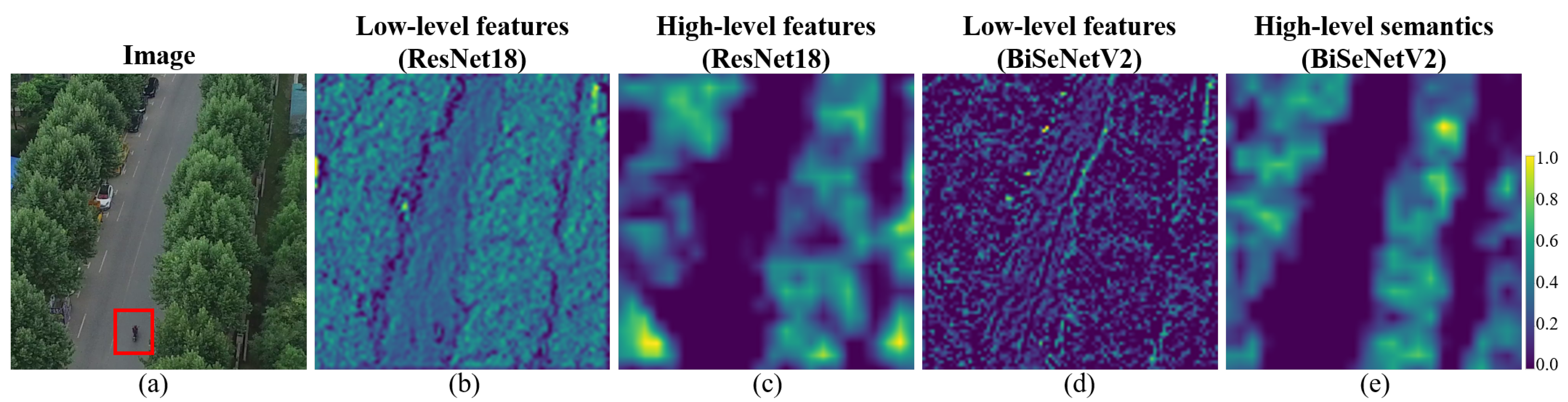
8], focus on the accumulation of contextual information over significantly large receptive fields to generate high-level semantics. The high-level semantics (Figure 2c,e) extracted using deep convolutional neural network (CNN) layers mainly depict the holistic information of the large objects and ignore small objects [9,10]. Therefore, large objects achieve high accuracy; however, small objects have extremely low accuracy.
Fortunately, the low-level features generated by the shallow layers contain small-object information, which is discovered by [9,10]. Consequently, several methods, such as the bilateral segmentation network (BiSeNet) [12], BiSeNet-v2 [13], and context aggregation network (CAgNet) [14] with dual branches, have been proposed and applied to remote sensing tasks. These methods set up a branch with shallow layers to extract low-level features that contain small-object information. The low-level features and high-level semantics extracted by the other branch are fused to make the final prediction. These methods improve the accuracy of the segmentation of small objects to some extent; however, their effects are limited. This is because the low-level features (Figure 2b,d) are the mixture of both the large and small objects. Specifically, the object details presented in Figure 2d are mainly for large objects, and we can hardly find the details for pedestrians. The low-level features extracted by shallow layers do not eliminate the predominant effects of large objects. Consequently, large objects push small objects aside when these models are trained.
Different to the dual-branch networks, a study by [15] uses a holistically nested edge detection (HED) [16] to produce closed contours with deep supervision. Semantic segmentation is obtained using SegNet [17] with the help of contours. This study achieves acceptable accuracy in the segmentation of relatively small objects (cars) in the ISPRS two-dimensional semantic labeling datasets (the Potsdam and Vaihingen datasets). However, cars are not small now in aerial images with the improvement of spatial resolution. For example, in the UAVid [4] and Aeroscapes [5] datasets, a range of objects (bikes, drones, and obstacles) that are considerably smaller than cars exist. Moreover, the contours extracted by HED exist for both large and small objects. Thus, the use of HED does not change the predominant relationship between large and small objects. Furthermore, the study in [15] uses a normalized digital surface model (nDSM) and DSM as the input of one of its model branches. However, nDSM and DSM are not always provided; thus, their application is limited.
To the best of our knowledge, the aforementioned small-object problem remains unsolved. We propose a reverse difference mechanism (RDM) to highlight small objects to address this issue. RDM can alter the predominant relationship between large and small objects. Thus, when the model is trained, small objects will not be pushed by large objects. RDM excludes large-object information from low-level features via the guidance of high-level semantics. The low-level features, which are a mixture of both large and small objects, can be the features produced by any shallow layer. The high-level semantics can be the features generated by any deep layer with large receptive fields. We design a novel neural architecture called a reverse difference network (RDNet) based on RDM. In RDNet, a detailed stream (DS) followed by RDM is proposed to obtain small-object semantics. Furthermore, a contextual stream (CS) is designed to generate high-level semantics to ensure sufficient accuracy in the segmentation of large objects. Both the small-object and high-level semantics are concatenated to make a prediction. The code of the RDNet will be available at https://github.com/yu-ni1989/RDNet, accessed on 21 July 2022. The contributions of this study are as follows.
  • A reverse difference mechanism (RDM) is proposed to highlight small objects. RDM aligns the low-level features and high-level semantics and excludes the large-object information from the low-level features via the guidance of high-level semantics. Small objects are preferentially learned during training via RDM.
  • Based on the RDM, a new semantic segmentation framework called RDNet is proposed. The RDNet significantly improves the accuracy of the segmentation of small objects. The inference speed and computational complexity of RDNet are acceptable for a resource-constrained GPU facility.
  • In RDNet, the DS and CS are designed. The DS obtains more semantics for the outputs of RDM by modeling both spatial and channel correlations. The CS, which ensures the sufficient accuracy of the segmentation of large objects, produces high-level semantics by enlarging the receptive field. Consequently, the higher accuracy scores of the segmentation of both small and large objects are achieved.

2. Related Work

Semantic segmentation can be considered as a dense prediction problem, which is first solved by a fully convolutional network (FCN) [18]. Based on the FCN framework, a wide range of semantic segmentation networks has been proposed. In this study, we categorize these semantic segmentation networks into two groups: traditional and small-object-oriented methods. Additionally, semantic segmentation networks specified in remote sensing are reviewed.

2.1. Traditional Methods

Traditional semantic segmentation networks focus on overall accuracy improvement and do not consider the scale variation issue. These methods satisfy this objective primarily by solving the lack of contextual information issues in the FCN. This is caused by local receptive fields and short-range contextual information [19]. PSPNet [7], DeepLabv3 [20], and DeepLabv3+ [21] are designed with pyramid structures to pool the feature map into multiple resolutions to enlarge receptive fields. Furthermore, connected component labeling (CCL) [22] and a dual-graph convolutional network (DGCNet) [23] satisfy the same objectives via other ways. CCL designs a novel context that contrasts local features, and DGCNet uses two orthogonal graphs to model both spatial and channel relationships. To generate dense contextual information, an attention mechanism which facilitates the modeling of long-range dependency is commonly used. Representative methods include nonlocal networks [24], CCNet [25], dual attention network (DANet) [26], expectation-maximization attention network (EMANet) [27], and squeeze-and-attention network (SANet) [28]. We do not review them in detail because they share similar self-attention mechanisms. Recently, the vision transformers (ViTs) [29] extended the attention mechanism. Then, a range of networks such as the MobileViT [30], BANet [31], and semantic segmentation by early region proxy [32] based on the transformer mechanism are proposed. The transformer-based methods have less parameters, but they consume more GPU memory and rely on powerful GPU facilities.
Furthermore, numerous networks have focused on reducing the complexity of the model and accelerating the inference speed. To meet this objective, existing studies have replaced time-consuming backbones with lightweight backbones. For example, PSPNet [7] uses ResNet50 or ResNet101 [11] as its backbone. Both the training and inference of PSPNet are time-consuming. Recent real-time semantic segmentation studies, such as BiSeNet [12] and SFNet [33], replace ResNet101 with ResNet18 and obtain a better trade-off between inference speed and accuracy. In addition to  ResNet18, recent studies have proposed a range of novel backbone networks to address real-time issues. The representative methods include MobileNet series [34,35], GhostNet [36], Xception [37], EfficientNet series [38,39], and STDC (Short-Term Dense Concatenate) [40]. Specifically, the Xception and MobileNet series use shortcut connections and depth-wise separable convolutions. The EfficientNet series use the depth-wise separable convolutions too, however, they focus on model scaling and achieve a good balance among the network depth, width, and resolution. GhostNet generates more feature maps from inexpensive operations with a series of linear transformations. STDC gradually reduces the dimensions of the feature maps and uses their aggregation for image representation. In this study, representative methods among them are tested in the experiments.

2.2. Small-Object-Oriented Methods

Recently, small-object-oriented methods, such as the gated fully fusion network (GFFNet) [6], have been introduced in several studies. GFFNet improves the accuracy of segmenting small/thin objects using a gated fully fusion (GFF) module to fuse multiple-level features. Then, multiple-level features can contribute to the segmentation simultaneously. Similar to GFFNet, SFNet [33] fuses the multiple-level features using an optical flow idea. It proposes a flow alignment module (FAM) to learn semantic flow between feature maps of adjacent levels. However, GFFNet and SFNet do not change the predominant effect of the large objects. Therefore, the improvements in the segmentation of small objects are limited.
Except for GFFNet and SFNet, most methods, such as BiSeNet [12], BiSeNetV2 [13], CAgNet [14], attentive bilateral contextual networks (ABCNet) [41], and the classification with an edge [15], improve the accuracy of the segmentation of small objects by integrating object details into the convolutions. BiSeNet, BiSeNet-v2, CAgNet, and ABCNet use dual branches to extract both object details and high-level semantics. Specifically, ABCNet integrates the self-attention mechanism into the dual-branch framework, thus it is a self-attention-based method at the same time. Classification with an edge [15] employs HED [16] to extract close contours of dominant objects and make predictions with the help of nDSM and DSM. Because the method in [15] requires diverse data inputs, it is difficult to compare it with other methods.

2.3. Semantic Segmentation Networks in Remote Sensing

In the remote sensing field, the studies by [42,43] lay the foundation for semantic segmentation. Subsequently, several excellent methods are proposed [44,45]. Among these, the study by [46] proposes a set of distance maps to improve the performance of deep CNNs. The local attention-embedding network (LANet) [47], relation-augmented FCN (RA-FCN) [48], and cross-fusion net [49] further develop the attention mechanism. The study by [50] argues that existing methods lack foreground modeling and proposes a foreground-aware relation mechanism.
In terms of high-resolution aerial image datasets, Aeroscapes [5] and UAVid [4], based on unmanned aerial vehicle (UAV) images that provide complex scenes with oblique views, include a large range of small objects. Aeroscapes contain a large range of scenes that include rural landscapes, zoos, human residences, and the sea; however, scenes near urban streets are not included. The UAVid [4] dataset is published to address this issue. Coupled with the UAVid dataset in the study of [4], a multiscale-dilation net is proposed. Experiments demonstrate its superiority over existing algorithms. However, the accuracy of segmenting UAV images is relatively lower compared with that of segmenting natural images. This issue remains unsolved.

3. RDNet

The RDNet is constructed as shown in Figure 3. Figure 3 shows the neural architecture; only the RDM, DS, CS, and the loss functions are necessary to be presented in detail. For the backbone, although the experimental tests (Section 5.3) demonstrate the superior performance of ResNet18 in RDNet, we do not specify the backbone network. Any general-purpose network, such as Xception [37], MobileNetV3 [35], GhostNet [36], EfficientNetV2 [39], and STDC [40], can be integrated into RDNet, and we cannot ensure that ResNet18 achieves superior results compared with future work. The aforementioned general-purpose networks can be easily divided into four main layers ( L Y 1 , L Y 2 , L Y 3 , and L Y 4 ). If the input image patch has H × W pixels, L Y 1 , L Y 2 , L Y 3 , and  L Y 4 extract features with reduced resolutions 1 4 H × 1 4 W , 1 8 H × 1 8 W , 1 16 H × 1 16 W , and  1 32 H × 1 32 W , respectively, as shown in Figure 3. Notably, each L Y 1 , L Y 2 , L Y 3 , and  L Y 4 contains several sublayers. For example, ResNet18 has four main layers, which is well known. If we combine the convolution, batch norm, ReLU, and max-pooling operators at the beginning of ResNet18 with the first layer, the inner layers of ResNet18 can be divided into L Y 1 , L Y 2 , L Y 3 , and  L Y 4 , which produces features with reduced resolutions 1 4 H × 1 4 W , 1 8 H × 1 8 W , 1 16 H × 1 16 W , and  1 32 H × 1 32 W .
Given an input image patch I R 3 × H × W , the backbone network is performed, and a set of features are generated. We select the features f 1 b R C 1 b × 1 4 H × 1 4 W and f 2 b R C 2 b × 1 8 H × 1 8 W generated by L Y 1 and L Y 2 as the low-level features. We present the saliency maps of the features extracted by L Y 1 , L Y 2 , L Y 3 , and  L Y 4 in ResNet18 in Figure 4 to demonstrate the rationale behind the selection for low-level features. From Figure 4b,c, f 1 b and f 2 b produced by ResNet18 are the mixture of both the large and small objects. Meanwhile, f 3 b R C 3 b × 1 16 H × 1 16 W and f 4 b R C 4 b × 1 32 H × 1 32 W generated by deep layers ( L Y 3 and L Y 4 in ResNet18) mainly depict large objects (as shown in Figure 4d,e). We can hardly find the small-object information in f 3 b and f 4 b .
Subsequently, f 4 b is processed by the CS to generate high-level semantics f h R C h × 1 32 H × 1 32 W . f h and down-sampled f 1 b are placed in an RDM (denoted by RDM1). Additionally, f h and f 2 b are placed in another RDM (denoted by RDM2). Consequently, the difference features f 1 d R 2 C 1 b × 1 8 H × 1 8 W and f 2 d R 2 C 2 b × 1 8 H × 1 8 W are produced. Then, f 1 d and f 2 d are concatenated and performed by the DS to generate the small-object semantics f s R ( 2 C 1 b + 2 C 2 b ) × 1 8 H × 1 8 W . Thus, f s and f h mainly depict small and large objects, respectively. Finally, f s and f h are concatenated to obtain the final prediction P f .

3.1. RDM

The low-level features f l R C l × H l × W l (such as f 2 b in Figure 4) extracted by shallow layers are the mixture of both the large and small objects. The high-level semantics f h R C h × H h × W h generated by the deep layers primarily depict large objects (see the saliency map of f h in Figure 4). RDM attempts to exclude large objects from f l via the guidance of f h ; thus, the predominant effects of large objects are eliminated. The principle of RDM differs from the dual-branch framework and skip connection, which have some positive effects on the segmentation of small objects. However, they do not eliminate the predominant effects of large objects. Consequently, when these models are trained, large objects push small objects aside. RDM eliminates the predominant effects of large objects using the idea of alignment and difference, as shown in Figure 5. The key innovations are two-fold: (1) the reverse difference concept and (2) the semantic alignment between f l and f h .
The reverse difference concept lays the foundation for RDM. By considering the cosine alignment branch (see Figure 5) as an instance, after  f l and f h are aligned, f h is transformed into f c o s h . Subsequently, a difference map S ( f l ) S ( f c o s h ) is produced by a difference operator. Here, S ( · ) is the Sigmoid function which transforms the intensity values in f l and f c o s h into intervals from 0 to 1. Notably, the difference must subtract f c o s h from f l . Only in this manner can numerous intensity values on the positions of large objects in S ( f l ) S ( f c o s h ) be negative. Subsequently, we use the ReLU function to set all the negative values to zero. Consequently, the large-object information is washed out, and the small-object information is highlighted.
For semantic alignment between f l and f h , f h typically has more channels and lower resolutions than f l . The up-sampling and down-sampling can change the resolution but fail to change the number of channels. Even if they have the same number of channels, we cannot ensure semantic alignments between f l and f h . For example, the ith channel in f h is more likely to contain a specific category of large objects. Does the ith channel in f l contain similar information of the same categories as the ith channel in f h ? If not, how do we ensure that the reverse difference mechanism is in effect? RDM provides two alignment modules to align the semantics from different perspectives by fully modeling the relationship between f h and f l as shown in Figure 5. The aligned high-level semantics produced by the cosine and neural alignments are f c o s h and f n e u h , respectively. The difference features f d R 2 C l × H l × W l produced by RDM are computed as follows:
f c o s d = S ( f l ) S ( f c o s h ) ,
f n e u d = S ( f l ) S ( f n e u h ) ,
f d = R e L U ( C a t ( f c o s d , f n e u d ) ) ,
where C a t ( · ) denotes the concatenation. In the following sections, the details of cosine and neural alignments are presented.

3.1.1. Cosine Alignment

The cosine alignment presented in Algorithm 1 determines the relationship between f h and f l without learning from the data. It has a mathematical explanation based on cosine similarity. First, we down-sample f l as f d o w n l R C l × H h × W h , which has the same resolution as f h . Subsequently, f h R C h × H h × W h and f d o w n l are converted into vector forms along each channel such that f h R C h × N h and f d o w n l R C l × N h , where N h = H h × W h . The cosine similarity between each pair of channels in f h and f d o w n l is then computed as
s i j c o s = f d o w n l [ i ] · f h [ j ] | f d o w n l [ i ] | × | f h [ j ] | ,
where f d o w n l [ i ] and f h [ j ] are vectors that belong to the i-th and j-th channels in f d o w n l and f h , respectively. “·” is the dot product between the vectors, and “×” is the product between the scalars. After all pairs of vectors in f h and f d o w n l are performed using Equation (4), a similarity matrix M s i m R C l × C h is constructed. We do not compute the cosine similarity per element to facilitate the implementation. The matrix multiplication “*” can be used to obtain M s i m as
M s i m = N o r m ( f d o w n l ) * N o r m ( f h T ) ,
where N o r m ( · ) is the l 2 normalization for each channel in f d o w n l and f h . l 2 normalization is essential because it ensures that the matrix multiplication is equal to the cosine similarity. f h T denotes the transpose of f h .
Algorithm 1 Cosine alignment.
  • Require: The low-level features f l R C l × H l × W l and the high-level semantics f h R C h × H h × W h
  • Ensure: The aligned f h (denoted by f c o s h R C l × H l × W l )
1:
Down-sample f l as f d o w n l R C l × H h × W h .
2:
Transform f d o w n l and f h into vector forms along channels such that f h R C h × N h and f d o w n l R C l × N h .
3:
Produce the similarity matrix M s i m R C l × C h using f d o w n l and f h as Equation (5).
4:
Obtain f c o s h R C l × N h using M s i m and f h as Equation (6).
5:
Transform and up-sample f c o s h R C l × N h such that f c o s h R C l × H l × W l .
6:
return f c o s h
A Softmax function is performed along the C h dimension to render M s i m more representable. This transforms the elements in M s i m into a set of normalized weights for f h channels. Finally, M s i m and f h are multiplied as follows.
f c o s h = M s i m * f h ,
where f c o s h is the aligned f h . The multiplication * reduces the number of channels in f h such that f c o s h has the same number of channels as f l . Furthermore, using Equation (6), we can obtain an alignment effect. As shown in Figure 6, when we take the value f c o s h ( i , k ) on the i-th row and k-th column in f c o s h as an example, f c o s h ( i , k ) is computed as:
f c o s h ( i , k ) = j = 1 C h M s i m ( i , j ) × f h ( j , k ) ,
where f h ( j , k ) is the value on the j-th row and k-th column in f h , and  M s i m ( i , j ) is the value on the i-th row and j-th column in M s i m . Consequently, f c o s h ( i , k ) is a weighted average of f h ( j , k ) , j = 1 , , C h . If the j-th channel in f h is more similar to the i-th channel in f d o w n l , M s i m ( i , j ) will be larger. Therefore, the equation gives larger weights to the channels in f h that are more similar to the i-th channel in f d o w n l . As a result, the cosine alignment tries its best to meet the objective that the i-th channel in f d o w n l and the i-th channel in f c o s h containing similar large object information.
Finally, f c o s h is transformed back into the image plane and up-sampled such that f c o s h R C l × H l × W l . f c o s h is the aligned high-level semantics produced by the cosine alignment.

3.1.2. Neural Alignment

The neural alignment, which is shown in Algorithm 2, aligns the semantics between f h and f l using convolutions. Firstly, a convolution layer with 1 × 1 kernels followed by an up-sampling operator is performed to compress f h :
f r e d h = U p ( W n e u [ C h , C l , 1 × 1 ] f h ) ,
where W n e u [ C h , C l , 1 × 1 ] is the weight matrix in the convolution layer, ⊗ is the convolution, U p ( · ) is the up-sampling, and  f r e d h R C l × H l × W l is the compressed f h . Via Equation (8), f r e d h has the same number of channels as f l . Actually, W n e u [ C h , C l , 1 × 1 ] is the learnable projection bases which projects f h into the space we prefer. This procedure has an effect of semantic alignment by iteratively optimizing the projection bases during the training.
Algorithm 2 Neural alignment.
  • Require: The low-level features f l R C l × H l × W l and the high-level semantics f h R C h × H h × W h
  • Ensure: The aligned f h (denoted by f n e u h R C l × H l × W l )
1:
Project and up-sample f h as Equation (8) to generate f r e d h R C l × H l × W l .
2:
Generate the channel attention vector v a R 2 C l × 1 via average pooling using both f l and f r e d h .
3:
Transform v a into R C l × 1 and model the correlation between the channels of f l and f r e d h based on v a .
4:
Obtain f n e u h using v a as Equation (9).
5:
return f n e u h
Then, a mutual channel attention is proposed to enhance the alignment. The traditional channel attention has been used to select informative features via introducing global weights for channels of the input features [49,51]. However, the traditional channel attention is a self-attention mechanism which does not have the alignment effect between the features generated by different layers. Here, to consider both the information in f l R C l × H l × W l and f r e d h R C l × H l × W l , we concatenate f l and f r e d h together. Based on this, the average pooling layer is performed to generate a channel attention vector v a R 2 C l × 1 . Subsequently, a convolution layer with 1 × 1 kernels, a batch normalization, and a sigmoid activation are performed on v a to model the correlations of the channels in f l and f r e d h . As a result, v a is transformed as v a R C l × 1 , which can be used directly to select the information of f r e d h by an element-by-element multiplication along the C l channels. Concretely, using v a , the aligned high-level semantics f n e u h R C l × H l × W l are formulated as:
f n e u h = v a f r e d h ,
where ⊙ is the element-by-element product along the C l channels. Finally, f n e u h is the output of the neural alignment.

3.2. DS

The f d generated by RDM is the input to DS. In RDNet, two RDM components produce difference features f 1 d R 2 C 1 b × 1 8 H × 1 8 W and f 2 d R 2 C 2 b × 1 8 H × 1 8 W . f 1 d and f 2 d are concatenated as the final output f d R C d × H l × W l of the RDM components, where C d = 2 C 1 b + 2 C 2 b , H l = 1 8 H , and W l = 1 8 W . f d includes only small-object information with fewer semantics. The DS is proposed to obtain more semantics to facilitate prediction without adding excessive parameters.
The commonly used method adds several convolutional layers with strides, such as ResNet18 to generate semantics. This method significantly increases the number of parameters and computational complexity. Here, we use depth-wise convolution to address these issues. Furthermore, when the stride is set to two or larger, the convolution enlarges the receptive field; however, some extremely small objects, such as pedestrians in UAVid, are ignored. Therefore, we do not use any strides. Additionally, we do not know which kernel size is most suitable. A larger kernel size suppresses small objects, whereas a smaller kernel size generates less semantic information. Here, the DS designs two convolutional branches using 1 × 1 and 3 × 3 kernels to alleviate the negative effects produced by a fixed kernel size, as shown in Figure 7.
The first branch contains only a single convolutional layer with 1 × 1 kernels and is simple and lightweight. It convolves f d using a small kernel size and creates a correlation between all the channels. We use f 1 × 1 d R C d × H l × W l to denote the output of the first branch. The second branch convolves f d using a larger kernel size. It makes spatial correlations using a depth-wise convolution with 3 × 3 kernels and makes a cross-channel correlation using shared kernels. Specifically, f d is first processed using a depth-wise convolutional layer to obtain a spatially correlated feature map f s p R C d × H l × W l . Subsequently, a cross-channel correlation is performed. This adaptively pools f s p into feature vector v s p R C d × 1 . A two-dimensional convolutional layer with padding and 3 × 3 kernels, followed by sigmoid activation, is then used to make correlations along the channels:
v c c = S ( W c [ 2 C l , 2 C l , 3 × 3 ] P ( v s p ) ) ,
where v c c R C d × 1 is the derived cross-channel correlated feature vector, P ( · ) is padding, S ( · ) is sigmoid activation, and W c [ 2 C l , 2 C l , 3 × 3 ] is the weight matrix of the convolution. Subsequently, the features f 3 × 3 d R C d × H l × W l extracted by the second branch are:
f 3 × 3 d = f s p E x p a n d ( v c c ) ,
where “•” is the element-by-element product of the image plane. The activated v c c is expanded to the same dimension as f s p by an expanding operator E x p a n d ( · ) to perform multiplication.
After both branches are performed, the small-object semantics f s R C d × H l × W l that fully depict small objects are generated as follows.
f s = R e L U ( f 1 × 1 d + f 3 × 3 d ) ,
where “+” is element-by-element addition.

3.3. CS

The CS is designed to process the output f 4 b R C b × 1 32 H × 1 32 W of L Y 4 in the backbone network. Here, we generate high-level semantics f h by extending the receptive field. This compels f h to further focus on large objects. The average pooling pyramid (APP) [7] is utilized to enlarge the receptive field. Unlike the strategy that directly enlarges the kernel size, APP does not increase the computational complexity [7]. As shown in Figure 8, the APP of the CS pools f 4 b into three layers with different down-sampled resolutions: 11 × 11 1 64 H × 1 64 W , 8 × 8 , and 5 × 5 .
Although the receptive field is enlarged, it is difficult to generate continuous contextual information that washes out heterogeneity in large-object features. Dual attention [26] is used to fully model long-range dependencies to address this issue. Dual attention, which includes a position attention module (PAM) and channel attention module (CAM), considers both spatial and channel information. The PAM computes the self-attention map for each position on the feature-image plane, and the CAM computes the self-attention map along the channels. They share similar procedures, which are detailed in [26], for producing these self-attention maps using matrix multiplication. Then, the input features are enhanced by these self-attention maps. Thus, the enhanced features produced by PAM and CAM contain continuous spatial dependency and channel dependency information, respectively.
In the i-th layer of Figure 8, f 4 b is averagely pooled as the down-sampled feature f i c s R C b × H i × W i . Two reduced feature maps f ¯ i c s R C r × H i × W i and f ˜ i c s R C r × H i × W i are first generated by two convolutions with 1 × 1 kernels based on f i c s . Here, C r is set to C b / 12 . f ¯ i c s is processed by the PAM to obtain continuous spatial dependence information. Subsequently, a depth-wise convolutional layer with 3 × 3 kernels is used to generate the semantics f ¯ i s e m R C r × H i × W i . f ˜ i c s is processed by CAM to obtain dependence information along the channels. Again, a depth-wise convolutional layer with 3 × 3 kernels is used to generate the semantics f ˜ i s e m R C r × H i × W i .
After all of the layers are performed, a set of f ¯ i s e m and f ˜ i s e m , i = 1 3 are obtained. All f ¯ i s e m and f ˜ i s e m , i = 1 3 are up-sampled to the same resolution as f 4 b and concatenated with f 4 b . Subsequently, the high-level semantics f h R C b × 1 32 H × 1 32 W are obtained by a convolution with 1 × 1 kernels.

3.4. The Loss Function

As shown in Figure 3, the loss function L is composed of two terms:
L = L m a i n ( T , P f ) + L a u x ( T , P a ) ,
where L m a i n ( T , P f ) is the selected main loss which penalizes the errors in the final prediction, P f . L a u x ( T , P a ) is the auxiliary loss which penalizes the errors in the auxiliary prediction P a produced by the high-level semantics f h . P f and P a are produced using similar prediction layers. First, the prediction layer convolves the input features using 3 × 3 kernels. Subsequently, batch normalization and ReLU activation are performed. Finally, the prediction is produced using a convolutional layer with 1 × 1 kernels. The differences between the prediction layers for P f and P a are only the parameters for the two inner convolutions. For P f , we set the input and output numbers of the channels of the first convolution as C b + 2 C 1 b + 2 C 2 b and 128, where C 1 b , C 2 b and C b are the number of channels for the small-object semantics f 1 s and f 2 s and the high-level semantics f h , respectively. The input and output numbers of the channels of the remaining convolution are set to 128 and K, where K is the number of classes. For P a , the input and output numbers of the channels for the first convolution are set to C b and 64, respectively, and the input and output numbers of the channels for the remaining convolution are set to 64 and K.
We integrate a threshold T r L with the standard cross-entropy loss to further highlight small objects without adding prior information about the data using L m a i n ( T , P f ) . For more detail, we compute the individual main loss L m a i n ( T , P f ) [ i ] of each pixel in P f as follows:
L m a i n ( T , P f ) [ i ] = P f ( i ) [ T ( i ) ] + l o g ( j = 1 K e P f ( i ) [ j ] ) ,
where T ( i ) is the ground-truth label of the i-th pixel and K is the number of categories. P f ( i ) is the i-th vector in P f containing probabilistic values belonging to all categories of the i-th pixel. P f ( i ) [ j ] is the probability that the i-th pixel belongs to the j-th category. Then, an indicator function I is defined as
I [ i ] = 1 , L m a i n ( T , P f ) [ i ] T r L , 0 , L m a i n ( T , P f ) [ i ] < T r L .
where I [ i ] is the indicator of the i-th pixel in the input image I, and T r L = 0.7 . L m a i n ( T , P f ) is computed based on I and L m a i n ( T , P f ) [ i ] as follows:
L m a i n ( T , P f ) = i = 1 N I [ i ] × L m a i n ( T , P f ) [ i ] i = 1 N I [ i ] ,
where N denotes the number of pixels in I. CNN-based models are advantageous for the recognition of large objects and elimination of heterogeneity in large objects. After several training iterations, the losses in the prediction of large objects will be smaller than those of small objects. Larger losses are more likely to occur on pixels in small objects. Therefore, apart from the RDM, L m a i n ( T , P f ) further highlights the small objects during the backward procedure to some extent.
L a u x ( T , P a ) uses the standard cross-entropy loss function without changing the optimization preference for large (dominant) objects. Thus, L a u x ( T , P a ) favors the preference of f h for depicting large objects, which ensures the accuracy of large-object recognition. L a u x ( T , P a ) is formulated as
L a u x ( T , P a ) = i = 1 N P a ( i ) [ T ( i ) ] + l o g ( j = 1 K e P a ( i ) [ j ] ) N .

4. Datasets

In this paper, the UAVid and Aeroscapes datasets are employed to evaluate the performance in the segmentation of small objects. Both the two datasets contain objects having large-scale variations. It is notable that we do not employ the ISPRS Potsdam and Vaihingen datasets. As discussed in Section 1, only cars contained in the Potsdam and Vaihingen datasets are smaller. However, now, cars in UAV images are not small, and a large range of objects are much smaller than cars.

4.1. The UAVid Benchmark

The UAVid benchmark [4] is a newly published dataset of aerial imagery. Its detailed information is given on its official website (https://uavid.nl/ (accessed on 1 May 2020)). UAVid contains 8 classes, defined as “Clutter”, “Building”, “Road”, “Tree”, “Vegetation”, “Moving car”, “Static car”, and “Human”. UAVid focuses on the scenes near streets but consists of diverse landscapes including downtown areas (Figure 9a), villa areas (Figure 9b), and outskirts (Figure 9c). For the scale variations, to accurately measure the size, we calculate the average number of pixels for a single object in each category in Table 1. To simplify the notation, we use “Build.”, “Veg.”, “Mov.c.”, and “Stat.c.” to denote the Building, Vegetation, Moving car, and Static car classes. Definitely, the instances in the Human class have the smallest size (555.0 pixels) on average. More importantly, our objective is for the recognition of footpath-level objects. It is notable that here it is “footpath”, not “road” or “street”. Footpaths are much narrower than roads or streets. In UAVid, only the Human class contains the footpath-level objects. Therefore, we only consider that the Human class has such a small size. In addition, although cars are much larger than pedestrians, they are not as large as the other objects. Therefore, we consider that the Stat.c and Mov.c classes have medium sizes. In this way, the existing categories are divided into three groups, as shown in Table 1.

4.2. The Aeroscapes Benchmark

The Aeroscapes [5] benchmark is another aerial dataset annotated for dense semantic segmentations. The details of Aeroscapes are shown on its official website (https://github.com/ishann/aeroscapes (accessed on 29 May 2020)). As shown in Figure 10, Aeroscapes contains a large range of scenes, including countryside, playgrounds, farmlands, roads, animal zoos, human settlements, and seascapes, among others. There are 12 classes that are defined as: “Background”, “Person”, “Bike”, “Car”, “Drone”, “Boat”, “Animal”, “Obstacle”, “Construction”, “Vegetation”, “Road”, and “Sky”. For brevity, we use “b.g.”, “Constr.”, and “Veg.” as the simplified notations for the “Background”, “Construction”, and “Vegetation” classes, respectively. Among these categories, the Person, Bike, Drone, Obstacle, and Animal classes contain footpath-level objects from a human perspective. As we all know, the UAV platform is oblique and the flight altitude is variable. For some specific scenes, the spatial resolutions of the images obtained by the UAV platform are really high. In this case, the footpath-level objects may not be small. To eliminate the larger ones caused by the UAV platform among the footpath-level objects, we calculate the average number of pixels for a single object in each category in Table 2. In Table 2, the oblique view and flight altitude do not enlarge the sizes of instances in the Person, Bike, Drone, and Obstacle classes. Therefore, we consider that the Person, Bike, Drone, and Obstacle classes have small sizes. However, the Animal class is influenced. The animal zoo scene is relatively smaller than the other scenes. When the UAV platform collects data, it must be nearer to the targets. This leads to really high spatial resolutions, and thus the animals in the image are not small (see Figure 10f). Therefore, we consider that the Animal class has medium sizes. In detail, the existing categories in Aeroscapes are divided into three groups, as shown Table 2.

5. Experiments

Firstly, we introduce the evaluation metrics used in this study and the implementation details of the training procedure. Subsequently, the experimental settings are discussed. Then, the results of RDNet and the comparisons with existing methods for both the UAVid and Aeroscapes datasets are presented. Finally, we discuss some issues of interest.

5.1. Evaluation Metrics

To keep consistency with existing public evaluations, such as the studies by [4,5,14], we mainly use the IoU scores as the evaluation metrics. For the dataset having a range of classes with small/medium/large objects that pose a challenge to analyze the performance across scales, we divide the existing classes into small, medium, and large groups based on the scale information presented in Table 1 and Table 2. Accordingly, the mean IoU score of the classes in each group is computed. Thus, three mean IoU scores m I o U s , m I o U m , and m I o U l are defined for the small, medium, and large groups, respectively. As these metrics are well-known and easily understood, we do not present them in any detail here.

5.2. Implementation Details

The proposed RDNet is implemented based on Pytorch. To train the network, we use stochastic gradient descent as the optimizer. The commonly used learning rate policy is employed, where the initial learning rate is multiplied by ( 1 i t e r m a x _ i t e r ) p o w e r for each iteration. Here, p o w e r and the initial learning rate are set to 0.9 and 10 4 , respectively. We train the RDNet on the training set for 10 epochs. In each epoch, we randomly selected 30,000 image patches with a batch size of three. Each patch is 704 × 704 in size. In more detail, to randomly select each image patch, we randomly generate two values h r and w r to indicate the top-left corner. Then, the image patch is copied from the original image based on the coordinates ( h r , w r ) and ( h r + 704 , w r + 704 ) . Both the RDNet models for UAVid and Aeroscapes are trained using these settings. As is known, the training procedure usually trains the model iteratively. For each iteration, we actually obtain a trained model. As we focus on the small objects, we use the trained model that gives the highest accuracy scores for the small objects to obtain the final segmentation results. In terms of the comparison methods, we obtain the trained model for testing in the same way.

5.3. Experimental Settings Based on Validation

5.3.1. The Backbone Selection

Currently, there are a large range of general-purpose networks which can be used as the backbone. Our objective is to select a backbone which can make a good trade-off between computational complexity and accuracy. We list the integrations of RDNet with the representative general-purpose networks which have the real-time property in Table 3. MobileNetV3, GhostNet, STDC, EfficientNetV2, Xception, and ResNet18, which are commonly used CNN-based networks, can be integrated into RDNet in the way shown in Figure 3. MobileViT is a new general-purpose network that combines the strengths of CNNs and ViTs [29]. Although the architecture of MobileViT is different with the purely CNN-based networks, it can easily integrate with the RDNet framework. At the beginning of the MobileViT, a MobileNetV2 [34] block sequence is used to extract a set of low-level features. Subsequently, these low-level features are put into the ViT sequence to generate high-level semantics. We select the low-level feature maps with 1 4 H × 1 4 W and 1 8 H × 1 8 W pixels as the f 1 b and f 2 b and select the high-level semantics produced by the ViT sequence as the f h . Then, the RDNet based on MobileViT can be constructed using the way shown in Figure 3.
In Table 3, the number of parameters (Pars.), computation complexity, GPU memory consumption (Mem.), and mIoU scores are presented. The computation complexity is measured by the float-point operations (FLOPs) and frames per second (FPS), which are computed using an image patch with 3 × 1536 × 1536 pixels. The accuracy scores are obtained in the validation set of UAVid. Notably, the validation set is not used for training the model. RDNet(ResNet18), which is the RDNet version using ResNet18 as backbone, obtains the highest accuracy. RDNet(Xception) and RDNet(EfficientNetV2) obtain really close accuracy to RDNet(ResNet18), however, they cannot surpass RDNet(ResNet18). Xception and EfficientNetV2 are constructed based on the depth-wise separable convolutions, which reduces many weights for cross-channel modeling. In contrast, ResNet18 fully models the cross-channel relationship using full convolutional operators. This suggests that the cross-channel modeling in the backbone is beneficial to RDNet. The RDNet(MobileViT) has the potential for accuracy improvements because it contains only 2.08M parameters. Unfortunately, the GPU memory consumption of RDNet(MobileViT) is really huge (28.5G), which limits its application. The RDNet(MobileNetV3) and RDNet(GhostNet) are lightweight and fast. However, they achieve much lower accuracy than the RDNet(ResNet18). From the comparison, the RDNet(ResNet18) obtains better trade-off among parameters, complexity, speed, GPU memory consumption, and accuracy. Therefore, we select the ResNet18 as the default backbone.

5.3.2. The Selection of Comparison Methods

As of now, there are hundreds of networks for semantic segmentation tasks, and we cannot compare all these methods with our RDNet. As our RDNet focuses on small objects, we test the existing small-object-oriented methods for which official codes have been released. They are BiSeNet, ABCNet, SFNet, BiSeNetV2, and GFFNet, which were introduced in Section 2.2. Notably, there exists a large range of backbone networks; we cannot test all the backbones for each method. Here, we use the backbone provided by the official codes of each method. Table 3 shows the properties and accuracies of these methods. We can find that most of the small-object-oriented methods have real-time property and prefer ResNet18. In addition, we select three representative networks from traditional methods (see Section 2.1). The DANet [26] is one of the self-attention-based methods, and the DeepLabV3 [21] is one of the methods using atrous convolutions and pyramids. MobileViT [30] is the representative method using vision transformer [29]. For the semantic segmentation task, MobileViT [30] uses the DeepLabV3 architecture and replaces the ResNet101.
In Table 3, DANet and DeepLabV3, can only achieve higher m I o U scores than BiSeNet when they use ResNet101. In most cases, they receive lower accuracy scores than the small-object-oriented methods, though they use much more complex backbones (ResNet101) as default. More importantly, based on the m I o U s scores, the performance for segmenting small objects is more inferior. Although MobileViT achieves a relatively higher m I o U s score of segmenting small objects than DANet and DeepLabV3, it still cannot surpass the existing small-object-oriented methods. Furthermore, the GPU memory consumption of MobileViT is huge (27.8G). Therefore, we pay attention mainly to the comparison between RDNet and small-object-oriented methods in more detail in the following. Meanwhile, to fully compare RDNet to the state of the art, we show the published results for each dataset.

5.4. Results on UAVid

This section is divided into two parts: the quantitative and visual results. The details of the UAVid dataset are presented in Section 4.1. Specifically, the human class has small sizes.

5.4.1. Quantitative Results

Table 4 shows the quantitative results for the UAVid test set. In Table 4, the comparisons are divided into two groups. The first group shows state-of-the-art results obtained by MSD [4], CAgNet [14], ABCNet [41], and BANet [31]. MSD, CAgNet, ABCNet, and BANet officially publish their results on UAVid. We directly quote their accuracy scores here. The second group shows the accuracy scores obtained by the small-object-oriented methods that are not included in state-of-the-art results. It shows the results obtained by BiSeNet [12], GFFNet [6], SFNet [33], and BiSeNetV2 [13]. We trained BiSeNet, GFFNet, SFNet, and BiSeNetV2 ourselves and used the official server (https://uavid.nl/, accessed on 1 May 2020) of UAVid to obtain the accuracy scores.
In Table 4, RDNet obtains the highest mIoU score across these methods. More importantly, for each of the small, medium, and large groups, our RDNet obtains the highest accuracy (which is denoted by the m I o U s , m I o U m and m I o U l scores). This means that the performance of segmenting large and medium objects does not become worse when our RDNet improves the accuracy of segmenting small objects. On the contrary, the accuracy scores ( m I o U m and m I o U l ) of segmenting the medium and large objects are further improved. For the segmentation of small objects, our RDNet achieves 4.5–18.9% higher m I o U s scores than the existing methods. Notably, BiSeNetV2, GFFNet, and SFNet, which are powerful small-object-oriented methods, already have great performance in segmenting small objects, as noted in the introduction in Section 2.2. Therefore, our RDNet, which obtains higher m I o U s than BiSeNetV2, GFFNet, and SFNet, has a stronger ability for segmenting small objects. Moreover, compared with state-of-the-art results, our RDNet achieves 11.8–18.9% higher m I o U s scores, which is a significant improvement. Therefore, based on the results in Table 4, the superiority of our RDNet, especially for the segmentation of small objects, is validated.

5.4.2. Visual Results

To facilitate the visual comparison, we use the prediction maps of the validation set which has the ground-truth. Notably, the validation set is not used for training. Figure 11 shows the visual results for all classes in UAVid. Notably, we do not present the scenes that do not satisfy the scale-variation issue. Furthermore, SFNet and BiSeNetV2 achieve higher mIoU and m I o U s scores than the other existing methods, as shown in Table 4; therefore, we only visually compare the results of RDNet with those of SFNet and BiSeNetV2 owing to the page limits. Based on the ground-truth (Figure 11, second column), RDNet provides more reliable results compared with other methods. The small objects extracted by RDNet are more complete, and the segmented large and medium objects are better.
In terms of small objects, we highlight the subareas that challenge the segmentation of small objects in the first and second images (Figure 11, first and second rows) using red rectangles. The sanitation worker in the first image and the man near a car in the second image are combined with a particularly complex background. The pedestrians in the second image have similar spectral features to the shadow of the buildings. Consequently, both SFNet and BiSeNet-v2 miss these small targets in the results, whereas RDNet identifies all of them (Figure 11, last column). In terms of large objects, we highlight the subareas that challenge the segmentation of large objects in the second and third images (Figure 11, second and last rows) using black rectangles. In the second image, the subarea contains trees, vegetation, and roads. These are different types of large objects shading each other, which results in difficulty of recognition. Neither SFNet nor BiSeNet-v2 segments this subarea well, whereas RDNet succeeds. In the last image, the subarea contains a building surrounded by vegetation. BiSeNet-v2 and RDNet misclassify the building, whereas RDNet produces a perfect result.
The visual results show that RDNet obtains superior results for both the small and large objects in UAVid. The accuracy of segmenting large objects is not reduced when RDNet highlights the small objects. On the contrary, the accuracy of segmenting large objects is further improved.

5.5. Results on Aeroscapes

The structure of the results on the Aeroscapes dataset is similar to Section 5.4. The details of the Aeroscapes dataset are presented in Section 4.2. Specifically, the person, bike, drone, and obstacle classes have small sizes.

5.5.1. Quantitative Results

We compare the results of RDNet with the state-of-the-art results specified in Aeroscapes and those obtained using BiSeNet, ABCNet, GFFNet, SFNet, and BiSeNetV2. The accuracy values are presented in Table 5. In terms of the state-of-the-art results, that is, EKT-Ensemble [5], specific issues must be recognized. In addition to the precise mIoU scores, the evaluation for IoU scores is only provided in a bar chart with an accuracy axis (see details in [5]). We cite this evaluation by carefully determining the values along the accuracy axis. Therefore, these values are considered approximate (≈) in Table 5. [5] assembled different datasets, including PASCAL [52], CityScapes [53], ADE20k [54], and ImageNet [55] to improve accuracy, owing to the large range of scenes contained in Aeroscapes. The results using this assembly, denoted as EKT-Ensemble, achieve a 57.1% mIoU score.
As shown in Table 5, RDNet obtains the highest mIoU score among all the methods. More importantly, the m I o U s score for segmenting small objects, m I o U m score for segmenting medium objects, and m I o U l score for segmenting large objects obtained by RDNet are all higher than those obtained by the other methods. This validates that RDNet further improves accuracy for the segmentation of large objects when it improves the accuracy of segmenting small objects. Specifically, the m I o U s score is 3.9% higher than that of BiSeNetV2, which ranks the second. For the bike class with the smallest objects, our RDNet obtains at least a 7.8% higher IoU score than the other methods. For the person class with small objects, RDNet obtains at least 5.0% higher accuracy than the other methods. SFNet obtains a higher IoU score for segmenting the obstacle class with small objects. This validates that SFNet has great power for segmenting small objects. However, compared with our RDNet, SFNet obtains lower IoU scores for segmenting the other classes with small objects, including the person, bike, and drone classes. This validates the superiority of RDNet.

5.5.2. Visual Results

Aeroscapes contains numerous scenes with large-scale variations between the classes. Here, we select four images that cover the classes with small objects and the objects challenging the segmentation in Figure 12. From these visual results, we observe some mistakes in each of the predictions, which demonstrates the challenges of the Aeroscapes dataset. RDNet obtains reasonable segmentation results, in which all objects are recognized. Compared with SFNet and BiSeNet-v2, RDNet obtains superior results with less misclassification in each image. Specifically, the first row of Figure 12 presents the smallest object, a bike. The result obtained by RDNet are much better than those obtained by SFNet and BiSeNetV2. In the second row of Figure 12, RDNet obtains superior results for the segmentation of the person and drone classes. In Table 5, SFNet obtains a higher IoU score for segmenting obstacles than RDNet. However, in the visual results, RDNet can achieve better segmentation results in a range of scenes, such as the third row in Figure 12. In the last row of Figure 12, we show the segmentation results of the animal class. RDNet obtains the best results for segmenting animals in the image.

6. Discussion

6.1. Ablation Study

In RDNet, we propose three modules, including RDM, DS, and CS. RDM has two alignment branches: cosine alignment ( R D M C ) and neural alignment ( R D M N ). Here, we analyze the influence of each of these factors. We compare the results obtained by RDNet without each component with those of the complete RDNet to directly demonstrate the effects. We use RDNet-RDM as the simplified form of the RDNet without the RDM. The other variants of RDNet are denoted in similar forms.
Table 6 shows the ablation study using the Aeroscapes dataset. RDNet-RDM shows the lowest accuracy. Compared with RDNet, the mIoU score decreases by more than 6%. Moreover, the m I o U s score of RDNet-RDM is only 31.9% which is considerably lower than those of the RDNet and other variants. This demonstrates that RDM has a significant influence on improving accuracy scores of segmenting small objects. DS has positive roles for segmenting small and medium objects based on the changes in the m I o U s and m I o U m scores. CS generates high-level semantics which primarily depict large objects. From Table 6, CS satisfies the objective. When the CS is removed, the high-level semantics become f 4 b produced by the deepest layer ( L Y 4 ) in ResNet18, and the m I o U l score for the segmentation of large objects decreases. R D M C and R D M N are the inner parts of RDM. Based on the m I o U s scores, each of these has a positive influence on the segmentation of small objects. After they are combined as RDM, the accuracy of the segmentation of small objects increases significantly.
When CS and DS are both removed from RDNet, the network only contains ResNet18 and RDM, which is shown in the second row in Table 6. The high-level semantics f h in ResNet18+RDM are the output of L Y 4 in ResNet18 directly. ResNet18+RDM is really simple, its FLOPs score is 70G less than that of BiSeNetV2. The m I o U s score of segmenting small objects obtained by ResNet18+RDM can meet 40.7%, which is 2.4% higher than that obtained by BiSeNetV2. As shown in Table 5, BiSeNetV2 obtains a m I o U s score of segmenting small objects 3.9% lower than our RDNet, however, it obtains a m I o U s score higher than the other existing methods. In other words, just using RDM and the simple backbone ResNet18, a higher accuracy of segmenting small objects than other existing methods can be obtained. This validates the great power of RDM for segmenting small objects again.

6.2. The Output of Each Module in RDNet

As shown in Figure 2, the high-level semantics extracted by deep layers primarily depict large objects. The low-level features are a mixture of the large and small objects. Although small-object information is recorded in the low-level features, large-object information plays a dominant role. This is why the existing deep-learning-based methods obtain high accuracy for segmenting large objects, while achieving low accuracy for segmenting small objects (see Table 4).
To fully analyze the positive influences of each module in RDNet, we present the saliency map of the features produced by each module in Figure 13. The features f 1 b and f 2 b generated by the L Y 1 and L Y 2 in ResNet18 have the same properties as the low-level features in Figure 2. The high-level semantics f h extracted by CS and f 4 b generated by the deep layer L Y 4 in ResNet18 have the same properties as the high-level semantics presented in Figure 2. However, from the comparison between f 4 b and f h in Figure 13, the contextual information in f h is more homogeneous, which facilitates the representation of large objects. This validates the positive effect of the CS from a visual perspective.
In Figure 13, the difference features f 1 d and f 2 d produced by the proposed RDM fully highlight small objects and exclude the predominant effect of large objects. This proves that RDM meets the objective of changing the predominant relationship between large and small objects. However, f 1 d and f 2 d only locate the small objects; they cannot depict the small objects well. A DS is proposed to generate more semantics to address this issue. After the DS is performed using f 1 d and f 2 d as its input, the generated small-object semantics f s contain the necessary semantics for depicting more properties of a small object. Coupled with the quantitative analysis in Table 6, we can conclude that RDM, DS, and CS are essential for RDNet, specifically RDM, which plays a vital role in improving the representation ability of small objects.

6.3. The Usage of Complex Backbones

In Section 5.3.1, we select ResNet18 to make a good trade-off between computational complexity and accuracy. Here, we give a discussion for the usage of more complex backbones via the segmentation in Aeroscapes. In Table 7, ResNet50 and ResNet101 are integrated. For comparison, the small-object-oriented methods that use backbone networks are tested. In terms of the small-object-oriented methods, including BiSeNet, ABCNet, GFFNet, and SFNet, the complex backbones cannot improve the m I o U s score for segmenting small objects. However, the m I o U m and m I o U l scores improve compared with those in Table 5 to some extent. The main reason is that they do not change the predominant effects of large objects. For our RDNet, the complex backbones improve not only the m I o U m and m I o U l scores for segmenting medium and large objects but also the m I o U s score for segmenting small objects.
In Table 7, RDNet obtains the highest m I o U s , m I o U m , and m I o U l scores. Specifically, when ResNet50 is used, RDNet achieves a 7.4% higher m I o U s score for segmenting small objects than SFNet, which ranks second. For the usage of ResNet101, RDNet obtains a 7.9% higher m I o U s score than SFNet. To conclude, the usage of complex backbones cannot alter the superiority of RDNet.

7. Conclusions

In this study, a novel semantic segmentation network called RDNet is proposed for aerial imagery. In RDNet, RDM is first proposed to highlight small objects. RDM develops a reverse difference concept and aligns the semantics for both high-level and low-level features. Consequently, RDM eliminates the predominant effect of large objects in the low-level features. Then, the DS, which models the spatial and cross-channel correlations, is proposed to generate small-object semantics using the output of RDM. Additionally, the CS is designed using an average pooling pyramid and dual attention to generate high-level semantics. Finally, the small-object semantics bearing the small objects and high-level semantics that focus on the large objects are combined to make a prediction.
Two aerial datasets are used to fully analyze the performance of RDNet: UAVid and Aeroscapes. Based on the experimental results, RDNet obtains superior results compared with the existing methods for both datasets. The accuracy scores of segmenting small, medium, and large objects are all improved. More importantly, the accuracy improvement for segmenting small objects is prominent. According to Table 3, RDNet has less computational complexity and uses less GPU memory compared with the existing small-object-oriented methods. This shows that RDNet achieves superior results using less computing resources. The ablation study demonstrates that the proposed RDM plays a vital role in the accuracy improvement of the segmentation of small objects. The DS further enhances the output of RDM, and the CS ensures good performance in segmenting large objects. Meanwhile, based on the visualization of the output, the positive effect of each module in RDNet is vividly shown.
In the future, the resolution of remote sensing images will be further improved, though the current resolution is so high that footpath-level objects are recorded well. Small object recognition will become more important. RDNet architecture, which highlights small objects for deep-leaning-based models, will be used for more applications in the field of remote sensing.

Author Contributions

Methodology, software, validation, writing—original draft preparation, Huan Ni; supervision, resources, investigation, writing—review and editing, Jocelyn Chanussot; methodology, investigation, resources, funding acquisition, Xiaonan Niu; investigation, writing—review and editing, Hong Tang and Haiyan Guan. All authors have read and agreed to the published version of the manuscript.

Funding

National Natural Science Foundation of China (Grant No. 41901310, 41971414, and 41801384).

Data Availability Statement

Not applicable.

Conflicts of Interest

The authors declare no conflict of interest.

References

  1. Han, W.; Chen, J.; Wang, L.; Feng, R.; Li, F.; Wu, L.; Tian, T.; Yan, J. Methods for Small, Weak Object Detection in Optical High-Resolution Remote Sensing Images: A survey of advances and challenges. IEEE Geosci. Remote Sens. Mag. 2021, 9, 8–34. [Google Scholar] [CrossRef]
  2. Chen, Z.; Gong, Z.; Yang, S.; Ma, Q.; Kan, C. Impact of extreme weather events on urban human flow: A perspective from location-based service data. Comput. Environ. Urban Syst. 2020, 83, 101520. [Google Scholar] [CrossRef] [PubMed]
  3. Castellano, G.; Castiello, C.; Mencar, C.; Vessio, G. Crowd Detection in Aerial Images Using Spatial Graphs and Fully-Convolutional Neural Networks. IEEE Access 2020, 8, 64534–64544. [Google Scholar] [CrossRef]
  4. Lyu, Y.; Vosselman, G.; Xia, G.S.; Yilmaz, A.; Yang, M.Y. UAVid: A semantic segmentation dataset for UAV imagery. ISPRS J. Photogramm. Remote Sens. 2020, 165, 108–119. [Google Scholar] [CrossRef]
  5. Nigam, I.; Huang, C.; Ramanan, D. Ensemble Knowledge Transfer for Semantic Segmentation. In Proceedings of the 2018 IEEE Winter Conference on Applications of Computer Vision (WACV), Lake Tahoe, NV, USA, 12–15 March 2018; pp. 1499–1508. [Google Scholar] [CrossRef]
  6. Li, X.; Zhao, H.; Han, L.; Tong, Y.; Tan, S.; Yang, K. Gated Fully Fusion for Semantic Segmentation. Proc. AAAI Conf. Artif. Intell. 2020, 34, 11418–11425. [Google Scholar] [CrossRef]
  7. Zhao, H.; Shi, J.; Qi, X.; Wang, X.; Jia, J. Pyramid Scene Parsing Network. In Proceedings of the 2017 IEEE/CVF Conference on Computer Vision and Pattern Recognition (CVPR), Honolulu, HI, USA, 21–26 July 2017; pp. 6230–6239. [Google Scholar] [CrossRef]
  8. Zhao, H.; Zhang, Y.; Liu, S.; Shi, J.; Loy, C.C.; Lin, D.; Jia, J. PSANet: Point-wise Spatial Attention Network for Scene Parsing. In Proceedings of the Computer Vision—ECCV, Munich, Germany, 8–14 September 2018; Ferrari, V., Hebert, M., Sminchisescu, C., Weiss, Y., Eds.; Springer International Publishing: Cham, Switzerland, 2018; pp. 270–286. [Google Scholar]
  9. Lin, T.; Dollár, P.; Girshick, R.; He, K.; Hariharan, B.; Belongie, S. Feature Pyramid Networks for Object Detection. In Proceedings of the 2017 IEEE/CVF Conference on Computer Vision and Pattern Recognition (CVPR), Honolulu, HI, USA, 21–26 July 2017; pp. 936–944. [Google Scholar] [CrossRef]
  10. Tian, Z.; Zhao, H.; Shu, M.; Yang, Z.; Li, R.; Jia, J. Prior Guided Feature Enrichment Network for Few-Shot Segmentation. IEEE Trans. Pattern Anal. Mach. Intell. 2020. early access. [Google Scholar] [CrossRef]
  11. He, K.; Zhang, X.; Ren, S.; Sun, J. Deep Residual Learning for Image Recognition. In Proceedings of the 2016 IEEE/CVF Conference on Computer Vision and Pattern Recognition (CVPR), Las Vegas, NV, USA, 26 June–1 July 2016; pp. 770–778. [Google Scholar] [CrossRef] [Green Version]
  12. Yu, C.; Wang, J.; Peng, C.; Gao, C.; Yu, G.; Sang, N. BiSeNet: Bilateral Segmentation Network for Real-Time Semantic Segmentation. In Proceedings of the Computer Vision—ECCV, Munich, Germany, 8–14 September 2018; Ferrari, V., Hebert, M., Sminchisescu, C., Weiss, Y., Eds.; Springer International Publishing: Cham, Switzerland, 2018; pp. 334–349. [Google Scholar]
  13. Yu, C.; Gao, C.; Wang, J.; Yu, G.; Shen, C.; Sang, N. BiSeNet V2: Bilateral Network with Guided Aggregation for Real-Time Semantic Segmentation. Int. J. Comput. Vis. 2021, 129, 3051–3068. [Google Scholar] [CrossRef]
  14. Yang, M.Y.; Kumaar, S.; Lyu, Y.; Nex, F. Real-time Semantic Segmentation with Context Aggregation Network. ISPRS J. Photogramm. Remote Sens. 2021, 178, 124–134. [Google Scholar] [CrossRef]
  15. Marmanis, D.; Schindler, K.; Wegner, J.; Galliani, S.; Datcu, M.; Stilla, U. Classification with an edge: Improving semantic image segmentation with boundary detection. ISPRS J. Photogramm. Remote Sens. 2018, 135, 158–172. [Google Scholar] [CrossRef]
  16. Xie, S.; Tu, Z. Holistically-Nested Edge Detection. In Proceedings of the 2015 IEEE International Conference on Computer Vision (ICCV), Washington, DC, USA, 7–13 December 2015; pp. 1395–1403. [Google Scholar] [CrossRef]
  17. Badrinarayanan, V.; Kendall, A.; Cipolla, R. SegNet: A Deep Convolutional Encoder-Decoder Architecture for Image Segmentation. IEEE Trans. Pattern Anal. Mach. Intell. 2017, 39, 2481–2495. [Google Scholar] [CrossRef]
  18. Shelhamer, E.; Long, J.; Darrell, T. Fully Convolutional Networks for Semantic Segmentation. IEEE Trans. Pattern Anal. Mach. Intell. 2017, 39, 640–651. [Google Scholar] [CrossRef] [PubMed]
  19. Huang, Z.; Wang, X.; Wei, Y.; Huang, L.; Shi, H.; Liu, W.; Huang, T.S. CCNet: Criss-Cross Attention for Semantic Segmentation. IEEE Trans. Pattern Anal. Mach. Intell. 2020. early access. [Google Scholar] [CrossRef] [PubMed]
  20. Chen, L.; Papandreou, G.; Schroff, F.; Adam, H. Rethinking Atrous Convolution for Semantic Image Segmentation. arXiv 2017, arXiv:1706.05587. [Google Scholar]
  21. Chen, L.C.; Zhu, Y.; Papandreou, G.; Schroff, F.; Adam, H. Encoder-Decoder with Atrous Separable Convolution for Semantic Image Segmentation. In Proceedings of the Computer Vision—ECCV, Munich, Germany, 8–14 September 2018; Ferrari, V., Hebert, M., Sminchisescu, C., Weiss, Y., Eds.; Springer International Publishing: Cham, Switzerland, 2018; pp. 833–851. [Google Scholar]
  22. Ding, H.; Jiang, X.; Shuai, B.; Liu, A.Q.; Wang, G. Context Contrasted Feature and Gated Multi-scale Aggregation for Scene Segmentation. In Proceedings of the 2018 IEEE/CVF Conference on Computer Vision and Pattern Recognition, Salt Lake City, UT, USA, 18–23 June 2018; pp. 2393–2402. [Google Scholar] [CrossRef]
  23. Zhang, L.; Li, X.; Arnab, A.; Yang, K.; Tong, Y.; Torr, P.H.S. Dual Graph Convolutional Network for Semantic Segmentation. In Proceedings of the BMVC, Cardiff, UK, 9–12 September 2019; p. 254. [Google Scholar]
  24. Wang, X.; Girshick, R.; Gupta, A.; He, K. Non-local Neural Networks. In Proceedings of the 2018 IEEE/CVF Conference on Computer Vision and Pattern Recognition, Salt Lake City, UT, USA, 18–23 June 2018; pp. 7794–7803. [Google Scholar] [CrossRef]
  25. Huang, Z.; Wang, X.; Huang, L.; Huang, C.; Wei, Y.; Liu, W. CCNet: Criss-Cross Attention for Semantic Segmentation. In Proceedings of the 2019 IEEE/CVF International Conference on Computer Vision (ICCV), Seoul, Korea, 27 October–2 November 2019; pp. 603–612. [Google Scholar] [CrossRef] [Green Version]
  26. Fu, J.; Liu, J.; Tian, H.; Li, Y.; Bao, Y.; Fang, Z.; Lu, H. Dual Attention Network for Scene Segmentation. In Proceedings of the 2019 IEEE/CVF Conference on Computer Vision and Pattern Recognition (CVPR), Long Beach, CA, USA, 15–20 June 2019; pp. 3141–3149. [Google Scholar] [CrossRef]
  27. Li, X.; Zhong, Z.; Wu, J.; Yang, Y.; Lin, Z.; Liu, H. Expectation-Maximization Attention Networks for Semantic Segmentation. In Proceedings of the 2019 IEEE/CVF International Conference on Computer Vision (ICCV), Seoul, Korea, 27 October–2 November 2019; pp. 9166–9175. [Google Scholar] [CrossRef]
  28. Zhong, Z.; Lin, Z.Q.; Bidart, R.; Hu, X.; Daya, I.B.; Li, Z.; Zheng, W.; Li, J.; Wong, A. Squeeze-and-Attention Networks for Semantic Segmentation. In Proceedings of the 2020 IEEE/CVF Conference on Computer Vision and Pattern Recognition (CVPR), Seattle, WA, USA, 13–19 June 2020; pp. 13062–13071. [Google Scholar] [CrossRef]
  29. Dosovitskiy, A.; Beyer, L.; Kolesnikov, A.; Weissenborn, D.; Zhai, X.; Unterthiner, T.; Dehghani, M.; Minderer, M.; Heigold, G.; Gelly, S.; et al. An Image is Worth 16x16 Words: Transformers for Image Recognition at Scale. In Proceedings of the International Conference on Learning Representations, Vienna, Austria, 4 May 2021. [Google Scholar]
  30. Mehta, S.; Rastegari, M. MobileViT: Light-weight, General-purpose, and Mobile-friendly Vision Transformer. In Proceedings of the International Conference on Learning Representations, Virtual, 25–29 April 2022. [Google Scholar]
  31. Wang, L.; Li, R.; Wang, D.; Duan, C.; Wang, T.; Meng, X. Transformer Meets Convolution: A Bilateral Awareness Net-work for Semantic Segmentation of Very Fine Resolution Ur-ban Scene Images. Remote Sens. 2021, 13, 3065. [Google Scholar] [CrossRef]
  32. Zhang, Y.; Pang, B.; Lu, C. Semantic Segmentation by Early Region Proxy. In Proceedings of the IEEE/CVF Conference on Computer Vision and Pattern Recognition (CVPR), New Orleans, LA, USA, 21–24 June 2022; pp. 1258–1268. [Google Scholar]
  33. Li, X.; You, A.; Zhu, Z.; Zhao, H.; Yang, M.; Yang, K.; Tong, Y. Semantic Flow for Fast and Accurate Scene Parsing. In Proceedings of the Computer Vision—ECCV, Glasgow, UK, 23–28 August 2020; Springer International Publishing: Cham, Switzerland, 2020; Volume abs/2002.10120. [Google Scholar]
  34. Sandler, M.; Howard, A.; Zhu, M.; Zhmoginov, A.; Chen, L.C. MobileNetV2: Inverted Residuals and Linear Bottlenecks. In Proceedings of the IEEE Conference on Computer Vision and Pattern Recognition (CVPR), Salt Lake City, UT, USA, 18–23 June 2018. [Google Scholar]
  35. Howard, A.; Sandler, M.; Chen, B.; Wang, W.; Chen, L.C.; Tan, M.; Chu, G.; Vasudevan, V.; Zhu, Y.; Pang, R.; et al. Searching for MobileNetV3. In Proceedings of the 2019 IEEE/CVF International Conference on Computer Vision (ICCV), Seoul, Korea, 27 October–2 November 2019; pp. 1314–1324. [Google Scholar] [CrossRef]
  36. Han, K.; Wang, Y.; Tian, Q.; Guo, J.; Xu, C.; Xu, C. GhostNet: More Features From Cheap Operations. In Proceedings of the 2020 IEEE/CVF Conference on Computer Vision and Pattern Recognition (CVPR), Seattle, WA, USA, 13–19 June 2020; pp. 1577–1586. [Google Scholar] [CrossRef]
  37. Chollet, F. Xception: Deep Learning with Depthwise Separable Convolutions. In Proceedings of the 2017 IEEE/CVF Conference on Computer Vision and Pattern Recognition (CVPR), Honolulu, HI, USA, 21–26 July 2017; pp. 1800–1807. [Google Scholar] [CrossRef]
  38. Tan, M.; Le, Q. EfficientNet: Rethinking Model Scaling for Convolutional Neural Networks. In Proceedings of the 36th International Conference on Machine Learning, Long Beach, CA, USA, 10–15 June 2019; Chaudhuri, K., Salakhutdinov, R., Eds.; Volume 97, pp. 6105–6114. [Google Scholar]
  39. Tan, M.; Le, Q. EfficientNetV2: Smaller Models and Faster Training. In Proceedings of the 38th International Conference on Machine Learning, Virtual, 18–24 July 2021; Meila, M., Zhang, T., Eds.; Volume 139, pp. 10096–10106. [Google Scholar]
  40. Fan, M.; Lai, S.; Huang, J.; Wei, X.; Chai, Z.; Luo, J.; Wei, X. Rethinking BiSeNet For Real-time Semantic Segmentation. In Proceedings of the 2021 IEEE/CVF Conference on Computer Vision and Pattern Recognition (CVPR), Nashville, TN, USA, 20–25 June 2021; pp. 9711–9720. [Google Scholar] [CrossRef]
  41. Li, R.; Zheng, S.; Zhang, C.; Duan, C.; Wang, L.; Atkinson, P.M. ABCNet: Attentive bilateral contextual network for efficient semantic segmentation of Fine-Resolution remotely sensed imagery. ISPRS J. Photogramm. Remote Sens. 2021, 181, 84–98. [Google Scholar] [CrossRef]
  42. Maggiori, E.; Tarabalka, Y.; Charpiat, G.; Alliez, P. Fully convolutional neural networks for remote sensing image classification. In Proceedings of the 2016 IEEE International Geoscience and Remote Sensing Symposium (IGARSS), Beijing, China, 10–15 July 2016; pp. 5071–5074. [Google Scholar] [CrossRef] [Green Version]
  43. Audebert, N.; Le Saux, B.; Lefèvre, S. Semantic Segmentation of Earth Observation Data Using Multimodal and Multi-scale Deep Networks. In Proceedings of the Computer Vision—ACCV 2016, Taipei, Taiwan, 20–24 November 2016; Lai, S.H., Lepetit, V., Nishino, K., Sato, Y., Eds.; Springer International Publishing: Cham, Switzerland, 2017; pp. 180–196. [Google Scholar]
  44. Yang, N.; Tang, H. GeoBoost: An Incremental Deep Learning Approach toward Global Mapping of Buildings from VHR Remote Sensing Images. Remote Sens. 2020, 12, 1794. [Google Scholar] [CrossRef]
  45. Yang, N.; Tang, H. Semantic Segmentation of Satellite Images: A Deep Learning Approach Integrated with Geospatial Hash Codes. Remote Sens. 2021, 13, 2723. [Google Scholar] [CrossRef]
  46. Chai, D.; Newsam, S.; Huang, J. Aerial image semantic segmentation using DCNN predicted distance maps. ISPRS J. Photogramm. Remote Sens. 2020, 161, 309–322. [Google Scholar] [CrossRef]
  47. Ding, L.; Tang, H.; Bruzzone, L. LANet: Local Attention Embedding to Improve the Semantic Segmentation of Remote Sensing Images. IEEE Trans. Geosci. Remote Sens. 2021, 59, 426–435. [Google Scholar] [CrossRef]
  48. Mou, L.; Hua, Y.; Zhu, X.X. Relation Matters: Relational Context-Aware Fully Convolutional Network for Semantic Segmentation of High-Resolution Aerial Images. IEEE Trans. Geosci. Remote Sens. 2020, 58, 7557–7569. [Google Scholar] [CrossRef]
  49. Peng, C.; Zhang, K.; Ma, Y.; Ma, J. Cross Fusion Net: A Fast Semantic Segmentation Network for Small-Scale Semantic Information Capturing in Aerial Scenes. IEEE Trans. Geosci. Remote. Sens. 2021. early access. [Google Scholar] [CrossRef]
  50. Zheng, Z.; Zhong, Y.; Wang, J.; Ma, A. Foreground-Aware Relation Network for Geospatial Object Segmentation in High Spatial Resolution Remote Sensing Imagery. In Proceedings of the 2020 IEEE/CVF Conference on Computer Vision and Pattern Recognition (CVPR), Seattle, WA, USA, 13–19 June 2020; pp. 4095–4104. [Google Scholar] [CrossRef]
  51. Zhu, M.; Li, J.; Wang, N.; Gao, X. A Deep Collaborative Framework for Face Photo–Sketch Synthesis. IEEE Trans. Neural Networks Learn. Syst. 2019, 30, 3096–3108. [Google Scholar] [CrossRef] [PubMed]
  52. Everingham, M.; Eslami, S.M.A.; Van Gool, L.; Williams, C.K.I.; Winn, J.; Zisserman, A. The Pascal Visual Object Classes Challenge: A Retrospective. Int. J. Comput. Vis. 2015, 111, 98–136. [Google Scholar] [CrossRef]
  53. Cordts, M.; Omran, M.; Ramos, S.; Rehfeld, T.; Enzweiler, M.; Benenson, R.; Franke, U.; Roth, S.; Schiele, B. The Cityscapes Dataset for Semantic Urban Scene Understanding. In Proceedings of the 2016 IEEE/CVF Conference on Computer Vision and Pattern Recognition (CVPR), Las Vegas, NV, USA, 26 June–1 July 2016; pp. 3213–3223. [Google Scholar] [CrossRef] [Green Version]
  54. Zhou, B.; Zhao, H.; Puig, X.; Fidler, S.; Barriuso, A.; Torralba, A. Scene Parsing through ADE20K Dataset. In Proceedings of the 2017 IEEE/CVF Conference on Computer Vision and Pattern Recognition (CVPR), Honolulu, HI, USA, 21–26 July 2017; pp. 5122–5130. [Google Scholar] [CrossRef]
  55. Russakovsky, O.; Deng, J.; Su, H.; Krause, J.; Satheesh, S.; Ma, S.; Huang, Z.; Karpathy, A.; Khosla, A.; Bernstein, M.; et al. ImageNet Large Scale Visual Recognition Challenge. Int. J. Comput. Vis. 2015, 115, 211–252. [Google Scholar] [CrossRef] [Green Version]
Figure 1. The scale variations in aerial images, (a,b) are the image patches in UAVid, and (c,d) are the image patches in Aeroscapes. Pedestrians, bikes, and drones with small sizes are marked by red rectangles.
Ijgi 11 00494 g001
Figure 2. The saliency maps of the low-level features and the high-level features (semantics). The low-level features (ResNet18 [11]) and the high-level features (ResNet18) are extracted by the first and fourth inner layers of ResNet18, respectively. The low-level features (BiSeNetV2) and the high-level semantics (BiSeNetV2) are extracted by the detail and semantic branches of BiSeNetV2, respectively.
Ijgi 11 00494 g002
Figure 3. The architecture of reverse difference network. Down and Up are the interpolation operators for down-sampling and up-sampling.
Ijgi 11 00494 g003
Figure 4. The saliency maps of the features extracted by the inner layers in ResNet18. (a) is the input image patch, (be) are the saliency maps of the f 1 b , f 2 b , f 3 b , and f 4 b extracted by L Y 1 , L Y 2 , L Y 3 , and L Y 4 in ResNet18, respectively.
Ijgi 11 00494 g004
Figure 5. The proposed reverse difference mechanism. The S ( · ) is the sigmoid function.
Ijgi 11 00494 g005
Figure 6. The feature alignment as Equation (6) in the cosine alignment.
Ijgi 11 00494 g006
Figure 7. The detailed stream (DS). The input of DS is the difference features f d extracted by RDM, and it generates small-object semantics f s . Conv, convolution layer; DW Conv, depthwise convolution layer; APool, adaptive average pooling; Sigmoid and ReLU, activation functions; Expand, expanding based on duplication.
Ijgi 11 00494 g007
Figure 8. The pyramid structure of the contextual stream (CS). The input of CS is f 4 b extracted by the L Y 4 in the backbone network, and the high-level semantics f h are generated. APool, adaptive average pooling; Conv, convolution layer; DW Conv, depth-wise convolution layer; Up, up-sampling; Concat, concatenation; PAM, position attention module [26]; CAM, channel attention module [26].
Ijgi 11 00494 g008
Figure 9. The diverse landscapes in UAVid, (a) downtown area, (b) villa area, and (c) outskirt.
Ijgi 11 00494 g009
Figure 10. The diverse landscapes in Aeroscapes, (a) countryside, (b) playground, (c) farmland, (d) downtown area, (e) road, (f) animal zoo, (g) human settlement, and (h) seascape.
Ijgi 11 00494 g010
Figure 11. The visual comparisons for the UAVid dataset.
Ijgi 11 00494 g011
Figure 12. Visual comparisons for the Aeroscapes dataset.
Ijgi 11 00494 g012
Figure 13. The saliency map of the features produced by each module in RDNet.
Ijgi 11 00494 g013
Table 1. Area statistics of the UAVid.
ClutterBuild.RoadTreeVeg.Mov.c.Stat.c.Human
Area (pixels)10,521.5365,338.150,399.990,888.435,338.92586.54012.4555.0
Grouplargelargelargelargelargemediummediumsmall
Table 2. Area statistics of Aeroscapes.
b.g.PersonBikeCarDroneBoatAnimalObstacleConstr.Veg.RoadSky
Area (pixels)84,770.382076.04206.5310,048.311455.476154.8218,984.382726.7746,935.03232,037.61151,683.97141,605.99
Grouplargesmallsmallmediumsmallmediummediumsmalllargelargelargelarge
Table 3. The selection of experimental settings based on validations.
Methods (Backbone)CharacteristicsPars.FLOPsFPSMem. mIoU mIoU s mIoU m mIoU l
RDNet(MobileNetV3 [35])RDM, DS, CS1.4M14.6G54.12.4G65.637.664.971.5
RDNet(GhostNet [36])RDM, DS, CS3.6M13.4G56.71.7G62.325.860.870.2
RDNet(STDC [40])RDM, DS, CS10.8 M126.4G32.92.5G67.442.567.572.4
RDNetsRDNet(EfficientNetV2 [39])RDM, DS, CS21.4M169.0G14.96.1G70.345.668.076.2
RDNet(Xception [37])RDM, DS, CS29.4M298.6G11.76.3G71.750.471.276.2
RDNet(MobileViT [30])RDM, DS, CS2.08M48.8G6.728.5G69.943.571.274.8
RDNet(ResNet18 [11])RDM, DS, CS13.8M130.6G32.81.9G72.350.672.576.5
BiSeNet(ResNet18) [12]Bilateral network13.8M147.9G28.92.2G63.027.057.772.2
ABCNet(ResNet18) [41]Self-attention, bilateral network13.9M144.1G29.62.1G67.837.866.974.2
Small-
object-
oriented
SFNet(ResNet18) [33]Multi-level feature fusion13.7M206.4G22.92.3G67.241.363.673.9
BiSeNetV2(None) [13]Bilateral network19.4M194.4G22.42.8G69.341.969.174.9
GFFNet(ResNet18) [6]Multi-level feature fusion20.4M446.1G10.23.0G67.338.966.473.3
DeepLabV3(ResNet101) [20]Atrous convolutions, pyramids58.52M2195.68G2.216.4G63.39.560.175.3
DeepLabV3(ResNet18) [20]Atrous convolutions, pyramids16.41M603.31G10.12.5G60.18.859.970.4
TraditionalDANet(ResNet101) [26]Self-attention68.5M2484.05G1.927.6G64.912.661.276.9
DANet(ResNet18) [26]Self-attention13.2M489.2G7.213.1G61.212.360.771.1
MobileViT(-) [30]Combination of CNNs and ViTs2.02M32.43G6.927.8G63.525.755.774.2
Table 4. Quantitative comparisons with the state of the art and the small-object-oriented methods on the test set for UAVid.
MethodsmIoU(%) mIoU s ( % )
(Small)
mIoU m ( % )
(Medium)
mIoU l ( % )
(Large)
IoU(%)
Clutter
(Large)
Build.
(Large)
Road
(Large)
Tree
(Large)
Veg.
(Large)
Mov.c.
(Medium)
Stat.c.
(Medium)
Human
(Small)
MSD(-) [4]57.019.747.568.2457.079.874.074.555.962.932.119.7
CAgNet(MobileNetV3) [14]63.519.958.174.466.086.662.179.378.147.868.319.9
ABCNet(ResNet18) [41]63.813.959.175.667.486.481.279.963.169.848.413.9
BANet(ResNet18) [31]64.621.061.174.766.685.480.778.962.169.352.821.0
BiSeNet(ResNet18) [12]61.517.556.073.464.785.761.178.377.348.663.417.5
GFFNet(ResNet18) [6]61.824.453.772.662.183.478.678.060.770.736.624.4
SFNet(ResNet18) [33]65.327.060.674.865.786.280.979.462.071.050.227.0
BiSeNetV2(-) [13]65.928.362.175.166.686.380.879.562.372.551.628.3
RDNet(ResNet18) (ours)68.232.866.076.268.587.681.280.163.773.058.932.8
Table 5. Quantitative comparisons with the state of the art and the small-object-oriented methods for Aeroscapes.
MethodsmIoU(%) mIoU s ( % )
(Small)
mIoU m ( % )
(Medium)
mIoU l ( % )
(Large)
IoU(%)
b.g.
(Large)
Person
(Small)
Bike
(Small)
Car
(Medium)
Drone
(Small)
Boat
(Medium)
Animal
(Medium)
Obstacle
(Small)
Constr.
(Large)
Veg.
(Large)
Road
(Large)
Sky
(Large)
EKT-Ensemble(-) [5]57.1≈30.5≈52.7≈83.8≈76.0≈47.0≈15.0≈69.0≈46.0≈51.0≈38.0≈14.0≈70.0≈93.0≈86.0≈94.0
BiSeNet(ResNet18) [12]60.135.458.480.974.446.124.886.358.949.339.411.757.293.584.695.1
ABCNet(ResNet18) [41]62.233.365.383.577.844.323.382.854.172.241.111.365.293.789.391.3
GFFNet(ResNet18) [6]62.336.763.282.275.645.827.484.659.263.541.514.459.693.487.694.8
SFNet(ResNet18) [33]63.737.765.083.776.849.425.884.457.366.044.418.265.493.788.993.9
BiSeNetV2(-) [13]63.738.368.281.476.148.730.985.859.479.539.214.257.893.188.192.0
RDNet(ResNet18)(ours)66.742.270.683.979.854.438.785.360.078.847.715.862.994.188.893.6
Table 6. The ablation study for each module in RDNet.
MethodPars.FLOPs mIoU (%) mIoU s (%) mIoU m (%) mIoU l (%)
RDNet - CS - DS (ResNet18 + RDM)12.6M124.4G63.340.968.278.2
RDNet - CS12.8 M129.9G64.042.069.778.2
RDNet - DS13.6M125.1G64.640.668.281.6
RDNet - R D M 13.6M127.7G60.531.964.181.2
RDNet - R D M C 13.8M130.5G62.737.566.081.0
RDNet - R D M N 13.7M130.4G63.838.668.281.3
RDNet13.8M130.6G66.742.270.683.9
Table 7. The comparison using complex backbones.
MethodsBackbones mIoU mIoU s mIoU m mIoU l
BiSeNet [12]ResNet5061.835.360.583.7
ABCNet [41]ResNet5062.830.366.486.6
GFFNet [6]ResNet5063.135.564.384.5
SFNet [33]ResNet5064.535.966.686.0
RDNetResNet5067.443.367.686.7
BiSeNet [12]ResNet10162.435.361.184.8
ABCNet [41]ResNet10163.230.166.887.4
GFFNet [6]ResNet10164.435.466.486.5
SFNet [33]ResNet10165.136.166.586.8
RDNetResNet10168.544.069.787.4
Publisher’s Note: MDPI stays neutral with regard to jurisdictional claims in published maps and institutional affiliations.

