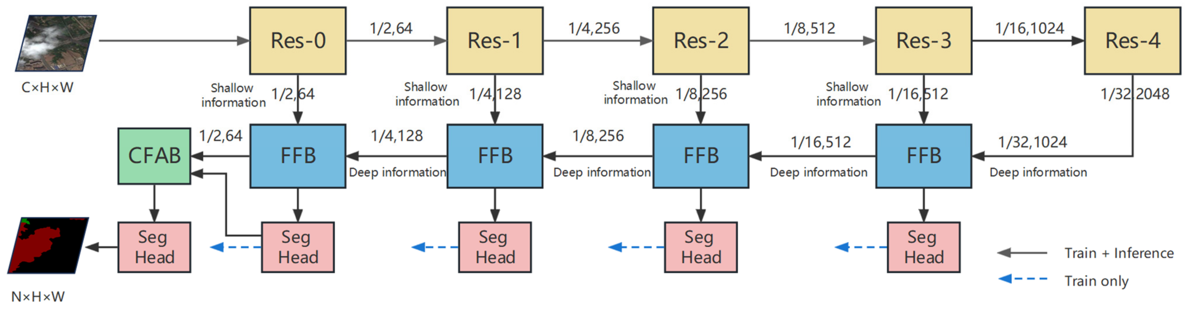
Figure 1.
Framework of our proposed cloud and shadow detection network. Here, C represents the number of channels, N represents the number of classes, and H, W represent the height and width of the input images.
Figure 1.
Framework of our proposed cloud and shadow detection network. Here, C represents the number of channels, N represents the number of classes, and H, W represent the height and width of the input images.
Figure 2.
Feature fusion block. Here, FCB represents the fusion convolution block, CAB represents the channel attention block, and SPA represents the spatial attention block.
Figure 2.
Feature fusion block. Here, FCB represents the fusion convolution block, CAB represents the channel attention block, and SPA represents the spatial attention block.
Figure 3.
Multi-scale convolution block.
Figure 3.
Multi-scale convolution block.
Figure 4.
Channel attention block. Here, represents average pooling, and represents a point-wise convolution layer.
Figure 4.
Channel attention block. Here, represents average pooling, and represents a point-wise convolution layer.
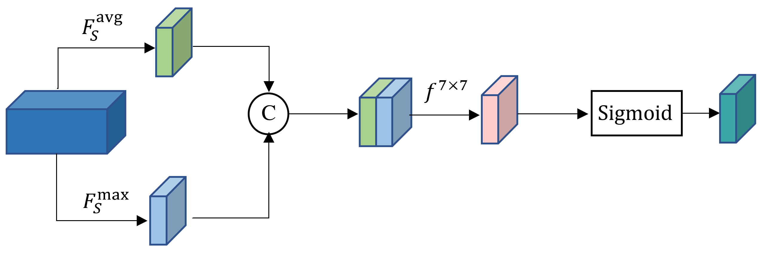
Figure 5.
Spatial attention block. Here, represents average pooling, represents maximum pooling, and represents 7 × 7 convolution.
Figure 5.
Spatial attention block. Here, represents average pooling, represents maximum pooling, and represents 7 × 7 convolution.
Figure 6.
Category feature attention block. Here, represents the number of classes, and represent the channel, height, and width of feature maps.
Figure 6.
Category feature attention block. Here, represents the number of classes, and represent the channel, height, and width of feature maps.
Figure 7.
(a) Test image and its label; (b) heatmaps without CFAB; and (c) heatmaps with CFAB. In (b,c), the top row shows the heatmaps focusing on clouds, while the bottom row shows the heatmaps focusing on cloud shadows. The white and red rectangles highlight the regions where CFAB has made a considerable impact on the model’s performance.
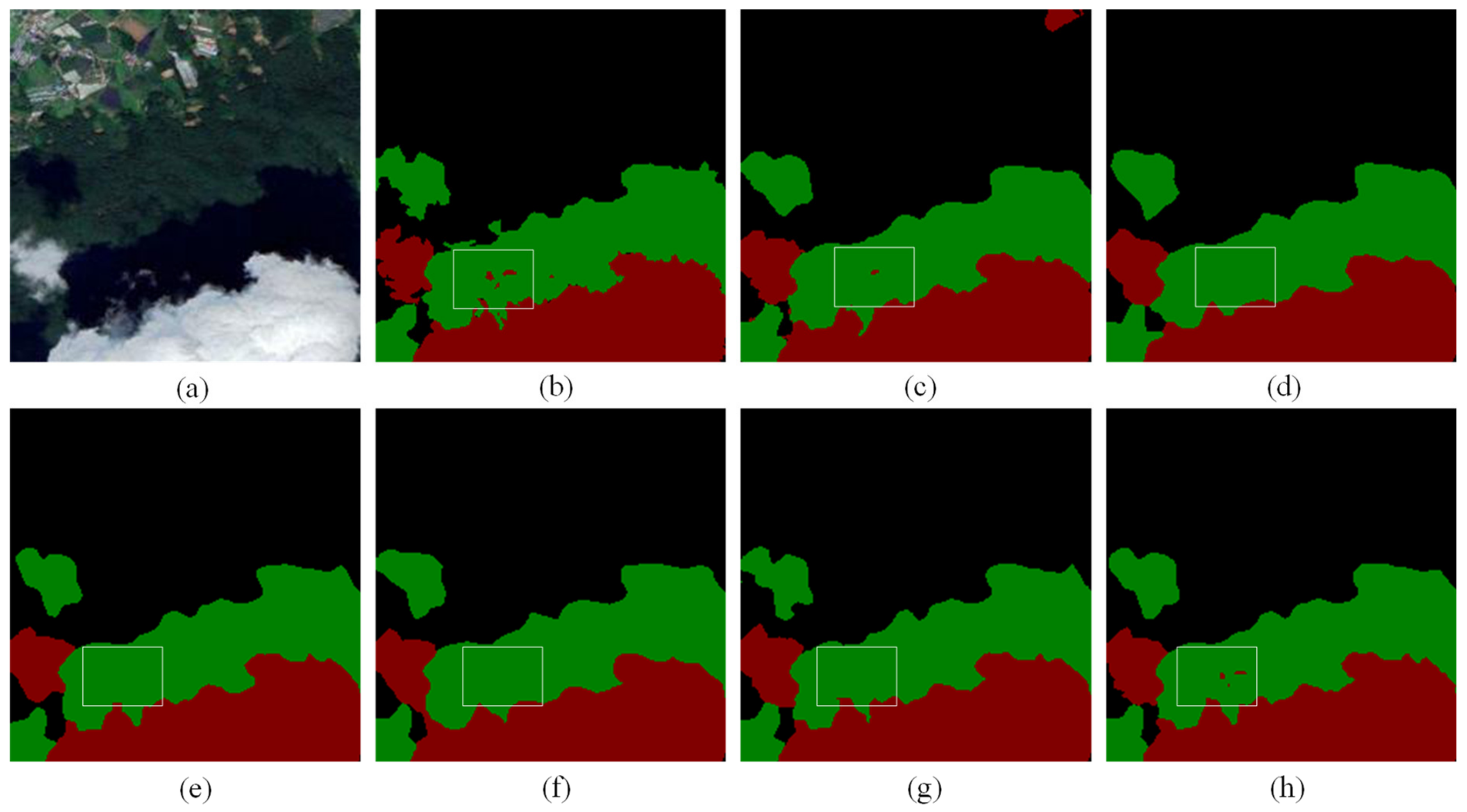
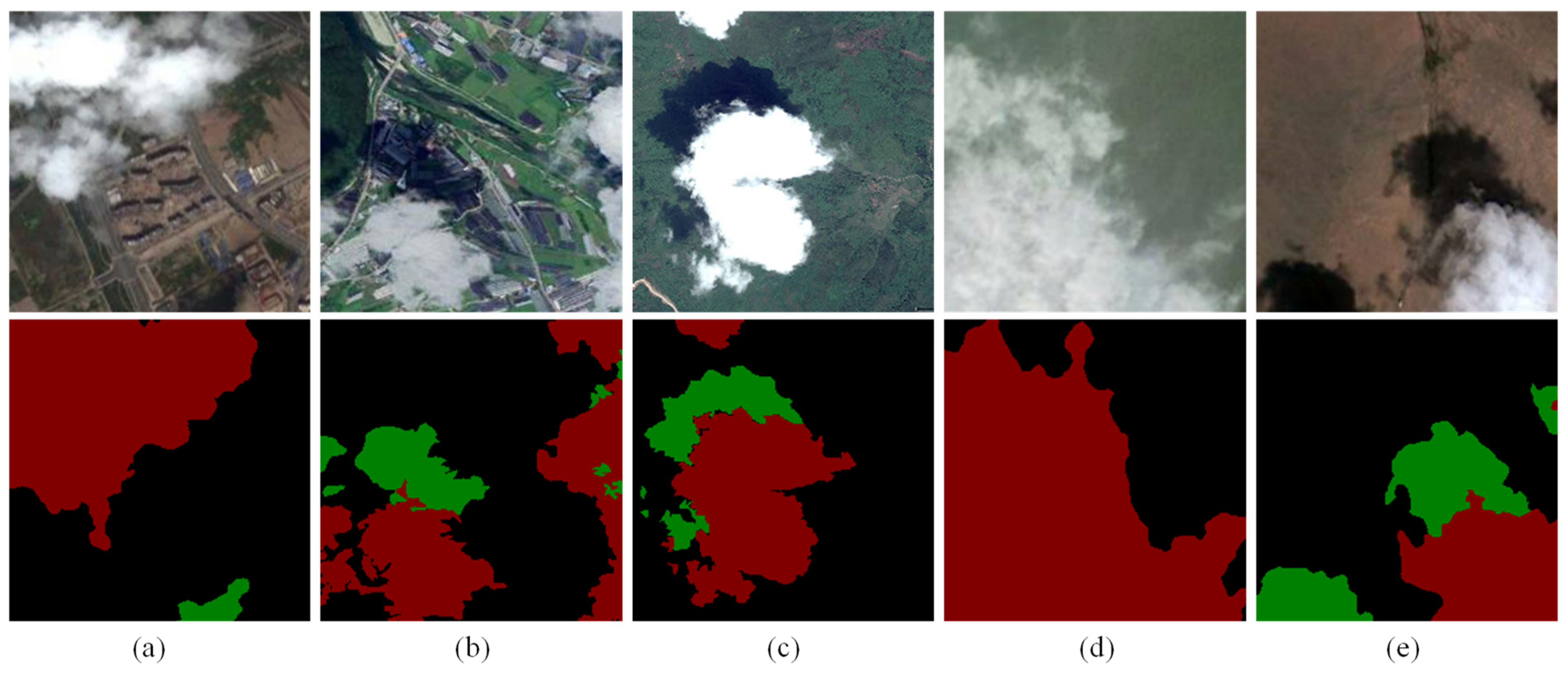
Figure 8.
Some cloud images and their labels against different backgrounds. Clouds, cloud shadows, and backgrounds are marked red, green, and black, respectively. (a) urban areas; (b) farmland areas; (c) plant areas; (d) water areas; and (e) wasteland areas.
Figure 8.
Some cloud images and their labels against different backgrounds. Clouds, cloud shadows, and backgrounds are marked red, green, and black, respectively. (a) urban areas; (b) farmland areas; (c) plant areas; (d) water areas; and (e) wasteland areas.
Figure 9.
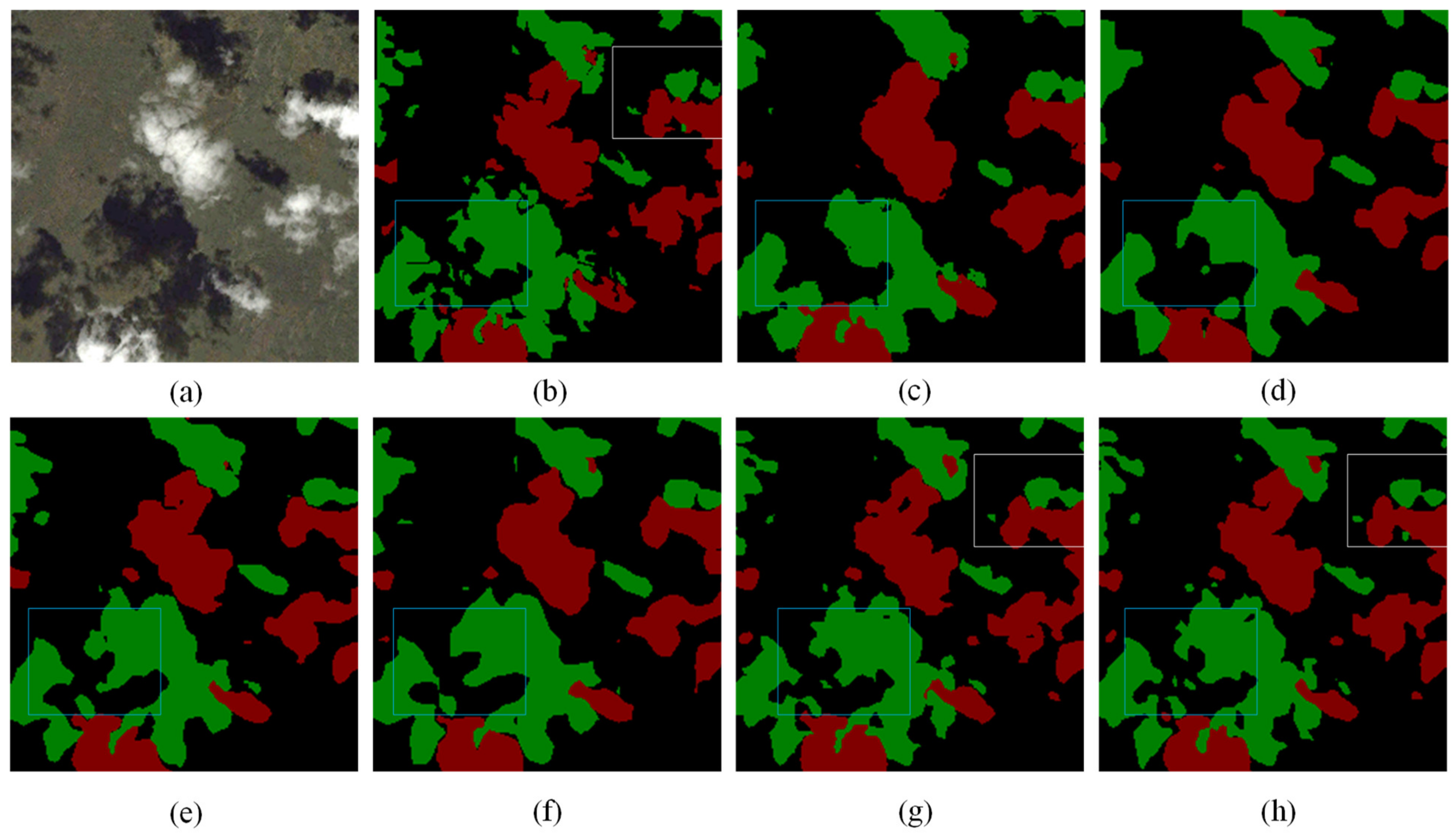
The predicted images of different segmentation models under the plant or farmland area. Clouds, cloud shadows, and backgrounds are marked red, green, and black, respectively. The white rectangles highlight the areas where our model has shown significant improvements compared to other models. (a) The original picture, (b) the label, (c) FCN8s, (d) DeepLabv3+, (e) PSPNet, (f) HRNet, (g) OCRNet, and (h) ours.
Figure 9.
The predicted images of different segmentation models under the plant or farmland area. Clouds, cloud shadows, and backgrounds are marked red, green, and black, respectively. The white rectangles highlight the areas where our model has shown significant improvements compared to other models. (a) The original picture, (b) the label, (c) FCN8s, (d) DeepLabv3+, (e) PSPNet, (f) HRNet, (g) OCRNet, and (h) ours.
Figure 10.
The predicted images of different segmentation models under the wasteland area. Clouds, cloud shadows, and backgrounds are marked red, green, and black, respectively. The white and blue rectangles highlight the areas where our model has shown significant improvements compared to other models. (a) The original picture, (b) the label, (c) FCN8s, (d) DeepLabv3+, (e) PSPNet, (f) HRNet, (g) OCRNet, and (h) ours.
Figure 11.
The predicted images of different segmentation models under the water areas. Clouds, cloud shadows, and backgrounds are marked red, green, and black, respectively. The white and blue rectangles highlight the areas where our model has shown significant improvements compared to other models. (a) The original picture, (b) the label, (c) FCN8s, (d) DeepLabv3+, (e) PSPNet, (f) HRNet, (g) OCRNet, and (h) ours.
Figure 12.
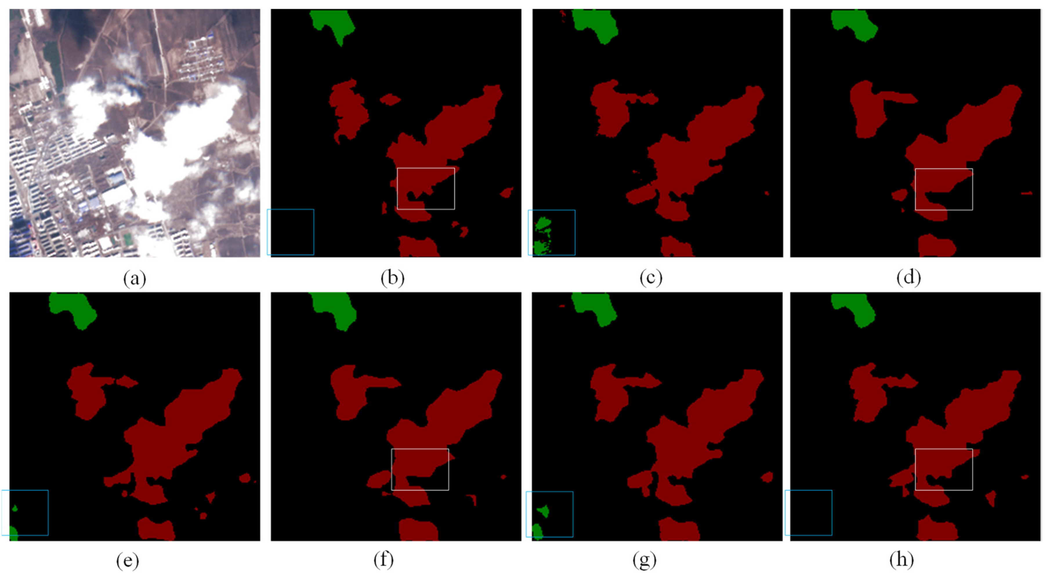
The predicted images of different segmentation models under the urban area. Clouds, cloud shadows, and backgrounds are marked red, green, and black, respectively. The white and blue rectangles highlight the areas where our model has shown significant improvements compared to other models. (a) The original picture, (b) the label, (c) FCN8s, (d) DeepLabv3+, (e) PSPNet, (f) HRNet, (g) OCRNet, and (h) ours.
Figure 12.
The predicted images of different segmentation models under the urban area. Clouds, cloud shadows, and backgrounds are marked red, green, and black, respectively. The white and blue rectangles highlight the areas where our model has shown significant improvements compared to other models. (a) The original picture, (b) the label, (c) FCN8s, (d) DeepLabv3+, (e) PSPNet, (f) HRNet, (g) OCRNet, and (h) ours.
Figure 13.
The predicted images of different segmentation models under the background of vegetation, urban, barren, snow, and water. (a) The original pictures, (b) the labels, (c) DeepLabv3+, (d) OCRNet, (e) PSPNet, and (f) ours.
Figure 13.
The predicted images of different segmentation models under the background of vegetation, urban, barren, snow, and water. (a) The original pictures, (b) the labels, (c) DeepLabv3+, (d) OCRNet, (e) PSPNet, and (f) ours.
Figure 14.
The predicted images of different segmentation algorithms. Clouds, cloud shadows, snow, water, and backgrounds are marked white, black, cyan, blue, and grey, respectively. (a) The original pictures, (b) the labels, (c) DeepLabv3+, (d) HRNet, (e) OCRNet, (f) ours.
Figure 14.
The predicted images of different segmentation algorithms. Clouds, cloud shadows, snow, water, and backgrounds are marked white, black, cyan, blue, and grey, respectively. (a) The original pictures, (b) the labels, (c) DeepLabv3+, (d) HRNet, (e) OCRNet, (f) ours.
Table 1.
Comparison of each ablation model (the best model is in bold).
Table 1.
Comparison of each ablation model (the best model is in bold).
| Models | Parameters (M) | Flops (G) | PA (%) | MIoU (%) |
|---|
| ResNet50 | 27.00 | 4.95 | 96.58 | 92.18 |
| ResNet50 + CAB | 27.53 | 5.17 | 96.93 | 92.79 |
| ResNet50 + FCB + CAB | 43.53 | 7.94 | 97.25 | 93.60 |
| ResNet50 + FCB + CAB + SPA | 43.53 | 7.95 | 97.36 | 93.82 |
| ResNet50 + FCB + CAB + SPA + CFAB | 44.06 | 8.52 | 97.39 | 93.99 |
Table 2.
Comparative cloud and shadow detection results of various algorithms (the best model is in bold).
Table 2.
Comparative cloud and shadow detection results of various algorithms (the best model is in bold).
| Methods | Backbone | PA (%) | mP (%) | mR (%) | F1 (%) | MIoU (%) | FwioU (%) |
|---|
| SegNet [57] | VGG16 | 95.58 | 94.32 | 94.79 | 94.55 | 89.74 | 91.60 |
| U-Net [58] | VGG16 | 96.46 | 95.51 | 95.84 | 95.67 | 91.74 | 93.20 |
| FCN8s [59] | Resnet50 | 96.55 | 95.76 | 95.74 | 95.75 | 91.89 | 93.36 |
| DeepLabv3+ [60] | Resnet50 | 96.85 | 96.09 | 96.18 | 96.14 | 92.59 | 93.91 |
| PSPNet [61] | Resnet50 | 96.96 | 96.25 | 96.30 | 96.28 | 92.85 | 94.12 |
| HRNet [62] | HRNet-W48 | 97.09 | 96.16 | 96.74 | 96.45 | 93.17 | 94.38 |
| OCRNet [54] | HRNet-W48 | 97.30 | 96.63 | 96.80 | 96.71 | 93.66 | 94.76 |
| Ours | Resnet50 | 97.44 | 96.95 | 96.84 | 96.89 | 93.99 | 95.02 |
| Ours | Res2net50 | 97.48 | 97.03 | 96.88 | 96.95 | 94.10 | 95.10 |
Table 3.
The MIoU of our model under different backgrounds (the best model is in bold).
Table 3.
The MIoU of our model under different backgrounds (the best model is in bold).
| Methods | Urban (%) | Farmland (%) | Plant (%) | Water (%) | Wasteland (%) |
|---|
| SegNet | 85.12 | 81.76 | 83.96 | 84.50 | 87.60 |
| U-Net | 85.84 | 82.66 | 84.75 | 85.21 | 88.73 |
| FCN8s | 87.07 | 83.92 | 87.40 | 86.53 | 90.56 |
| DeepLabv3+ | 88.01 | 85.27 | 87.88 | 87.21 | 91.07 |
| PSPNet | 87.60 | 85.28 | 88.13 | 87.29 | 91.30 |
| HRNet | 88.61 | 85.11 | 89.64 | 88.12 | 92.25 |
| OCRNet | 89.22 | 85.40 | 90.05 | 88.30 | 93.77 |
| Ours | 90.38 | 85.98 | 90.74 | 88.94 | 93.90 |
Table 4.
Comparative results of various algorithms on HRC_WHU (the best results are in bold).
Table 4.
Comparative results of various algorithms on HRC_WHU (the best results are in bold).
| Methods | PA (%)
| mP (%) | mR (%) | F1 (%) | MIoU (%)
| FwioU (%) |
|---|
| SegNet | 94.73 | 94.63 | 94.54 | 94.58 | 89.74 | 89.99 |
| UNet | 95.94 | 95.86 | 95.81 | 95.84 | 92.01 | 92.20 |
| HRNet | 95.97 | 95.87 | 95.86 | 95.87 | 92.07 | 92.27 |
| FCN8s | 96.87 | 96.75 | 96.84 | 96.80 | 93.80 | 93.94 |
| DeepLabv3+ | 97.04 | 96.91 | 97.02 | 96.97 | 94.11 | 94.26 |
| OCRNet | 97.24 | 97.14 | 97.19 | 97.16 | 94.49 | 94.63 |
| PSPNet | 97.25 | 97.16 | 97.21 | 97.18 | 94.53 | 94.65 |
| Ours | 97.63 | 97.55 | 97.59 | 97.57 | 95.26 | 95.37 |
Table 5.
Comparative results of different algorithms on SPARCS (the best results are in bold).
Table 5.
Comparative results of different algorithms on SPARCS (the best results are in bold).
| Methods | PA (%) | mP (%) | mR (%) | F1 (%) | MIoU (%) | FwioU (%) |
|---|
| SegNet | 92.19 | 89.46 | 87.64 | 88.48 | 80.07 | 85.80 |
| PSPNet | 95.56 | 94.02 | 92.81 | 93.39 | 87.84 | 91.61 |
| UNet | 95.48 | 93.92 | 92.92 | 93.40 | 87.91 | 91.47 |
| FCN8s | 95.60 | 94.27 | 92.68 | 93.44 | 87.94 | 91.69 |
| DeepLabv3+ | 96.43 | 95.21 | 94.16 | 94.67 | 90.05 | 93.18 |
| HRNet | 96.60 | 95.15 | 94.90 | 95.03 | 90.67 | 93.51 |
| OCRNet | 96.79 | 95.66 | 94.76 | 95.20 | 90.97 | 93.85 |
| Ours | 96.90 | 95.76 | 95.03 | 95.39 | 91.31 | 94.05 |
Table 6.
Comparative results (IoU) of each class obtained by different algorithms on SPARCS (the best model is in bold).
Table 6.
Comparative results (IoU) of each class obtained by different algorithms on SPARCS (the best model is in bold).
| Methods | Clouds (%) | Cloud Shadows (%) | Snow (%) | Water (%) | Backgrounds (%) | Average (%) |
|---|
| SegNet | 81.71 | 59.67 | 89.28 | 78.92 | 90.75 | 80.07 |
| PSPNet | 89.42 | 75.77 | 93.33 | 85.98 | 94.72 | 87.84 |
| UNet | 88.57 | 74.22 | 93.48 | 88.61 | 94.68 | 87.91 |
| FCN8s | 89.59 | 75.97 | 93.41 | 85.95 | 94.75 | 87.94 |
| DeepLabv3+ | 91.45 | 80.31 | 94.50 | 88.27 | 95.72 | 90.05 |
| HRNet | 91.57 | 81.24 | 94.87 | 89.73 | 95.93 | 90.67 |
| OCRNet | 92.39 | 82.46 | 95.05 | 88.78 | 96.15 | 90.97 |
| Ours | 92.41 | 82.63 | 95.26 | 89.90 | 96.32 | 91.31 |


