Abstract
Animal movements are realizations of complex spatiotemporal processes. Central to these processes are the varied environmental contexts in which animals move, which fundamentally impact the movement trajectories of individuals at fine spatial and temporal scales. An emerging perspective in time geography is the direct examination of the influence that varying contexts may have on observed movements. An approach that considers environmental context can yield actionable information for wildlife management, planning, and conservation; for instance, identifying areas of probable occupancy by an animal may improve the efficiency of fieldwork. This research develops the first known practical application of a new cost-distance-based, probabilistic voxel space–time prism (CDBPSTP) in efforts to more realistically characterize the unobserved habitat occupancies of animals occurring between known positions provided by location-aware technologies. The CDBPSTP method is applied to trajectory data collected for a group of red deer (Cervus elaphus) tracked near Banff National Park, Alberta, Canada. As a demonstration of the added value from examining how context influences movement, CDBPSTP habitat occupancy results are compared to the earlier PSTP method in context with empirical and theoretical understandings of red deer habitat preference and space-use behaviors. This comparison reveals that with CDBPSTP, variation present in the mover’s environment is explicitly considered as an influence on the mover’s probable path and occupancies between observations of its location. With the increasing availability of high-resolution geolocational and associated environmental data, this study highlights the potential for CDBPSTP to be leveraged as a broadly applicable tool in animal movement analysis.
1. Introduction
The degree of realism by which we may characterize animal space use is foundationally important to the work of conservationists, biologists, and spatial ecologists interested in understanding patterns and causality in animal movement [1,2,3]. Early work delineated the space of an animal’s daily activity in a deterministic manner based on known animal locations [4,5,6]. Since then, the general practice of estimating animal habitat utilization distributions from geolocation data has developed significantly [7,8,9]. Growth in the literature includes developments in quantifying the time an animal spends in certain areas and how often it returns, and the introduction of three-dimensional movement in kernel utilization distribution analysis [7,8]. With the relatively recent onset of widely available, performant location-aware technologies, the availability and volume of tracking datasets, that is, ordered sets of instantaneous geolocations also termed trajectories, have objectively exploded [10,11,12,13,14,15,16].
This increased availability of movement trajectory data has spurred a wave of new methodologies aimed at extracting meaning for a range of scientific disciplines including spatial ecology and those adjacent. A great deal of these methods are rooted in the early ideas of Time Geography, a theoretical framework first introduced by Hägerstrand (1970) [17]. From the time-geographic perspective, known parameters about the movement of an actor (position, timing, and velocity) can be used to constrain the possible unobserved set of locations the actor may have occupied between known geolocations [18,19]. As a constraints-based perspective on movement, the theoretical tools of time geography include instantaneous geolocations labeled with a timestamp, called space–time anchors; straight-line distances between anchors, called the space–time path; and the bounding set of locations accessible to the moving actor or object, called the space–time prism [19,20,21]. Fundamental to the time geography framework, these objects are shown in Figure 1, with space–time anchors labeled ti and tj. The classical space–time prism is constructed by evaluating a binary accessibility condition (identifying locations as either accessible or not accessible to the mover) for all locations in the space and time elapsed between ti and tj, as a function of the mover’s maximum estimated velocity and the distance each evaluated location deviates from the space–time path.
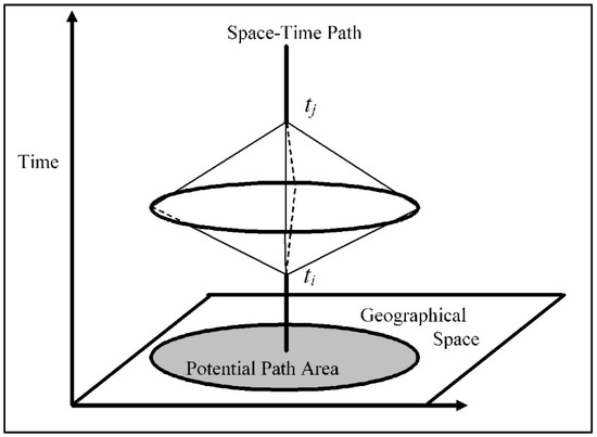
Figure 1.
The Space–time prism [22].
The space–time prism itself has undergone continuing, active development in the literature, with improvements and derivative methods focused on elevating the classical space–time prism from a simple, binary bounding volume for movement possibility toward probabilistic realizations [9,21,23,24]. Further developments include the interactivity among prism volumes [25], prisms that account for uncertainty in anchor locations [26,27], and consideration of kinematics in acceleration and deceleration on the mover [28,29]. Advances in space–time prism construction also introduce the notion of a four-dimensional space–time prism [30] and examine the influence of static spatial context on prism volumes [31,32]. Further still, prism research extends into the examination of the influence that dynamic or temporally modulated factors in the spatial context have on movement [1] and the bounding of prism volumes based on the simulated action of behaviorally informed agent-based models [3]. Advancements in these methods have been demonstrated in application to issues of conservation and wildlife management, enabling better spatiotemporal understandings of animal home range [12], long-distance animal movements [33], and population-level examination of animal habitat use [2]. In particular, research on animal interactions includes animal movement considering the interaction between environmental context and local choice [34], animal-to-animal interactions [25], and animal-to-roadway interactions [1,20,35]. Clearly, incorporating spatiotemporal dynamics into the study of animal movement has proven productive.
Following this pattern of increasing the degree of realism in modeling space–time prisms, the present research seeks to achieve three main goals. First, the authors introduce the method and provide the first known practical application of a new cost-distance-based, probabilistic voxel space–time prism (CDBPSTP). An extension to the probabilistic voxel-based space–time prism (PSTP) [23], CDBPSTP aims for a more realistic characterization of the unobserved habitat occupancies of animals occurring between known locations provided by location-aware technologies. Second, the authors demonstrate the results from CDBPSTP against equivalent results generated by PSTP. Third, the authors discuss the probable impacts and known limitations the method may have following its release as a data analysis tool in forthcoming literature. The results of CDBPSTP are used to explain the method’s advantages and distinctions from similar approaches including PSTP and the field-based method presented in Long (2018) [31]. The present research addresses these objectives by analyzing trajectory data collected for red deer (Cervus elaphus) [36] and modeling the resistance presented to red deer movers in context as a cost surface. The cost surface is derived from a classical habitat selection measure [37,38] and a priori knowledge of red deer habitat preferences. This cost surface is evaluated from variables capturing environmental factors such as terrain and landcover type, along with known animal geolocations as a measure of observed habitat use.
2. Background
2.1. Voxels and Space–Time Prisms
The canonical space–time prism is a well-tested conceptual foundation for a range of studies interested in analyzing movement uncertainty between space–time anchors. In its original formulation, the space–time prism returns only a binary bounding of this uncertainty in terms of space and time [2,19]. For early formulations of the space–time prism, locations between space–time anchors are evaluated to establish whether they were accessible or inaccessible to the mover during the time and space elapsed between the observed space–time anchor locations. Determining the accessibility of each anchor location can be constructed as a piecewise function; the inputs are the mover’s expected maximum velocity, the Euclidean distance from the space–time path to the evaluated location, and time-budgeting parameters derived from the analyzed space–time anchor pair’s spatiotemporal locations (Equation (1)). While formulations for evaluating the space–time prism in continuous space and time exist [21], in practice a discretization of time and space is necessary for simplification and for meeting practical computational concerns [2,23]. One widely employed, atomic-level discretization for this purpose is the voxel, a regularly shaped volume of space (X/Y-axes) and time (Z-axis) for which calculations are evaluated from the perspective of its 3D centroid, and then generalized for the entire volume [22,23,39]. Often, voxel data are modeled in GIScience as regular multidimensional arrays, otherwise known as tensors, stored in a raster data structure or equivalent [22].
where is the Euclidean distance from current voxel centroid location to either space–time anchor location or , is the voxel Z-axis midpoint associated with , and , give the maximum distances the object could have successfully traversed between the anchors, given the time elapsed and remaining between and , respectively, considering the object’s expected maximum speed, .
While early space–time prisms have served in a range of applied studies, the prevailing understanding holds that interior volumes of space–time prisms are not homogeneous, as movement opportunity is not equally distributed over space and time for the mover [1,11,21,23]. As an early improvement on the binary bounding action of the classical space–time prism, Downs et al. (2014) [23] introduced the voxel-based probabilistic space–time prism, where a mover’s chance of having occupied any given voxel location over the time and space elapsed between space–time anchors is assigned as a function of that voxel’s deviation from the space–time path (Equation (2)). This relationship of distance–decay in the probability that a mover will deviate from the shortest path between anchors is reminiscent of theoretical findings on the principle of least effort, applicable in both animal and human mover contexts [40]. Applying the PSTP method, the action of Equation (1) first isolates the set of accessible voxels. Next, Equation (2) assigns occupancy probabilities for voxels, leveraging an inverse-distance weighting function for all voxels present in a particular space–time disk, which is the set of accessible voxels sharing a common z-axis midpoint location, or representing the same unit of duration. Voxel duration (alternatively, voxel Z-axis height) is a user-specified parameter in PSTP; the resulting prism volume will include the number of space–time disks necessary to cover the time elapsed between the space–time anchors analyzed. The sum of probabilities in any given PSTP space–time disk will equal 1.0.
where
is the Euclidean distance between the current voxel centroid location and the intersection location of its host space–time disk , and the space–time path.
Probabilities may be aggregated among disks from a given voxel space–time prism or among disks representing equivalent durations in time between two or more space–time prisms. Prior studies have applied the probabilistic OR operation, in this context referred to as the Comprehensive Probability Surface (CPS) method, dealing with events assumed to be realized from independent spatial processes [23,35]. When aggregating, CPS demands that input space–time disks have the same temporal resolution. For inputs differing in temporal resolution, aggregation to the lowest common multiple among the inputs is necessary. Equation (3) provides the CPS operation on two space–time disks, A and B.
2.2. A Cost-Distance-Based, Probabilistic Voxel Space–Time Prism
Prior work has yielded probabilistic realizations of prism interior volumes following the theoretical principle of least effort [3,40]. A least effort path may reflect the mover’s behavioral or biological preferences, but actual movement is not likely to be linear and does not traverse a perfectly homogeneous surface in terms of movement resistance or conductivity posed by the environment [3,31]. As an exploration in extending the ideas of PSTP toward more realistic constructions of the interior volume of space–time prisms, we introduce the concept of a Cost-Distance-Based, Probabilistic Voxel Space–time Prism (CDBPSTP), along with the ideas of cost distance in the traversal of the environment and a requisite extension to the Time Geography theory, notably a least-cost space–time path.
First, a least-cost space–time path is determined by optimizing for the path of least cumulative cost along a cost surface, which contains values representing the cost of traversing or the willingness of the mover to traverse various environments [41]. For relevant calculations in constructing PSTPs that involve deviation from the space–time path, construction of the CDBPSTP performs these measures in terms of deviation from a least-cost space–time path (Equation (4)). Further, the step bounding accessible voxels in a CDBPSTP also relies on measures based on cost distances (Equation (5)). Together, these extensions yield a prism volume informed in both shape and interior structure by the dynamics of cost distance.
A Cost Surface in this context is a type of map capturing a realistic measure of the resistance or conductance the environment poses to movement for a particular type or species of mover. Cost surfaces may be derived by a range of applicable methods; essentially, the cost surface must capture and represent the relative difficulty or assistance any number of environmental characteristics may pose to the mover of interest. For the present research, we employ the first-known application of habitat selection methodology in space–time prism construction by using habitat selection analysis to inform the multivariate cost surface for the red deer (Cervus elaphus). This approach is detailed in the methods.
where is the cost distance from current voxel centroid location to either space–time anchor location or , is the voxel Z-axis midpoint associated with , and , give the maximum distances the object could have successfully traversed between the anchors, given the time elapsed and remaining between and , respectively, considering the object’s expected maximum speed, .
where is the cost distance of traversal between the current voxel centroid location and the intersection location of its host space–time disk , and the least cost space–time path.
2.3. The Ya Ha Tinda Red Deer Herd
Red deer (Cervus elaphus) are foraging ungulates exhibiting residential and migratory populations in the wild [42]. The red deer (alternatively known by the common name “elk”) population examined for the present study has been researched extensively in the literature [42,43,44]. While red deer have been studied in multiple montane ecosystems [45,46,47,48,49], this research focuses on the herd located in and around Banff National Park (BNP), Alberta, Canada, found along the eastern faces of the front and main ranges of the Canadian Rocky Mountains [42,43]. The Ya Ha Tinda (YHT) herd can be found in the YHT Ranch area located east of BNP, where the residential portion of the herd remains year-round [42,43]. Migration timings for migratory deer were calculated from 1977 to 1980 and from 2002 to 2004 by calculating the midpoint date between two consecutive location points that were each located in a different migratory range [43]. During the spring migration (May or June), migratory individuals move west from the YHT Ranch into BNP and spend the summer season there, before moving back to the YHT grasslands during the autumn migration (late September to November), where they remain through the winter [43]. Compared to the earlier years of the study, roughly 25% of the proportion of the herd that historically migrated in the 1970s continued to do so in 2002 and 2003 [43]. The number of individuals remaining on the YHT range through the summer increased over 10 times from 1977 to 2002–2004, an unexpectedly large increase even when factoring in the simultaneous population growth [43].
3. Methods
3.1. Red Deer Trajectories and Study Area Context
Collar-based tracking data for red deer used in this research were acquired and later released in the public domain by Hebblewhite, Merrill, and McDermid (2008) [42]. This large set of trajectory data generated by their work was obtained through Movebank.org, an online platform cataloging animal tracking data [36]. Hebblewhite et al. (2008) collected these trajectories using GPS and VHF telemetry from 2002 to 2004 in support of research examining the relationship between foraging preferences, environmental factors, and migratory behaviors among red deer in the Canadian Rocky Mountains. The study involved 119 deer, all of whom were female, with 59% of the study group being migratory [42]. The deer were located from the ground or via telemetry aircraft and corresponding GPS data averaged 144 locations per elk (VHF averaged 2.6 locations per elk) every 16-day interval [42].
Defining the bounds of the study area for this research confines interest to areas where the collection interval for data is most consistent, resulting in filtering data to winter-only movement patterns centered on the extent of the YHT Ranch (Figure 2). Study area delineation represents an important methodological step in the approach employed for this research, as the extent of the environmental context underlying selected trajectories establishes the distribution of environmental habitat types available to studied deer.
For cost surface construction, simultaneous analysis of both migratory and residential segments of the tracked population would unfairly represent the distribution of environmental conditions and habitat. Migratory deer typically spend a large amount of time (up to approximately 7 months) within the winter range and shorter time intervals (approximately 2 to 6 days) traversing longer distances during migration periods, and they will have access to different habitat types than residential deer. Even for the migratory deer, habitat types traversed during migration would not be accessible from the winter range. Therefore, the present research has filtered the available trajectories for only those that occur primarily at YHT Ranch. Six deer were shown to be logged relatively consistently for this winter-only period from November to May from 2002 to 2004 with an extent of traversal largely intersecting the YHT Ranch boundary. The deer in this subset represent members of the migratory population performing their routine winter visitation of the YHT Ranch area [42]. Here, limitations related to the degree to which the deer’s usage and availability of environmental characteristics are represented are relaxed by selecting migratory deer found in a common environmental context (the YHT Ranch area) and timeframe (the winter season, during which movements are observed to be more localized compared to longer-distance migratory movement). Descriptive statistics for the six deer trajectories selected and associated winter timeframes are shown in Table 1.

Table 1.
Summary of movement trajectory data for six deer. Two date ranges are necessary due to the split in winter months from the beginning to the end of the year.
Practical study area delineation follows from the selection of trajectories with the application of the Characteristic Hull Polygon (CHP) approach [50] to the complete set of selected geolocations. The CHP represents a deterministic home range delineation method shown to reduce or avoid areal overestimation issues inherent to the often employed minimum convex polygon (MCP) [51] and kernel-density-based methods. Once the CHP boundary was obtained for the trajectories of interest, a buffer having a width of 3178.046473 m was added to accommodate unobserved deer movements beyond the tracked points. First, we identified the mean time elapsed between any two consecutive points across the study dataset. Then, the buffer was set to the longest distance recorded between two consecutive points, where the time elapsed between those points did not exceed the mean time elapsed for the study dataset. Selecting the longest distance between two points based on the mean time elapsed reduces variation caused by varying timespans between location fixes. The buffered CHP boundary represents the final footprint enclosing the available environmental context used for this study (Figure 2).

Figure 2.
Study area with input geolocation data and inputs to the cost surface, with data sources cited in the caption: (A) Bounds of the study area are shown by a blue outline polygon with red deer geolocations in the study dataset represented by points, accompanied by an inset map of western Canada with the study region marked with a red box [36]; (B) The cost surface developed for the study area; (C) Slope in degrees within the study area [52]; (D) Elevation in feet within the study area [52]; (E) Landcover within the study area [53]; and (F) Roads within the study area overlaid on landcover at semi-transparency [54].

3.2. Cost Surface Development Process
Having obtained a boundary that is thought to be reasonably inclusive of unobserved movements, we proceed to evaluate the relative abundances of particular types or factors of the environmental context that underlie deer locations as a proxy for animals’ habitat selections. While environmental context may refer to numerous factors such as predators, competitors, or disease, this study focuses on landcover, elevation, slope, and roadways as representations of the environment in the study area. The ultimate result of this examination is a cost surface reflecting a single variable that represents the degree to which environmental factors are selected or avoided by the YHT population of deer.
Raster datasets depicting landcover type [53,55] and elevation and slope [52] for the study area were collected and clipped to the study area extent as indicators for environmental characteristics (Figure 2, contains information licensed under the Open Government Licence–Canada). The datasets for elevation and slope were classified into eight equal interval ranges. A relatively simple measure of habitat preference in terms of use versus availability, Manly’s selection ratio was applied to obtain a measure of habitat selection or avoidance, given the GPS relocations among the six deer selected as an indication of used habitat types and the proportions of environmental characteristics available within the study area [38] at a p value of 0.05. Operationalized as the function wi in the adehabitatHS R package [37,38], the wi function for Type I design analysis is capable of assessing both habitat availability and usage for a population [56].
Manly’s selection ratio returns higher values for positively selected habitats and lower values for avoided habitat types. Due to this convention, results cannot be directly used to construct a cost raster, which represents increasing cost with increasing magnitude. To translate the resulting Manly selectivity measures to a more conventional resistance surface, rasters for slope, landcover, and elevation were reclassified to their constituent values’ respective Manly selectivity measures, rounded to the nearest integer. In situations where the Manly selectivity measure was near one, corresponding to either very weak selectivity or very weak avoidance, values defaulted to 1.0 to avoid divide-by-zero errors in later analysis. Following the methodology presented in Shafer et al. (2012) [57], all three Manly selectivity measure rasters were transformed into binary rasters depicting habitat selection (a value of 0) or avoidance (a value of 1). One additional binary variable capturing the effect of a 250 m buffer around roadways occurring in the study area was prepared separately from a dataset depicting roads [54], with areas inside the 250 m buffer set as areas of avoidance, consistent with observed red deer preferences in regard to roads [47,58]. Finally, all binary use/avoidance rasters were added together plus a value of 1 to prevent values of 0 from influencing later cost distance calculations to yield a single cost surface (Figure 2).
3.3. Applying CDBPSTP and PSTP to Red Deer Trajectories
The CDBPSTP approach as described in this research has been operationalized in an extension to the PySTPrism toolbox, which is unreleased at the time of this writing [22]. This CDBPSTP implementation was used to generate prism results for the present study. PySTPrism provides a set of voxel-based space–time approaches as an ArcGIS Pro toolbox, compatible with the ArcGIS Pro desktop application from Esri Inc. For each voxel-based prism function found in the toolbox, the interface for the function expects users to supply: (1) an input trajectory dataset as point vector data, (2) the desired X/Y spatial resolution for voxels in the map units of the input data’s coordinate system, (3) the desired Z-axis resolution for voxels in seconds, (4) an optional “Expand Edges” multiple that intentionally expands the processing extent ensuring no results are “cut off” from visualization, and (5) a value for the velocity multiplier parameter. Generating CDBPSTP also requires a cost surface as an input. The velocity multiplier is a value used to scale the observed velocity of the mover between two consecutive space–time anchors; this parameter is meant to account for the assumed straight-line movements captured in trajectories. Since straight-line, top-speed movements are rare for terrestrial animals’ routine traversal in a varied environmental context, the velocity multiplier offers a means to adjust the reachable distances expressed as terms in Equations (4) and (5), such that prism results do not simply converge to the least-cost space–time path, resulting in a prism having zero volume [1,2,22,23].
Selection of an appropriate velocity multiplier value is important, as prism bounds and associated assignment of probabilities are all sensitive to the movement capabilities of the object under study. To realistically estimate a velocity multiplier relating to the actual top speed of red deer tracked for this study, the observed maximum velocity of the trajectory was divided by all observed straight-line velocities for each of the six selected deer trajectories, respectively, producing velocity multipliers specific to sequential pairs of space–time anchors. For each deer, the average of all anchor-pair velocity multipliers yielded a single velocity multiplier tailored toward the individual capabilities of each deer trajectory supplied for CDBPSTP analysis.
The six deer trajectories selected for this analysis contain 11,444 geolocations or fixes in total, reflecting an exhaustive traversal of the YHT ranch area. For the demonstrative goals of this research, representative space–time anchor pairs were extracted from this set, where each selected pair captured a particular movement scenario through the varied context of the study area. To make these selections, 18 anchor pairs representing three distance categories, long (approximately 1100–2000 m), medium (300–800 m), and short (less than 200 m) were isolated (Table 2). The selected anchor pairs were assigned a label associating them with high (predominantly values of 4 and 5), medium (predominantly values of 2, 3, and 4), or low resistance (predominantly values of 1 and 2). Resistance here refers to the values of cells in the cost surface that lie between the two anchors.
Table 2.
Selected space–time anchor pairs illustrating various traversal scenarios in the study area.
Once isolated, each of the 18 anchor pairs and the cost surface were supplied as an input to the CDBPSTP function, with parameters including an output cell size of 30 m, an Expand Edges factor of 1.0, and the velocity multiplier corresponding to the pertinent Deer ID in Table 2. The Expand Edges factor was adjusted as needed. Once CDBPSTP space–time disks were generated, the CPS technique was applied to the disks of each anchor pair to generate occupancy probability surfaces for each pair. To facilitate discussion of the occupancy surface results, zonal descriptive statistics were generated from occupancy surfaces, summarizing the incidence and total probability of occupancy over landcover types. This operation demonstrates an overall view of CDBPSTP’s suggestion of red deer habitat occupancy given the inputs.
To provide a comparison between CDBPSTP and PSTP, this study also generated PSTP occupancy probability surfaces for each anchor pair using the same parameters used to generate CDBPSTPs (sans the input of a cost surface). CPS was applied to these PSTP results in an identical manner. The occupancy probability surfaces for the anchor pairs not detailed directly are provided in the Supplementary Materials for this article. For in-depth detail, one anchor pair was chosen to demonstrate the mechanic difference between PSTP and CDBPSTP, and an additional anchor pair was chosen to demonstrate the practical knowledge that can be derived through CDBPSTP, using landcover as an example. First, the anchor pair labeled Code MH_YL5 represents a medium distance and overall high resistance values and shows the quantitative difference in how CDBPSTP navigates a path across the cost surface, compared to PSTP, which does not consider the cost surface at all. Second, the anchor pair labeled Code ML_29 in Table 2, representing a medium distance and overall lower resistance values, quantifies CDBPSTP’s advantage of revealing information about the environmental factors likely to be chosen by the deer in its movement. The methodology is summarized in Figure 3.
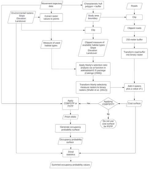
Figure 3.
A flowchart depicting the methods used in this research [37,57].
4. Results
Results pertinent to the expressed targets of this study include the results of Manly’s selection ratio, which represents the analysis product on which the cost surface is based, along with mapping and summary statistics for occupancies returned by CDBPSTP and PSTP prism approaches.
4.1. Results of the wi Function
Pseudo-significance for this measure is expressed in terms of a p-value, interpretable as the magnitude of the chance that returned Manly selectivity values are the result of random chance in habitat selections. For this research, selectivity measures were considered significant if p-values were shown below 0.05, translating roughly to a 95% confidence the results are significant. Manly selectivity measures close to zero indicate avoidance beyond what would be expected at random, given the availability of habitat types and animal selection, while values greater than one demonstrate preference with increasing intensity.
For landcover types occupied, particular results of interest include needleleaf forests and grasslands. Needleleaf forests were highly available in the study area but were weakly selected by deer. Conversely, grasslands were much less abundant but were found to be much more strongly selected by individuals. Considered from the perspective of available animal relocations, roughly 75% of the deer’s locations occurred on grassland, which made up just under 20% of the available study area’s landcover distribution. The Manly selectivity measure represents this interaction as an easily interpreted single-value statistic, found to be significant (by randomization). Urban and built-up and shrubland were also found to show strong selection. Manly selectivity results for landcover classes are shown in Table 3.
Table 3.
Results of the wi function for red deer usage of various landcover classes.
In Table 3, we note an outlying although significant propensity for deer to utilize urban and built-up areas. While it may seem counterintuitive for a soft barrier to result in stronger selection, this is consistent with known red deer behaviors where roadways present a “soft barrier” to traversal [1,35,45,49,59]. Although roads are a soft barrier, the red deer in the study area do traverse the road that runs through the central portion of the YHT Ranch (Figure 2). The behavioral mechanisms underlying this selection may be complex, but considered at a basic level, deer hesitancy to cross a road until traffic has cleared could increase time spent in the vicinity of the road. That additional time could amount to one factor increasing their use of urban and built-up areas. Another possible factor is that the concentration of urban and built-up areas aligns with the road, which runs primarily through grassland. The deer’s strong selection for grassland may cause an increase in time spent in and around the road due to the close vicinity, as the deer moves throughout the preferred grassland.
Manly selectivity measures applied to slopes indicate a general avoidance of areas with slopes exceeding seven degrees in the study area, for the individuals observed (Table 4). It is unknown whether this result is influenced by any particular characteristics common to the tracked individuals or their context; for example, all deer were female, and all geolocations were captured during the winter migration period. Still, this result is consistent with notions of the principle of least effort, where less strenuous routes across the landscape would be preferred [40].
Table 4.
Results of the wi function for red deer usage of various classifications of slope.
Manly selectivity measures for occupied versus available elevation were also calculated. Table 5 summarizes the corresponding Manly selectivity measures for this variable. For elevation, usages are most pronounced between roughly 1500 and 1600 m. This result may be consistent with the occurrence of particular forage or grasses eaten by red deer, especially since higher elevations are related to shorter growing seasons of forage biomass [42]. Higher elevations may be more likely to be associated with other environmental factors such as snow, which requires more energy to navigate for ungulates [60]. In fact, the movement patterns of migratory red deer showed that they moved in lower altitudes as snow cover increased and were more impacted by snow than non-migratory red deer [61]. The selection for relatively lower elevations may also be coincident with the elevation of YHT Ranch and surrounding areas as this location represents high-value habitat overall in the study area. Additionally, the pattern in occupied elevations is generally collinear with the pattern in occupied slope classes. This dynamic could be seen as an illustration of the landscape present in the Banff National Park area itself, an alpine landscape with high local relief in elevation. The complexity inherent to red deer movement behavior along varied terrain and the configuration of their environment may be reflected in this result.
Table 5.
Results of the wi function for red deer usage of various classifications of elevation.
4.2. Results of the CDBPSTP Approach
To demonstrate a comparison in methodology between CDBPSTP and PSTP, representative results for anchor pair MH_YL5 and anchor pair ML_YL29 (see Table 2) were chosen for a detailed presentation. CDBPSTP and PSTP results for all anchor pairs in Table 2 are provided in the Supplementary Materials. The space–time anchor pair MH_YL5 represents movement for Deer YL5′s trajectory and was taken from the animal’s movement in the north-central portion of the study area (51.75291387° N, 115.58246225° W). Figure 4 shows the PSTP occupancy probability surface in panel A, where higher occupancy probabilities are located along a Euclidean space–time path between point 1 and point 2. Figure 4 shows the CDBPSTP occupancy probability surface in panel B, where higher occupancy probabilities lie in a curved shape that places higher likelihoods in areas where the cost surface has lower values. The underlying cost surface is also shown in panel C (Figure 4).
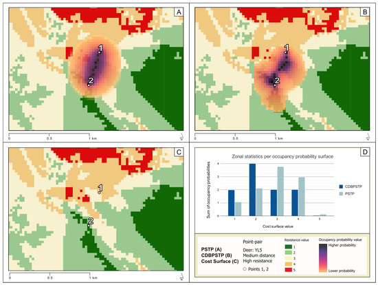
Figure 4.
(A) An occupancy probability surface for anchor pair MH_YL5 overlaid with transparency on the cost surface, generated by the PSTP model, where darker colors signify higher probabilities that the deer was located at that site as it traveled from point 1 to point 2; (B) an occupancy probability surface for anchor pair MH_YL5 overlaid with transparency on the cost surface, generated by the CDBPSTP model based on the cost surface displayed; (C) the cost surface underlying anchor pair MH_YL5; (D) a bar chart depicting zonal statistics where the sum of occupancy probabilities is grouped by cost surface value for both PSTP and CDBPSTP.
The difference in the occupancy probability surfaces generated for anchor pair MH_YL5 is quantified in panel D (Figure 4) and in Table 6. Higher sums of occupancy probability suggest higher chances the deer would have occupied the corresponding cost surface value during its journey between space–time anchors. The sum of CDBPSTP occupancy probabilities grouped by cost surface value shows higher probabilities over lower cost surface values, with the highest summed probability (3.988) over cost surface value 2, followed by 4 (2.006), 3 (1.992), and 1 (1.975) in similar probabilities. In contrast, PSTP shows higher probabilities over higher cost surface values, with the highest summed probability (3.760) over cost surface value 3. While the second-highest summed occupancy probability for PSTP and CDBPSTP are both in cost surface value 4, PSTP (2.948) notes a probability nearly 50% higher than CDBPSTP (2.006). Additionally, the sums of occupancy probabilities for lower cost surface values (1 and 2) under the CDBPSTP method (1.975 and 3.988, respectively) are nearly twice as high as the sums of occupancy probabilities derived through PSTP (1.061 and 2.102, respectively). In other words, across the generated occupancy probability surface, the results of CDBPSTP suggest that the deer had a higher likelihood of being located in sites characterized by lower cost surface values, while PSTP results suggest that the deer was more likely to be located in areas characterized by higher cost surface values.
Table 6.
The sum of occupancy probabilities for the probability surfaces for anchor pair MH_YL5, summed according to the underlying cost surface value.
The second presented space–time anchor pair is from Deer YL29’s trajectory and was taken during the animal’s movement in the central-northeast portion of the study area (51.7467323° N, 115.5366602° W). The traversal shown navigates across an area peripheral to a stand of needleleaf forest, with adjacent shrubland and grassland areas available (panel A, Figure 5). Corresponding resistance values for this environmental context are visualized for the anchor pair in panel B (Figure 5).
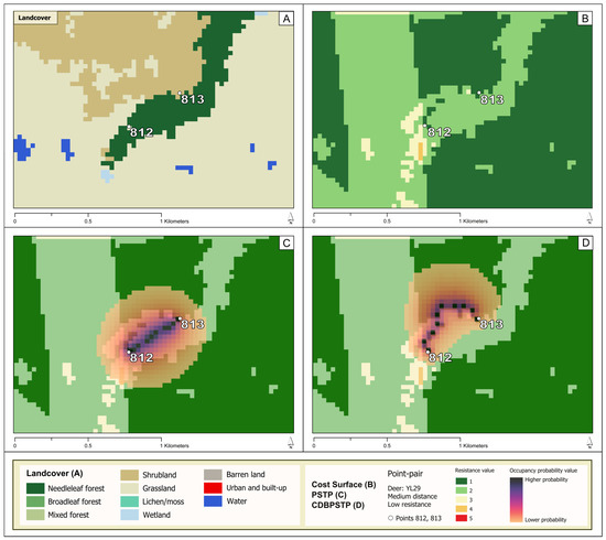
Figure 5.
(A) The landcover underlying anchor pair ML_YL29; (B) the cost surface underlying anchor pair ML_YL29; (C) an occupancy probability surface for anchor pair ML_YL29 overlaid with transparency on the cost surface, generated by the PSTP model, where darker colors signify higher probabilities that the deer was located at that site as it traveled from point 812 to point 813; (D) an occupancy probability surface for anchor pair ML_YL29 overlaid with transparency on the cost surface, generated by the CDBPSTP model based on the cost surface displayed.
Results of the CDBPSTP generated for this anchor pair in context show that according to the animal’s path of traversal reconstructed by CDBPSTP, available shrubland and grassland areas were preferred to passage through needleleaf forest (Figure 5). The animal’s path as suggested by CDBPSTP in Figure 5 denotes an avoidance of areas consistent with a priori knowledge about red deer habitat preferences, ranked using a Manly selectivity approach encoded as cost surface values. A PSTP was also constructed for the anchor pair taken from YL29’s trajectory (Figure 5). Observing the visual comparison between the CDBPSTP and the PSTP (Figure 5) results, the influence of reasonably modeled context on the path of a mover can be significant. The modeled path for CDBPSTP curves noticeably to the north, with higher occupancy probabilities located over lower resistance values in the cost surface.
The dynamic of the influence that the environmental context exerts can be quantified in terms of the summarized occupancy probabilities from each of the CDBPSTP and PSTP results (Table 7). For the CDBPSTP results, the highest probability is associated with shrubland (6.688), followed by grassland (2.243), and needleleaf forest (1.050). In contrast, the PSTP results suggest that needleleaf forest carries the highest probability of occupancy (7.971), followed by shrubland (1.336), and lastly by grassland (0.661). In other words, the probabilistic movements modeled by CDBPSTP suggest that the deer was likely to occupy sites characterized by shrubland, while the results of PSTP suggest a higher likelihood that the deer would occupy needleleaf forest. The two results are in sharp contrast, especially when considering the red deer’s strong selectivity for shrubland and weak selectivity for needleleaf forest (Table 3).
Table 7.
The sum of occupancy probabilities for the probability surfaces for anchor pair ML_YL29, summed according to the underlying landcover type.
5. Discussion
The CDBPSTP approach demonstrated in this study offers an alternative construction of the space–time prism, where the resistances presented by the mover’s environment are explicitly considered as an influence on the probable path and occupancies the mover may have shown between observations of its location. CDBPSTP advances time geographic research on space–time prisms by providing a pathway toward a reasonable incorporation of context in probabilistic space–time prism modeling. This contribution represents an approach applicable toward a better understanding of animal movement and space use, of interest to conservationists, biologists, and planners. CDBPSTP is methodologically separated from its predecessor PSTP by its explicit incorporation of context as a behaviorally informed cost surface.
5.1. Methodological Distinctions of CDBPSTP
The difference between CDBPSTP’s consideration of a cost surface and PSTP’s lack of consideration thereof is shown in Figure 4, where the results of both methods for anchor pair MH_YL5 returned very different occupancy probability surfaces. The PSTP occupancy probability surface shows that a straight-line path from point 1 to point 2 results in higher occupancy probabilities for locations of higher cost surface value (Figure 4). The visualization of PSTP demonstrates its reliance on a Euclidean realization of the space–time path, with assigned occupancy probabilities having magnitudes that are a function of distance–decay from that space–time path. With no consideration of environmental context, the Euclidean-based space–time path is treated as the best-available path when reconstructing a mover’s path between two instantaneous location captures. In contrast, CDBPSTP’s occupancy probability surface exhibits a visible deviation from a Euclidean space–time path as it bends east, away from the cluster of cells on the cost surface that have a resistance value of five. The location of the darker, higher probability areas on the map and the higher sums of occupancy probability in zones of lower cost surface values demonstrate how CDBPSTP incorporates the input environmental context.
Having shown the mechanical differences between PSTP and CDBPSTP, the practical knowledge that can be derived through CDBPSTP is demonstrated in Figure 5, where both methods were applied to anchor pair ML_YL29. The occupancy probabilities for PSTP suggest that deer were more likely to occupy areas of needleleaf forest, while CDBPSTP’s occupancy probabilities suggested a higher likelihood of the deer occupying shrubland (Table 7). Considered in concert with the knowledge that red deer in the YHT Ranch area appear to select for shrubland and grassland over needleleaf forest (Table 3), the value of CDBPSTP as an alternative to PSTP is demonstrated. Visually, the shape of high probability occupancy areas seen in Figure 5 is consistent with CDBPSTP’s methodological notion of a least-cost space–time path, itself is an optimal path of traversal that minimizes travel cost as a function of environmental context. This is an alternative mechanism to the straight-line, Euclidean space–time paths considered in PSTP. Additionally, the distribution of occupancy probabilities that diverge from the least-cost space–time path appears imprinted with the underlying variation in the cost surface. That distribution is a visual indication of the consideration of cost distance when CDBPSTP assigns occupancy probabilities. CDBPSTP is thus shown to capture the influence of a varied environmental context on movement, provided the characterization of this environmental context is rational and fair to the characteristics and observed behaviors of the mover.
CDBPSTP is methodologically separated from similar time-geographic methodologies for estimating animal movement in several ways. Brownian bridge movement models (BBMM) are frequently used to develop animal movement trajectories, but movement between known locations is based on conditional random walks without considering the environmental context in the movement area [9,62]. While the subsequently developed dynamic Brownian bridge movement model (dBBMM) allows for variation in Brownian motion variance (a measure of the animal’s speed, mobility, and movement scale), environmental habitat context is not an input to the model [9,63]. A context-sensitive correlated random walk approach was introduced in a study that does consider the environmental context to generate trajectories, focusing on how local movement choices, pixel-by-pixel, are affected by the environment [34]. CDBPSTP is distinct in the output of the method, generating space–time disks that can be aggregated into a single occupancy probability surface across the extent of the space–time prism rather than developing the probability of visits to a site by generating multiple possible trajectory paths [34].
CDBPSTP is also distinct from the method employing heterogeneous spatial fields [31] due to CDBPSTP’s focus on leveraging cost distance as a derivative of habitat selectivity, and therefore observed animal behavior. Long’s (2018) study considered the environmental context with time-geographic movement analysis of animal movement with the field-based time geography method, which analyzes movement based on the agent’s possible interaction with a cost or resistance surface representing conductance and time cost [31]. The field-based time geography method defines costs in units of time, not distance, and assumes that the agent will move along the shortest-time path between anchor points [31]. In contrast, CDBPSTP’s cost distance relies on the mover’s observed locations to derive a habitat-selection-based cost surface; this may also aid in accounting for habitat selection by animals that change the speed of movement in response to different environments, spending less time in areas of higher predation risk and more time in areas of lower predation risk [64].
5.2. Impacts of Home Range Estimation on CDBPSTP
CDBPSTP results are heavily affected by home range delineation that directly impacts the quantification of resistance that the mover may encounter in the cost surface. Manly’s selection ratio uses the proportion of available habitat types and the proportion of used (or occupied) habitat types to identify which (if any) habitat types are strongly selected [38,65]. For each contextual variable, Manly’s selection ratio compares the count of occupied locations (used habitat types) versus the corresponding count of available locations. An inaccurate estimation of home range would result in inaccurate estimates of available habitat types and habitat selection, ultimately affecting the cost surface.
The first input to Manly’s selection ratio is the set of occupied locations, which consist of the deer GPS location fixes. Under-representation of certain habitats would skew the overall estimate of used habitat. Missing data points in GPS studies may lead to bias that requires additional analysis to correct, particularly in scenarios where mountainous terrain and forest canopy areas impede GPS collar data acquisition, although GPS collars were shown to perform better over time [66].
The second input to Manly’s selection ratio is the set of available habitat types, determined by the home range delineation. In this application, CHP was used instead of MCP, which has been demonstrated to introduce biases resulting in inaccurate estimations of the home range [50,63,67]. Additionally, MCP’s sensitivity to varying properties of the data, such as data outliers, spatial resolution, and sample size, means that it cannot be comparable among different studies [68,69]. Even though the buffered study area for this research does include areas that would have been enclosed by an MCP, the buffer itself is not building on potential overestimations that may have already existed in an MCP. By starting with CHP, the buffer allows for the fact that elk are not necessarily confined to the locations recorded. The buffer simply encloses environmental features that are considered available to the studied individuals during the winter season, as the deer can reasonably be expected to move beyond the recorded data points.
Kernel density estimation (KDE) has also been widely used to calculate home range from spatial point data, and adaptations have improved selection for sensitive parameters such as bandwidth, which is the radius of a circular area placed over each point to calculate density defined by a kernel function [69,70,71]. KDE bandwidth selection significantly influences the resulting home range, but selection methods are often not reported and the method of setting a volume contour (which specifies the bounds of the home range) is similarly impactful yet still requires development [63,69].
The BBMM approach is also commonly used to estimate home range based on an animal’s movement trajectory, rather than treating the geo-points of a trajectory as independent locations [62,63]. BBMMs have been used in the literature to estimate the home range for red deer, but this study chose to use the CHP method rather than using a trajectory-based method to generate a home range estimate that would subsequently affect the results of estimated movements under CDBPSTP [72]. Further research carrying out a full comparison of how trajectory-based home ranges (like BBMM or dBBMM) versus polygon-based home ranges (like CHP) affect CDBPSTP results would significantly contribute to the understanding of home range estimation impacts on CDBPSTP construction.
5.3. Limitations
Limitations associated with the approach in its current demonstration center on sensitivity to home range delineation as discussed, issues of scale and generalization, and future validation. The present study conducted an involved analysis of the habitat selectivity of a particular red deer population in a highly selected study area and used the results to inform the cost surface. This cost surface is tightly coupled to both the study area and population. Applying the resistance valuation scheme generated for this research to similar studies on red deer in different locations could amount to Ecological Fallacy. Conducting a broader selectivity analysis on a wider range of input data that represent a larger population regionally may enable a wider application of a generated cost surface. Creating a regional cost surface would require an area of consistent environmental habitat and a study population that exhibits consistent behaviors. The resistance valuation scheme of the resulting cost surface for a larger region, such as a broader portion of BNP, could be applied to a wider range of data within that region.
A practical aspect affecting applicability is the time needed to generate occupancy probability surfaces. For each CDBPSTP generated for the geolocation anchor pairs in this study (see Table 2), total processing time varied between 10 and 15 min, with the processing time naturally increasing as the distance between anchor pairs and spatial resolution of voxels is increased. Expanding the scale of application, for example, analyzing a large population or long-range movements, requires additional computational time. Automating the functions in the PySTPrism toolbox will reduce the amount of active processing time and enable greater applicability to varied datasets.
With respect to validation, the present study has not sought to establish any measure of internal stability in the results. Ensuring that the CDBPSTP approach behaves predictably (considering relatively consistent inputs) is a step supporting its adoption for future studies. Considering the computational time required, this study’s smaller dataset is suitable to meet the scope of demonstrating this new method; further work can use a larger trajectory dataset to implement validation techniques. There are at least two possible routes for validation. First, a full comparison of CDBPSTP and PSTP can test data with varying temporal intervals, environments, and distances between points to assess whether either method is more suitable for certain types of data. Both methods can be applied to temporally non-contiguous points, such as the first and the fifth points in a trajectory. The movement probabilities in the resulting occupancy probability surfaces may be compared to the trajectory’s intermediate points of known locations (in this example, the second through fourth points). Comparing the results of both methods can determine which, if either, better reconstructed the agent’s movements. Such a comparison would have practical benefits because the PSTP method does not require the construction of a cost surface and is, therefore, more straightforward and faster to implement. If PSTP is shown to suitably reconstruct movement for certain types of trajectories, it may be particularly useful for studies hindered by a lack of environmental data. A formal evaluation of the CDBPSTP method’s performance can also help define the extent of CDBPSTP’s ability in understanding animal movement, highlight key areas of the method that would benefit from further development, and provide a foundation on which to build environment-incorporating time-geographic approaches. Another validation approach in future research could apply the cost surface and CDBPSTP methodology to data collected during other timeframes for the same population and compare the results via some two-dimensional measure in the separation of distributions, perhaps Bhattacharyya distance. In any case, both these “prior” and “future” datasets should be collected under similar conditions.
Further advancement in determining the velocity multiplier parameter represents a growth area not just for CDBPSTP research, but for probabilistic space–time prism applications in general. CDBPSTP is shown to be highly sensitive to the selection and application of the velocity multiplier, as this value corresponds to an estimate of the mover’s top speed, therefore setting the extent and interior structure of the resulting prism volume. For the present study, an averaged maximum observed velocity to individual anchor-pair velocity ratio was calculated for each individual animal. For a mover traversing a real-world context, the actual top speed is both unknown at any given time and may be serially influenced by both the last location traversed and the next location ahead of the mover. This translates to infinitely many possible realizations of top speed between any two space–time anchors in context. Also, the behavioral dynamics governing whether the mover intended to reach a top speed between anchors cannot be known. CDBPSTP, like other space–time prism methods, always sets outer bounds based on a maximum velocity we assume the mover can achieve. It is possible that future research could include video or secondary observation of the mover contemporaneous with the collection of space–time anchors/GPS fixes such that some of this dynamic might be described and incorporated into velocity multiplier calculations.
The results of this study have shown that CDBPSTP explicitly considers variation present in a moving agent’s environment and shows the influence that environmental context may have on the probable movements between known locations. This work also shows CDBPSTP is compatible with habitat selection analysis, and the methodology is applicable to species other than red deer because it bases the estimated probability of movement on the population’s specific observed preferences. As a result, different species’ habitat preferences can be represented and considered in the estimation of movements. A multitude of practical benefits stems from the incorporation of environmental context. A more realistic estimate of animal movements can help narrow down the possible areas where animals are likely to be located, which can decrease the time and resources spent on fieldwork in conservational or related efforts to locate specific animals. Understanding how different species move through different topographies and landcover types can help wildlife management by informing the consequences of changing natural features. For example, if a species shows high occupancy probabilities in forested regions, deforestation may carry a higher likelihood of concentrating the population’s movements in a smaller area, which can affect subsequent habitat usage and movement behaviors. CDBPSTP’s incorporation of environmental context is an important move toward a more informed understanding of animal movements, beneficial both for conservation efforts now and for future responses to changes in the environment.
Supplementary Materials
The following supporting information can be downloaded at https://www.mdpi.com/article/10.3390/ijgi12080339/s1. All anchor pairs listed in Table 2 were evaluated through both PSTP and CDBPSTP and were found to be consistent with the results reported for the two anchor pairs detailed in the article. The Supplementary Materials contain occupancy probability surfaces for all the other anchor pairs that were not included in the main article, showing both CDBPSTP and PSTP results. Each anchor pair’s occupancy probability surfaces are shown side by side, with PSTP results on the left and CDBPSTP results on the right. Direction of movement can be noted through the point labels, where movement is from the lower number to the higher number. Additional details on the deer from which the points were taken can be found in Table 2 by locating the deer ID (top left corner of each panel) and the point labels. The Supplementary Materials also include tables denoting the sum of occupancy probabilities for occupancy probability surfaces for each anchor pair not shown in the main text, summed according to the underlying cost surface value. Figure S1: Occupancy probability surfaces for anchor pairs considered to have a long-distance range between points, overlaid with transparency on the cost surface. Panels on the left were generated by the PSTP model, and panels on the right were generated by the CDBPSTP model. Each panel is labeled by Deer ID and each point is labeled by Point Location ID. Darker colors signify higher probabilities that the deer was located at that site as it traveled between points. Figure S2: Occupancy probability surfaces for anchor pairs considered to have a medium-distance range between points, overlaid with transparency on the cost surface. Panels on the left were generated by the PSTP model, and panels on the right were generated by the CDBPSTP model. Each panel is labeled by Deer ID and each point is labeled by Point Location ID. Darker colors signify higher probabilities that the deer was located at that site as it traveled between points. Figure S3: Occupancy probability surfaces for anchor pairs considered to have a short-distance range between points, overlaid with transparency on the cost surface. Panels on the left were generated by the PSTP model, and panels on the right were generated by the CDBPSTP model. Each panel is labeled by Deer ID and each point is labeled by Point Location ID. Darker colors signify higher probabilities that the deer was located at that site as it traveled between points. Table S1: The sum of occupancy probabilities for the occupancy probability surfaces for anchor pairs considered to have a long-distance range between points, summed according to the underlying cost surface value. Table S2: The sum of occupancy probabilities for the occupancy probability surfaces for anchor pairs considered to have a medium-distance range between points, summed according to the underlying cost surface value. Table S3: The sum of occupancy probabilities for the occupancy probability surfaces for anchor pairs considered to have a short-distance range between points, summed according to the underlying cost surface value.
Author Contributions
Conceptualization, Rebecca Loraamm and Katherine Ho; methodology, Rebecca Loraamm; software, Rebecca Loraamm; validation, Katherine Ho; formal analysis, Rebecca Loraamm and Katherine Ho; investigation, Katherine Ho; resources, Rebecca Loraamm; data curation, Katherine Ho; writing—original draft preparation, Katherine Ho; writing—review and editing, Rebecca Loraamm and Katherine Ho; visualization, Katherine Ho; supervision, Rebecca Loraamm; project administration, Rebecca Loraamm and Katherine Ho; funding acquisition, not applicable. All authors have read and agreed to the published version of the manuscript.
Funding
This research received no external funding.
Data Availability Statement
The data presented in this study are openly available in Movebank Data Repository at https://doi.org/10.5441/001/1.k8s2g5v7/1.
Conflicts of Interest
The authors declare no conflict of interest.
References
- Loraamm, R.; Anderson, J.; Burch, C. Identifying Road Avoidance Behavior Using Time-Geography for Red Deer in Banff National Park, Alberta, Canada. Trans. GIS 2021, 25, 1331–1346. [Google Scholar] [CrossRef]
- Loraamm, R.W.; Goodenough, K.S.; Burch, C.; Davenport, L.C.; Haugaasen, T. A Time-Geographic Approach to Identifying Daily Habitat Use Patterns for Amazonian Black Skimmers. Appl. Geogr. 2020, 118, 102189. [Google Scholar] [CrossRef]
- Loraamm, R.W. Incorporating Behavior into Animal Movement Modeling: A Constrained Agent-Based Model for Estimating Visit Probabilities in Space-Time Prisms. Int. J. Geogr. Inf. Sci. 2020, 34, 1607–1627. [Google Scholar] [CrossRef]
- Burt, W.H. Territoriality and Home Range Concepts as Applied to Mammals. J. Mammal. 1943, 24, 346–352. [Google Scholar] [CrossRef]
- Worton, B.J. A Review of Models of Home Range for Animal Movement. Ecol. Model. 1987, 38, 277–298. [Google Scholar] [CrossRef]
- Worton, B.J. Using Monte Carlo Simulation to Evaluate Kernel-Based Home Range Estimators. J. Wildl. Manag. 1995, 59, 794–800. [Google Scholar] [CrossRef]
- Benhamou, S.; Riotte-Lambert, L. Beyond the Utilization Distribution: Identifying Home Range Areas That Are Intensively Exploited or Repeatedly Visited. Ecol. Model. 2012, 227, 112–116. [Google Scholar] [CrossRef]
- Khosravifard, S.; Skidmore, A.K.; Naimi, B.; Venus, V.; Muñoz, A.R.; Toxopeus, A.G. Identifying Birds’ Collision Risk with Wind Turbines Using a Multidimensional Utilization Distribution Method. Wildl. Soc. Bull. 2020, 44, 191–199. [Google Scholar] [CrossRef]
- Kranstauber, B.; Kays, R.; LaPoint, S.D.; Wikelski, M.; Safi, K. A Dynamic Brownian Bridge Movement Model to Estimate Utilization Distributions for Heterogeneous Animal Movement. J. Anim. Ecol. 2012, 81, 738–746. [Google Scholar] [CrossRef] [PubMed]
- Cagnacci, F.; Boitani, L.; Powell, R.A.; Boyce, M.S. Animal Ecology Meets GPS-Based Radiotelemetry: A Perfect Storm of Opportunities and Challenges. Philos. Trans. R. Soc. B Biol. Sci. 2010, 365, 2157–2162. [Google Scholar] [CrossRef]
- Dodge, S.; Weibel, R.; Ahearn, S.C.; Buchin, M.; Miller, J.A. Analysis of Movement Data. Int. J. Geogr. Inf. Sci. 2016, 30, 825–834. [Google Scholar] [CrossRef]
- Long, J.; Nelson, T. Home Range and Habitat Analysis Using Dynamic Time Geography. J. Wildl. Manag. 2015, 79, 481–490. [Google Scholar] [CrossRef]
- Farley, S.S.; Dawson, A.; Goring, S.J.; Williams, J.W. Situating Ecology as a Big-Data Science: Current Advances, Challenges, and Solutions. BioScience 2018, 68, 563–576. [Google Scholar] [CrossRef]
- Kays, R.; Davidson, S.C.; Berger, M.; Bohrer, G.; Fiedler, W.; Flack, A.; Hirt, J.; Hahn, C.; Gauggel, D.; Russell, B.; et al. The Movebank System for Studying Global Animal Movement and Demography. Methods Ecol. Evol. 2022, 13, 419–431. [Google Scholar] [CrossRef]
- Qian, C.; Yi, C.; Cheng, C.; Pu, G.; Wei, X.; Zhang, H. GeoSOT-Based Spatiotemporal Index of Massive Trajectory Data. ISPRS Int. J. Geo-Inf. 2019, 8, 284. [Google Scholar] [CrossRef]
- Wang, D.; Miwa, T.; Morikawa, T. Big Trajectory Data Mining: A Survey of Methods, Applications, and Services. Sensors 2020, 20, 4571. [Google Scholar] [CrossRef] [PubMed]
- Hägerstrand, T. What about People in Regional Science? Pap. Reg. Sci. 1970, 24, 7–24. [Google Scholar] [CrossRef]
- Miller, H.J. A Measurement Theory for Time Geography. Geogr. Anal. 2005, 37, 17–45. [Google Scholar] [CrossRef]
- Miller, H.J. Time Geography and Space-Time Prism. In International Encyclopedia of Geography: People, the Earth, Environment and Technology; Richardson, D., Castree, N., Goodchild, M.F., Kobayashi, A., Liu, W., Marston, R.A., Eds.; John Wiley & Sons, Ltd.: Oxford, UK, 2017; pp. 1–19. ISBN 978-0-470-65963-2. [Google Scholar]
- Loraamm, R.W.; Downs, J.A.; Lamb, D. A Time-Geographic Approach to Quantifying Wildlife–Road Interactions. Trans. GIS 2019, 23, 70–86. [Google Scholar] [CrossRef]
- Winter, S.; Yin, Z.-C. The Elements of Probabilistic Time Geography. Geoinformatica 2011, 15, 417–434. [Google Scholar] [CrossRef]
- Loraamm, R.; Downs, J.; Anderson, J.; Lamb, D.S. PySTPrism: Tools for Voxel-Based Space–Time Prisms. SoftwareX 2020, 12, 100499. [Google Scholar] [CrossRef]
- Downs, J.A.; Horner, M.W.; Hyzer, G.; Lamb, D.; Loraamm, R. Voxel-Based Probabilistic Space-Time Prisms for Analysing Animal Movements and Habitat Use. Int. J. Geogr. Inf. Sci. 2014, 28, 875–890. [Google Scholar] [CrossRef]
- Song, Y.; Miller, H.J. Simulating Visit Probability Distributions within Planar Space-Time Prisms. Int. J. Geogr. Inf. Sci. 2014, 28, 104–125. [Google Scholar] [CrossRef]
- Downs, J.A.; Lamb, D.; Hyzer, G.; Loraamm, R.; Smith, Z.J.; O’Neal, B.M. Quantifying Spatio-Temporal Interactions of Animals Using Probabilistic Space–Time Prisms. Appl. Geogr. 2014, 55, 1–8. [Google Scholar] [CrossRef]
- Kuijpers, B.; Miller, H.J.; Neutens, T.; Othman, W. Anchor Uncertainty and Space-Time Prisms on Road Networks. Int. J. Geogr. Inf. Sci. 2010, 24, 1223–1248. [Google Scholar] [CrossRef]
- Kuijpers, B.; Othman, W. The Geometry of Space-Time Prisms with Uncertain Anchors. Int. J. Geogr. Inf. Sci. 2017, 31, 1722–1748. [Google Scholar] [CrossRef]
- Long, J.A. Kinematic Interpolation of Movement Data. Int. J. Geogr. Inf. Sci. 2016, 30, 854–868. [Google Scholar] [CrossRef]
- Long, J.A.; Nelson, T.A.; Nathoo, F.S. Toward a Kinetic-Based Probabilistic Time Geography. Int. J. Geogr. Inf. Sci. 2014, 28, 855–874. [Google Scholar] [CrossRef]
- Demšar, U.; Long, J.A. Potential Path Volume (PPV): A Geometric Estimator for Space Use in 3D. Mov. Ecol. 2019, 7, 14. [Google Scholar] [CrossRef]
- Long, J.A. Modeling Movement Probabilities within Heterogeneous Spatial Fields. J. Spat. Inf. Sci. 2018, 16, 85–116. [Google Scholar] [CrossRef]
- Miller, H.J.; Bridwell, S.A. A Field-Based Theory for Time Geography. Ann. Assoc. Am. Geogr. 2009, 99, 49–75. [Google Scholar] [CrossRef]
- Kuijpers, B.; Technitis, G. Space-Time Prisms on a Sphere with Applications to Long-Distance Movement. Int. J. Geogr. Inf. Sci. 2020, 34, 1980–2003. [Google Scholar] [CrossRef]
- Ahearn, S.C.; Dodge, S.; Simcharoen, A.; Xavier, G.; Smith, J.L.D. A Context-Sensitive Correlated Random Walk: A New Simulation Model for Movement. Int. J. Geogr. Inf. Sci. 2017, 31, 867–883. [Google Scholar] [CrossRef]
- Loraamm, R.; Downs, J. A Wildlife Movement Approach to Optimally Locate Wildlife Crossing Structures. Int. J. Geogr. Inf. Sci. 2016, 30, 74–88. [Google Scholar] [CrossRef]
- Hebblewhite, M.; Merrill, E. Data from: A Multi-Scale Test of the Forage Maturation Hypothesis in a Partially Migratory Ungulate Population. Movebank Data Repos. 2008. [Google Scholar] [CrossRef]
- Calenge, C. The Package “Adehabitat” for the R Software: A Tool for the Analysis of Space and Habitat Use by Animals. Ecol. Model. 2006, 197, 516–519. [Google Scholar] [CrossRef]
- Manly, B.F.; McDonald, L.; Thomas, D.L.; McDonald, T.L.; Erickson, W.P. Resource Selection by Animals: Statistical Design and Analysis for Field Studies, 2nd ed.; Springer: Dordrecht, The Netherlands, 2002; ISBN 978-0-306-48151-2. [Google Scholar]
- Huisman, O.; Forer, P. Computational Agents and Urban Life Spaces: A Preliminary Realisation of the Time-Geography of Student Lifestyles. In Proceedings of the Proceedings of the Third International Conference on GeoComputation, Bristol, UK, 17-19 September 1998; p. 18. [Google Scholar]
- Zipf, G.K. Human Behavior and the Principle of Least Effort; Addison-Wesley Press: Boston, MA, USA, 1949. [Google Scholar]
- Zeller, K.A.; McGarigal, K.; Whiteley, A.R. Estimating Landscape Resistance to Movement: A Review. Landsc. Ecol. 2012, 27, 777–797. [Google Scholar] [CrossRef]
- Hebblewhite, M.; Merrill, E.; McDermid, G. A Multi-Scale Test of the Forage Maturation Hypothesis in a Partially Migratory Ungulate Population. Ecol. Monogr. 2008, 78, 141–166. [Google Scholar] [CrossRef]
- Hebblewhite, M.; Merrill, E.H.; Morgantini, L.E.; White, C.A.; Allen, J.R.; Bruns, E.; Thurston, L.; Hurd, T.E. Is the Migratory Behavior of Montane Elk Herds in Peril? The Case of Alberta’s Ya Ha Tinda Elk Herd. Wildl. Soc. Bull. 2006, 34, 1280–1294. [Google Scholar] [CrossRef]
- Sachro, L.L.; Strong, W.L.; Gates, C.C. Prescribed Burning Effects on Summer Elk Forage Availability in the Subalpine Zone, Banff National Park, Canada. J. Environ. Manag. 2005, 77, 183–193. [Google Scholar] [CrossRef] [PubMed]
- Ciuti, S.; Muhly, T.B.; Paton, D.G.; McDevitt, A.D.; Musiani, M.; Boyce, M.S. Human Selection of Elk Behavioural Traits in a Landscape of Fear. Proc. R. Soc. B Biol. Sci. 2012, 279, 4407–4416. [Google Scholar] [CrossRef] [PubMed]
- Hebblewhite, M.; Merrill, E.H. Trade-Offs between Predation Risk and Forage Differ between Migrant Strategies in a Migratory Ungulate. Ecology 2009, 90, 3445–3454. [Google Scholar] [CrossRef] [PubMed]
- Meisingset, E.L.; Loe, L.E.; Brekkum, Ø.; Van Moorter, B.; Mysterud, A. Red Deer Habitat Selection and Movements in Relation to Roads. J. Wildl. Manag. 2013, 77, 181–191. [Google Scholar] [CrossRef]
- Middleton, A.D.; Kauffman, M.J.; McWhirter, D.E.; Cook, J.G.; Cook, R.C.; Nelson, A.A.; Jimenez, M.D.; Klaver, R.W. Animal Migration amid Shifting Patterns of Phenology and Predation: Lessons from a Yellowstone Elk Herd. Ecology 2013, 94, 1245–1256. [Google Scholar] [CrossRef] [PubMed]
- Prokopenko, C.M.; Boyce, M.S.; Avgar, T. Characterizing Wildlife Behavioural Responses to Roads Using Integrated Step Selection Analysis. J. Appl. Ecol. 2017, 54, 470–479. [Google Scholar] [CrossRef]
- Downs, J.A.; Horner, M.W. A Characteristic-Hull Based Method for Home Range Estimation. Trans. GIS 2009, 13, 527–537. [Google Scholar] [CrossRef]
- Mohr, C.O. Table of Equivalent Populations of North American Small Mammals. Am. Midl. Nat. 1947, 37, 223–249. [Google Scholar] [CrossRef]
- Natural Resources Canada Data from: Canadian Digital Elevation Model. Contains Information Licensed under the Open Government Licence—Canada. Available online: https://maps.canada.ca/czs/index-en.html (accessed on 21 August 2020).
- Latifovic, R. 2010 Land Cover of Canada. Contains Information Licensed under the Open Government Licence—Canada. Available online: https://open.canada.ca/data/en/dataset/c688b87f-e85f-4842-b0e1-a8f79ebf1133 (accessed on 20 October 2020).
- Statistics Canada Data from: Statistics Canada. Road Network File—2009—Alberta. Contains Information Licensed under the Open Government Licence—Canada. Available online: https://open.canada.ca/data/en/dataset/8f7d56c5-c7ad-4ca0-8a7f-b1e2d0d46e5b (accessed on 20 October 2020).
- Latifovic, R.; Pouliot, D.; Olthof, I. Circa 2010 Land Cover of Canada: Local Optimization Methodology and Product Development. Remote Sens. 2017, 9, 1098. [Google Scholar] [CrossRef]
- Thomas, D.L.; Taylor, E.J. Study Designs and Tests for Comparing Resource Use and Availability. J. Wildl. Manag. 1990, 54, 322–330. [Google Scholar] [CrossRef]
- Shafer, A.B.A.; Northrup, J.M.; White, K.S.; Boyce, M.S.; Côté, S.D.; Coltman, D.W. Habitat Selection Predicts Genetic Relatedness in an Alpine Ungulate. Ecology 2012, 93, 1317–1329. [Google Scholar] [CrossRef]
- Gagnon, J.W.; Theimer, T.C.; Boe, S.; Dodd, N.L.; Schweinsburg, R.E. Traffic Volume Alters Elk Distribution and Highway Crossings in Arizona. J. Wildl. Manag. 2007, 71, 2318–2323. [Google Scholar] [CrossRef]
- Jacobson, S.L.; Bliss-Ketchum, L.L.; Rivera, C.E.; Smith, W.P. A Behavior-based Framework for Assessing Barrier Effects to Wildlife from Vehicle Traffic Volume. Ecosphere 2016, 7, e01345. [Google Scholar] [CrossRef]
- Dumont, A.; Ouellet, J.-P.; Crête, M.; Huot, J. Winter Foraging Strategy of White-Tailed Deer at the Northern Limit of Its Range. Écoscience 2005, 12, 476–484. [Google Scholar] [CrossRef]
- Luccarini, S.; Mauri, L.; Ciuti, S.; Lamberti, P.; Apollonio, M. Red Deer (Cervus Elaphus) Spatial Use in the Italian Alps: Home Range Patterns, Seasonal Migrations, and Effects of Snow and Winter Feeding. Ethol. Ecol. Evol. 2006, 18, 127–145. [Google Scholar] [CrossRef]
- Horne, J.S.; Garton, E.O.; Krone, S.M.; Lewis, J.S. Analyzing Animal Movements Using Brownian Bridges. Ecology 2007, 88, 2354–2363. [Google Scholar] [CrossRef]
- Silva, I.; Crane, M.; Suwanwaree, P.; Strine, C.; Goode, M. Using Dynamic Brownian Bridge Movement Models to Identify Home Range Size and Movement Patterns in King Cobras. PLoS ONE 2018, 13, e0203449. [Google Scholar] [CrossRef] [PubMed]
- Vásquez, R.A.; Ebensperger, L.A.; Bozinovic, F. The Influence of Habitat on Travel Speed, Intermittent Locomotion, and Vigilance in a Diurnal Rodent. Behav. Ecol. 2002, 13, 182–187. [Google Scholar] [CrossRef]
- Calenge, C.; Dufour, A.B. Eigenanalysis of Selection Ratios from Animal Radio-Tracking Data. Ecology 2006, 87, 2349–2355. [Google Scholar] [CrossRef]
- Frair, J.L.; Nielsen, S.E.; Merrill, E.H.; Lele, S.R.; Boyce, M.S.; Munro, R.H.M.; Stenhouse, G.B.; Beyer, H.L. Removing GPS Collar Bias in Habitat Selection Studies. J. Appl. Ecol. 2004, 41, 201–212. [Google Scholar] [CrossRef]
- Burgman, M.A.; Fox, J.C. Bias in Species Range Estimates from Minimum Convex Polygons: Implications for Conservation and Options for Improved Planning. Anim. Conserv. 2003, 6, 19–28. [Google Scholar] [CrossRef]
- Börger, L.; Franconi, N.; De Michele, G.; Gantz, A.; Meschi, F.; Manica, A.; Lovari, S.; Coulson, T. Effects of Sampling Regime on the Mean and Variance of Home Range Size Estimates. J. Anim. Ecol. 2006, 75, 1393–1405. [Google Scholar] [CrossRef]
- Laver, P.N.; Kelly, M.J. A Critical Review of Home Range Studies. J. Wildl. Manag. 2008, 72, 290–298. [Google Scholar] [CrossRef]
- Silverman, B.W. Density Estimation for Statistics and Data Analysis; Chapman and Hall: New York, NY, USA, 1986. [Google Scholar]
- Thakali, L.; Kwon, T.J.; Fu, L. Identification of Crash Hotspots Using Kernel Density Estimation and Kriging Methods: A Comparison. J. Mod. Transport 2015, 23, 93–106. [Google Scholar] [CrossRef]
- Riga, F.; Mandas, L.; Putzu, N.; Murgia, A. Reintroductions of the Corsican Red Deer (Cervus Elaphus Corsicanus): Conservation Projects and Sanitary Risk. Animals 2022, 12, 980. [Google Scholar] [CrossRef] [PubMed]


Disclaimer/Publisher’s Note: The statements, opinions and data contained in all publications are solely those of the individual author(s) and contributor(s) and not of MDPI and/or the editor(s). MDPI and/or the editor(s) disclaim responsibility for any injury to people or property resulting from any ideas, methods, instructions or products referred to in the content. |
© 2023 by the authors. Licensee MDPI, Basel, Switzerland. This article is an open access article distributed under the terms and conditions of the Creative Commons Attribution (CC BY) license (https://creativecommons.org/licenses/by/4.0/).