Towards Topological Geospatial Conflation: An Optimized Node-Arc Conflation Model for Road Networks

Abstract

Geospatial data conflation is the process of identifying and merging the corresponding features in two datasets that represent the same objects in reality. Conflation is needed in a wide range of geospatial analyses, yet it is a difficult task, often considered too unreliable and costly due to various discrepancies between GIS data sources. This study addresses the reliability issue of computerized conflation by developing stronger optimization-based conflation models for matching two network datasets with minimum discrepancy. Conventional models match roads on a feature-by-feature basis. By comparison, we propose a new node-arc conflation model that simultaneously matches road-center lines and junctions in a topologically consistent manner. Enforcing this topological consistency increases the reliability of conflation and reduces false matches. Similar to the well-known rubber-sheeting method, our model allows for the use of network junctions as “control” points for matching network edges. Unlike rubber sheeting, the new model is automatic and matches all junctions (and edges) in one pass. To the best of our knowledge, this is the first optimized conflation model that can match nodes and edges in one model. Computational experiments using six road networks in Santa Barbara, CA, showed that the new model is selective and reduces false matches more than existing optimized conflation models. On average, it achieves a precision of 94.7% with over 81% recall and achieves a 99.4% precision when enhanced with string distances.

1. Introduction

Spatial data conflation is the process of combining two maps to produce an improved map. It involves matching the geospatial features in two map datasets that represent the same objects in reality and possibly merging their attributes and geometries. Conflation is needed in many geospatial analytical tasks, including transportation research. Data about road networks may come from public agencies, such as the US Census and USGS, from private companies, such as www.here.com, and from crowd-sourced GIS platforms, such as Open Street Map (OSM). Each data source may provide a different set of attributes and geometric representations of the transportation infrastructure and socioeconomic variables, which often need to be combined in the analysis.

Although conflation is widely needed in many spatial disciplines, it is a complex task that may incur a high cost in terms of money, time, and manpower. Much research has been devoted to geospatial conflation since the mid-1980s. This is due to the inherent discrepancy between datasets in terms of representation, levels of detail, and uneven patterns of spatial displacement resulting from the surveying and cartographic processes. On one end of the spectrum, standard GIS operations, such as buffer analysis and spatial joins, have been used by analysts to match features. Such methods often match features based on distances between each feature pair. They are greedy in nature and are often deemed unreliable because they can be easily disrupted by spatial displacement and generate conflicting and inconsistent matches. As discussed in the next section, many sophisticated methods have been developed to cope with spatial displacement and other discrepancies between geospatial datasets. Two notable methods proposed in the 1980s were the rubber-sheeting method and optimization-based conflation. They were both aimed at reducing the discrepancy between datasets in a systematic way and will be the focus of this study.

First proposed by the US Census in the 1980s [1,2] to conflate their dataset with USGS, the rubber-sheeting method is a hierarchical method that iteratively reduces spatial displacement until it reaches a tolerable level. This involves selecting a set of easy-to-identify locations, such as street junctions, that have significant displacements. The study area is then split into triangular regions between these locations (called “anchor points”), and each pair of anchor points is unified into one point. The features in each triangular region are moved along with the anchor points via a continuous (affine) transformation. Because nearby locations have similar patterns of spatial displacement, the geometric discrepancy of the features in each region is reduced. The rubber-sheeting process is hierarchical in that the most significant errors are fixed first. If the remnant discrepancy is still large, the rubber-sheeting process is repeated. New anchor points are identified and merged until the overall discrepancy is below a pre-specified level. The rubber-sheeting method is spatially consistent because it harmonizes each region while preserving the spatial relationships therein. One obvious issue with the rubber-sheeting method is that it requires significant manual labor in choosing the anchors and repeatedly evaluating the residue error. Nonetheless, it has been widely used in numerous related methods [3,4,5,6] and is also implemented in mainstream GIS packages such as the ArcGIS conflation toolset.

A second conflation method that was also conceptualized in the 1980s is the “map assignment problem” [1]. Here, conflation is viewed as a natural optimization problem that seeks the optimal matching that minimizes the total discrepancy between the features of the two datasets. The assignment problem is a classic optimization model in operations research that aims to minimize the total cost (in time or monetary terms) for assigning a set of workers to a set of jobs. By viewing one set of geographic features as “workers” and another set of features as “jobs”, one can obviously use the assignment problem to match two datasets with the minimum total discrepancy (i.e., cost). As will be discussed in the background section, optimization-based methods, such as the assignment problem, are advantageous over greedy strategies in that they can consider a larger set of candidate matches than the nearest neighbors and do not generate conflicting matches or require conflict resolution. However, conventional optimization-based conflation models are also limited. Most existing models are based on the assignment problem and, more recently, on the network flow problem in operations research. They match features based on the characteristics of each pair of features without considering the rich spatial context embedded in the neighborhood of each feature. Consequently, the resulting matches from such models may be inconsistent and fail to preserve between-feature structures, such as topology.

This study proposes a new optimization-based model to address the above issues. Unlike conventional models, the proposed model matches the nodes and the edges of two datasets simultaneously. In a certain sense, the new model (called the edge-node matching model) combines the powers of the rubber-sheeting method and optimized conflation. Similar to the rubber-sheeting method, the new model matches both nodes and edges in a consistent way in terms of spatial relations/topology. Unlike the rubber-sheeting method, the new model is automatic and optimizes the matches of the network elements in one pass; therefore, it does not require human intervention. Compared with conventional optimization-based models, the new model will align both “anchor points” and the geometries (road shapes here) simultaneously.

The remainder of this paper is organized as follows. Section 2 introduces relevant research on conflation, focusing on existing optimized conflation models. Section 3 presents a formulation of the proposed model. Section 4 provides the computational results based on a dataset of road networks in Santa Barbara, CA. We then conclude with a summary of the findings and suggest possible future work.

2. Background

This section reviews the literature related to this study. From the outset, it should be noted that there is a large body of literature on geospatial data conflation dating back at least to the 1980s. We do not attempt to provide a comprehensive review of all this literature due to spatial restrictions but, instead, focus on prototypical articles that are closely related to this work. Interested readers should refer to the excellent review papers by the authors of [7,8] for a more comprehensive review.

Geospatial conflation deals with matching and merging the corresponding features between two datasets. The matching problem is the more challenging one and forms the focus of this paper, as correctly establishing the correspondence between the two datasets (sometimes called the “bridge table”) is a pre-requisite for geometric and attribute merging. Roughly speaking, there are two levels of problems in geospatial feature matching: a lower-level similarity measuring problem and a higher-level match-selection problem. The lower-level problem (similarity measure) deals with individual feature pairs and gauges how likely they correspond to the same object. Spatial context is not considered in the process. In contrast, the feature selection problem may consider the spatial context and select many pairs of features to match from out of all the possible ways of matching. The two subproblems are complementary to each other, as the effectiveness of the higher-level problem often relies on the power of the similarity measure in use.

2.1. Similarity Measures

The similarity of two geographic features has been determined based on comparing certain aggregate characteristics, such as the shape, length, size, orientation, compactness, and degree (the number of edges connected to a node). MacEachren’s [9] early work characterized different types of compactness measures and compared their differences using data on US counties. Zhang et al. [10] matched building footprints using their size, shape, and orientation as similarity measures. Tang et al. [11] matched areal features based on their shape and size similarities (along with positional similarity). Tong et al. [12] combined multiple measures, including a shape measure, a directional measure, and an overlapping area, to compute the probability of matching between features. One potential shortcoming of aggregate similarity measures is that they compress the co-ordinates of geographic features into one number and, therefore, lose information. Wentz [13] found that classic shape descriptors, such as the compactness index, are inadequate because very different shapes can have similar compactness values. Nonetheless, aggregate similarity measures are often used in combination with positional, attribute, and other similarity measures in conflation.

Unlike aggregate measures, other similarity measures are designed to compare two features based on the specifics of their geometries, such as the co-ordinates and orientations of the line segments. Similarity measures can be classified according to their applicable geometric type. The point features have no extent and are the simplest. They are often compared by their positional difference based on the Euclidean distance.

Linear features are much more complex. They contain multiple vertices and segments, resulting in different shapes and orientations. The Hausdorff distance is a widely used similarity metric that can be viewed as a generalization of the Euclidean distance. It measures the maximum point-wise offset from one curve to another. Mathematically, the directed Hausdorff distance from feature A to feature B is $H_d\left(A,B\right)=ma{x}_{a\in A}d\left(a,B\right)$, where $d\left(a,B\right)$ is the Euclidean distance between point $a$ to feature $B$ as a point set. The Hausdorff distance itself is defined as the maximum of the two directional distances $H_d\left(A,B\right)$ and $H_d\left(B,A\right)$. Obviously, when $A$ and $B$ degenerate into points, the Hausdorff distance becomes the ordinary Euclidean distance. For two linear features, such as roads, the Hausdorff distance defines the maximum offset between them.

The Frechet distance, also known as the dog-leashing distance, introduces a notion of order in addition to point offset while measuring dissimilarity. Assuming that a dog and its owner walk along two paths, their Frechet distance is the minimum length of a leash with which they can use to walk their respective paths without backtracking [14,15]. The dog-leashing distance would be larger for certain zigzagging shapes than the simple Hausdorff distance because the owner is not allowed to backtrack to get close to the dog.

While Hausdorff and Frechet distances characterize point-wise offsets, other metrics, such as the turning function distance (TFD) [16], measure the angular or directional differences between polylines. More specifically, the TFD between two curves is defined as the angular difference accumulated over each infinitesimal run length starting from their beginning points. Conventional TFD (see, e.g., [16]) normalizes the two curves via scaling and rotation before computing the angular difference. Such normalization removes the difference in the overall orientation between the two curves and measures only the shape distortion between them. Alternatively, when scale and orientation are important (e.g., in map conflation), a map turning function distance (MTFD) [17] is defined, which can capture both the overall orientation difference and shape distortion.

Polygon features cover non-empty spatial extents. A simple similarity measure for two polygons is the percentage or ratio of the overlapping areas between them. It has been used in numerous studies to conflate areal features, such as administrative boundaries and building footprints [18,19,20]. The overlapping ratio metric does not directly apply to point and linear features, as they have zero areas. However, it can be adapted for linear features by first generating their buffers and then computing the overlap ratio of their buffer polygons. This became the well-known simple buffer method [21] in the literature. Some of the aforementioned similarity measures for linear features can be applied to the polygons as well. For example, the turning function distance can be applied to compare the boundary rings of two polygons, as in the original study [16]. The Hausdorff distance can be directly applied to polygons, as it is defined on any point set.

In addition to geometric similarity measures, similarities between attributes, such as street names, have also been used to match geospatial objects in the literature. The Hamming distance was used in [22] to match roads based on street names. It is computed by aligning two strings in a character-by-character fashion and finding the number of positions with different characters. One potential issue is that two strings are required to be the same length. Another issue is that it is sensitive to disruptions. Dropping one character from a string can incur a large Hamming distance between the modified string and the original because all subsequent letters can be different. Another metric called the Levenshtein distance is frequently used to match object names [23]. Instead of the number of different letters, it measures the string difference by the number of operations (including insert, modification, and deletion) that are needed to transform one string into the other. Compared with the Hamming distance, the Levenshtein distance is less susceptible to small differences between the strings.

2.2. Match Selection Methods

Measuring the similarity and distance between features plays an important role in matching a single pair of features. However, each GIS dataset typically contains a large number of features. Consequently, there are many ways of matching features between two datasets, and one needs to choose a subset of feature pairs out of all possible pairs to form the final match relation. This is the so-called match selection problem.

In the simplest case, two corresponding features represent the same geographic object perfectly, and the match selection problem is trivial. One only needs to test two features for equality to decide if they are a match. However, GIS features are inevitably approximations of objects in reality. There is an unavoidable difference between the representations of corresponding features. One prominent issue for spatial data conflation is the positional errors in each dataset. For road networks, the authors of [24] found that the co-ordinates in the widely used TIGER/Line 2000 road networks can differ from GPS-measured co-ordinates by 60.8 m on average and by 85.7 m for the median distance [25]. To make matters worse, positional errors often have non-uniform spatial patterns [26,27]. A second issue is that geographic features can also be represented by different levels of detail. For example, a road may be represented simply as one line, as two lines for each direction of travel, or even as multiple lines representing lanes and highway ramps. Additionally, one road can be represented as a single polyline or broken into multiple polylines.

A natural method to cope with the aforementioned between-dataset discrepancies is to use distance measures to quantify the nonsimilarity of two features and select pairs of features that are closest to each other as the final matches. This gives rise to various “greedy” strategies for match selection. In the simplest case, standard GIS operations, such as the nearest neighbor join, can be used to select match pairs. Obviously, if there are significant positional errors, the nearest neighbor join could match a feature in one dataset to the wrong target in the other dataset that happens to be nearby or has similar attributes.

A second shortcoming of simple spatial joins, as discussed in detail in [28], is that the relation of being closest is not symmetric. Consider the one-to-one matching problem between two datasets $I$ and $J$. Suppose that the closest feature in $I$ to feature $j\in J$ is $i$. Depending on the spatial displacement, the closest feature in $J$ to $i\in I$ may be another feature, $j\prime \in J$, that is not the same as $j$. A greedy match based on the closest assignment will generate an absurd match selection: $j\to i,i\to j\prime$; logically, this implies $j=i$ but $i=j\prime$. A third related issue is that the closest assignment could match more than one feature to the same target feature if the target happens to be the closest to them. Again, this is impossible for equality relationships.

A variant of the nearest neighbor join method is the aforementioned simple buffer method [21]. In order to see the connection between the two, recall that in the buffer overlay process, a cut-off distance is used, which induces a binary (i.e., 0–1) distance between the features. If the true distance between a pair of features is less than the cut-off value, their binary distance is defined as 0. Otherwise, their binary distance is 1. With this definition, the simple buffer method matches the feature pairs with the smallest binary distances (i.e., 0). As with spatial joins, buffer operations can be performed using standard GIS operators. However, the simple buffer method also suffers from similar issues as the nearest neighbor join: it can produce incorrect or even impossible matches.

Although it is possible to fix these erroneous matches during post-processing, it is better to prevent them from being produced from the start. An early attempt to resolve the potential inconsistency in match selection was the work of the authors of [28] on conflating point features. For the many possible conflicting matches, the authors of [28] basically ranked the possible match pairs involving a specific feature according to certain computed scores (called “probabilistic measures” in [28]). They then select the highest-ranking pairs out of all candidate feature pairs as matches. In [12], the authors extended the work carried out in [28] by developing a composite-matching probability measure for more complex linear and areal features. The composite measure incorporated positional offset, shape, and directional measures. The “probabilistic” methods above can be viewed as an extended version of the greedy method in which the scope of selecting the most likely match is extended from an individual pair of features into a neighborhood. They are still somewhat ad hoc and highly dependent on the effectiveness of the heuristic rules for computing the probabilistic measure. The feature selection problem is intermixed with the similarity measurement problem. Unlike probabilistic methods and various greedy closest assignment methods, another group of feature selection methods (called optimization-based methods) treats the feature selection problem separately from the similarity measurement. As will be discussed in the next subsection, distances and similarity measures are used only as the input data, whereas different optimization models are used to select the best matches based on the data.

2.3. Optimized Conflation Modeling

The idea of optimization-based conflation can be traced back to early efforts in the US Census [1] in the 1980s. At the same time that the rubber-sheeting methods were developed, another method was conceptualized in the 1980s called the “map assignment problem” [1]. The map assignment problem is a direct application of the classic assignment problem in operations research (see, e.g., [29]). Originally invented to solve the crew assignment problem, the assignment problem is an optimization model that seeks the best plan to assign a set of $n$ workers to the same number of jobs. Each pair (worker and job) is associated with a cost (called the assignment cost) representing the time or monetary cost for the worker to complete the specific job. It is easy to see that the assignment problem can be directly used for matching GIS features if the two datasets are treated as the worker and job sets, respectively, and the similarity measure between the two datasets is viewed as the assignment cost. The assignment problem was the earliest success of operations research and mathematical programming, as it can be formulated using linear programming and solved in “polynomial” time. Prior to that formulation, the crew assignment problem had to be solved by heuristics or even brute force, which required searching an astronomically large solution space and incurring the so-called “combinatorial” explosion. The LP formulation of the assignment problem is efficient. Medium-size problems can be solved within a few seconds. Moreover, the formulation is clear and simple. The objective of the assignment problem is to minimize the sum of all assignments, and the only constraint is that the correspondence is one-to-one. That is, each feature in the first dataset can be assigned to at most one feature in the second dataset and vice versa.

Although conceptualized in the 1980s, the first experimental results for using the assignment problem for GIS data conflation were reported in the 2010s by Li and Goodchild [22,30]. Li and Goodchild [22] used the assignment problem to conflate the street networks of six test sites in Santa Barbara County, CA. They used the Hausdorff distance discussed earlier as the similarity measure between road segments (and the assignment cost). In order to cope with the unequal sizes of the two networks, they relaxed one of the constraints of the assignment problem to only require features from the smaller datasets to be assigned. The original assignment problem assumes a one-to-one correspondence (or equality relation) between the features of the two input datasets. Li and Goodchild [30] extended the assignment problem to solve many-to-one matching problems in which one feature can correspond to multiple features in the other dataset. They used the directed Hausdorff distance instead of the full Hausdorff distance, which represents the likelihood that one feature “belongs to” a target feature (i.e., membership). They then employed two submodels to optimize the matches in the two directions of the membership relation. Since the directional matches from the submodels may conflict with each other [28], they designed a post-processing logic to reconcile the two sets of matches into one set. Tong et al. [31] used the assignment model of [22] to conflate road networks. They found that the original assignment problem [22] cannot handle complex matching cases (involving many-to-one cases), and they proposed the use of a logistic regression model to complement the optimized conflation model.

To date, most optimized conflation models have been based on the assignment problem. Lei and Lei [32] proposed a new approach for optimized conflation that involves using the minimal cost network flow model as the basic model for feature matching. The minimal cost network flow model (network flow model for short hereafter) is another classic model in operations research that is more expressive than the assignment problem. It subsumes the assignment problem, the shortest path problem, and a number of other optimization problems as its special cases. Unlike the assignment problem, the model of the network flow problem does not require all features in one or both datasets to be assigned. In addition, it allows more flexible model structures to be used to express the matching conditions. Whether an assignment between two features should be made depends on the between-feature cost (similarity measure) and the network structure.

Lei and Lei [32] developed two network flow-based conflation models for the one-to-one and one-to-many cases, respectively (called the $p$-matching models). They recognized a fundamental trade-off between two competing objectives for conflation: capturing more true matches (a high recall rate) and admitting fewer false matches (a high precision). They then used a parameter, $p$, which is the target number of feature pairs to match, to control the level of false matches (the greater the value of $p$, the greater number of false matches). They also demonstrated that admitting many-to-one matches (i.e., partial matches) entails a higher level of false matches. For the many-to-one matching model, they introduced a flow network that can optimize partial matches in two opposite directions in one model (as compared to two separate submodels in [30]). In addition, they penalized partial matches by assigning a higher cost for multiple assignments of features to the same target feature. The $p$-matching models require a search for a $p$ value that achieves a good balance between recall and precision. Lei [27] proposed two improved network flow models called fixed-charge matching models (fc-matching models). Rather than requiring a pre-specified $p$ value, the fc-matching models use an incentive value (the fixed charge) to control the number of matches to make, thereby dispensing with the need for an iterative search for $p$ values.

As mentioned earlier, an advantage of optimized conflation methods is the clean separation of concerns between the lower-level problem of similarity measurement and the higher-level problem of match selection. The optimization model (e.g., the assignment problem and network flow problem) focuses on match selection, assuming a decent similarity measure. The optimization-based conflation model can be applied interchangeably with different similarity measures; vice versa, a similarity measure can be applied in different conflation models.

However, existing optimized conflation models are also limited in their functions. The only requirement in matching features is cardinality constraints, that is, constraints about the number of features that can be matched to any given target. This is either imposed as hard constraints, as with the assignment problem, or as soft constraints (penalties) in some of the network-flow-based models. The optimized conflation models could conceivably make inconsistent matches that break fundamental spatial relationships such as topology. This is what we will address in this study. Using road networks as an example, in the next section, we present a new model that simultaneously matches both street segments (edges) and street junctions (nodes). In addition, we develop constructs in the new model to ensure that the edge- and node- matches are topologically consistent.

3. Method

3.1. Topological Relations in Matching

Topological relationships are spatial relationships preserved under the continuous transformations of space. Therefore, topological relationships are essential. There are two main types of topological relationships for road networks and other types of networks: the node-arc topology between an edge and its end vertices and the adjacency relationship between connected edges. By comparison, other spatial relationships, such as the distance between two features or the amount of overlap between two polygons, are not topological relations, as they may change, e.g., under map projections. The gist is that topological relationships between geographic features are stable and should generally be preserved in different maps. For example, street segments meeting each other at a T-junction in one map should still form a T-junction in the other map made for the same time period.

A potential shortcoming of optimized conflation in existing models is that no model can enforce the consistency of matches in terms of the fundamental topological relations described above. The constituent streets forming a T-junction in one map could be matched well to a set of street segments that do not meet each other at all. This is because the existing constraints in the optimized conflation models are too weak. Therefore, they cannot guarantee the preservation of such topological relations in feature matching.

The proposed model is aimed at preserving the node-arc topology and hinges on two main ideas. First, we match both the nodes and edges of the two street networks. Second, we pose topology as integer linear programming constraints, requiring that the way the edges are matched needs to be consistent with how the junctions are matched. In a certain sense, we propose a model that achieves rubber sheeting through optimization. Similar to rubber sheeting, pairs of nodes are used as “anchor” points that control whether certain edges can be matched. Unlike rubber sheeting, all nodes are automatically used as anchor points, and there is no need for human intervention or iterative selection regarding the anchor points.

3.2. A Node-Arc Topological Matching Model

We propose a new topological matching model called the edge-node matching model (or en-matching model for short hereafter), which simultaneously matches the edges and nodes of two networks: $\left(I,V\left(I\right)\right)$ and $\left(J,V\left(J\right)\right)$. Here, $I$ and $J$ are the sets of edges of the networks (roads), and $V\left(I\right)$ and $V\left(J\right)$ are the sets of end nodes (or road junctions) for the edges in $I$ and $J$, respectively.

In order to describe the formulation of the new model, the following notation is required:

For an edge $i$ in $I$ or $J$, let $f\left(i\right)$ and $t\left(i\right)$ denote its “from-node” and “to-node”, respectively. We assume that all edges are undirected, and one of the two end nodes of an arc is selected arbitrarily as the from-node and the other as the to-node.

Let $D\left(i,j\right)$ be the distance (or dissimilarity measure) between two edges in $I$ and $J$, and let $d\left(r,s\right)$ be the distance between the two nodes $r$ and $s$ in $V\left(I\right)$ and $V\left(J\right)$.

$E=\left\{\left(i,j\right)\right|D\left(i,j\right)<c, i\in I,j\in J\}$ denotes the set of potential counterpart edges, the distances of which are less than a given cut-off distance value: $c$. Similarly, $N=\left\{\left(r,s\right)\right|d\left(r,s\right)<c, r\in V\left(I\right),s\in V\left(J\right)\}$ denotes the set of nodes with distances less than the cut-off distance $c$.

Given the distance metrics $D\left(i,j\right)$ and $d\left(r,s\right)$, $B-D\left(i,j\right)$ is the similarity measure between edges $i$ and $j$, and $B-d\left(r,s\right)$ is the similarity measure between nodes $r$ and $s$, where $B$ is a sufficiently large value chosen such that all the similarity measures described above are positive. In this paper, we chose $B=max\left\{ma{x}_{ij\in E}\left(D_{ij}\right),ma{x}_{rs\in N}\left(d_{rs}\right)\right\}+1$.

$\beta$ is a weight value representing the importance of matching a pair of nodes (compared to matching a pair of edges). Assuming that each junction is associated with four edges, we fix the weight value at $4$. This is because matching one node incorrectly means getting the four incident edges wrong. In principle, we could set $\beta >4$ to emphasize node matches more than edge matches.

$\gamma$ is a weight value that represents the importance of matching higher-degree nodes. The degree of a node is the number of edges it is connected to. Emphasizing high-degree nodes in the match is conducive to producing large, connected and matched fragments from the networks, as we will explain briefly. Matching nodes regardless of their degrees (setting $\gamma =0$) could lead to a match relation with isolated “islands”.

The decisions to be made are represented by two sets of assignment variables, one for edge matching and the other for node matching:

$x_{ij}=1$ if edge $i\in I$ is matched to edge $j\in J$ or 0 otherwise.

$u_{rs}=1$ if node $r\in V\left(I\right)$ is matched to node $s\in V\left(J\right)$ or 0 otherwise.

Figure 1 demonstrates the intended meaning of the decision variables with a small hypothetical example involving two networks, which are in green and red, respectively. A set of arrows is used to indicate matches between corresponding nodes and the edges of the two road networks. The green arrows correspond to nodal matches, and a nodal match between nodes $r$ and $s$ is present if and only if the nodal decision variable $u_{rs}$ is 1. Likewise, edge matches are represented by the blue arrows, and an edge match between two edges, $i$ and $j$, exists if and only if the decision variable $x_{ij}$ is 1. These are the only decisions made by the proposed model.

Given the above notation, we impose modeling constraints that specify how edges must be matched (using $x_{ij}$), how nodes must be matched (using $u_{rs}$), and the node-arc relationships that must be preserved (using $x_{ij}$ and $u_{rs}$). The entire model formulation is expressed using integer linear programming (ILP) as follows:

$$MaximizeZ={\displaystyle \sum }_{\left(i,j\right)\in E}\left(B-D_{ij}+\gamma \cdot B\right)x_{ij}+\beta \cdot {\displaystyle \sum }_{\left(r,s\right)\in N}\left(B-d_{rs}\right)u_{rs}$$

(1)

subject to

$${\displaystyle \sum }_{\left(i,j\right)\in E}{x}_{ij}\le 1 \mathrm{for} \mathrm{each} i\in I$$

(2)

$${\displaystyle \sum }_{\left(i,j\right)\in E}{x}_{ij}\le 1 \mathrm{for} \mathrm{each} j\in J$$

(3)

$${\displaystyle \sum }_{s\in M}{u}_{rs}\le 1 \mathrm{for} \mathrm{each} r\in V\left(I\right)$$

(4)

$${\displaystyle \sum }_{r\in N}{u}_{rs}\le 1 \mathrm{for} \mathrm{each} s\in V\left(J\right)$$

(5)

$$u_{f\left(i\right)f\left(j\right)}+u_{f\left(i\right)t\left(j\right)}\ge x_{ij} \mathrm{for} \mathrm{each} \left(i,j\right)\in E$$

(6)

$$u_{f\left(i\right)f\left(j\right)}+u_{t\left(i\right)f\left(j\right)}\ge x_{ij} \mathrm{for} \mathrm{each} \left(i,j\right)\in E$$

(7)

$$u_{t\left(i\right)t\left(j\right)}+u_{f\left(i\right)t\left(j\right)}\ge x_{ij} \mathrm{for} \mathrm{each} \left(i,j\right)\in E$$

(8)

$$u_{t\left(i\right)t\left(j\right)}+u_{t\left(i\right)f\left(j\right)}\ge x_{ij} \mathrm{for} \mathrm{each} \left(i,j\right)\in E$$

(9)

$$x_{ij}\in \left\{0,1\right\} \mathrm{for} \mathrm{each} \left(i,j\right)\in E$$

(10)

$$u_{rs}\in \left\{0,1\right\} \mathrm{for} \mathrm{each} \left(r,s\right)\in N$$

(11)

When $\gamma =0$, the objective function in (1) maximizes the sum of two types of similarity measures: those between the matched edges (${\displaystyle \sum }_{\left(i,j\right)\in E}\left(B-d_{ij}\right)x_{ij}$) and those between the matched junctions (${\displaystyle \sum }_{\left(r,s\right)\in N}\left(B-d_{rs}\right)u_{rs}$). Constraint (2) is an assignment constraint similar to that in the assignment problem. For each edge $i$ in $I$, constraint (2) maintains that $i$ can belong to, at most, one edge for $j$ in $J$. Conversely, constraint (3) maintains that each edge, $j\in J$, can be assigned to, at most, one edge in $I$. Constraints (4) and (5) are nodal assignment constraints. Similar to their edge assignment counterparts, they maintain that each end-node in $V\left(I\right)$ can be matched to, at most, one node in $V\left(J\right)$ and vice versa; each node in $V\left(J\right)$ can be matched to at most one node in $V\left(I\right)$.

Constraints (6) through (9) are the main constraints that establish the node-arc topology. In particular, constraint (6) maintains that if any given $i$ edge is matched to a $j$ edge (i.e., $x_{ij}=1$), then the from-node $f\left(i\right)$ of $i$ must be matched to either the from-node of edge $j$ (i.e., $u_{f\left(i\right)f\left(j\right)}=1$) or the to-node of edge $j$ (i.e., $u_{f\left(i\right)t\left(j\right)}=1$). This logical condition is enforced because the nodal assignment variables, $u_{rs}$, are defined as integer variables (11). If $x_{ij}=1$, either $u_{f\left(i\right)f\left(j\right)}$ or $u_{f\left(i\right)t\left(j\right)}$ must be 1 according to (6). Similarly, when edge $i$ is matched to edge $j$, constraints (7), (8), and (9) maintain that $f\left(j\right)$, $t\left(j\right)$, and $t\left(i\right)$ must be matched appropriately to either the from-node or the to-node of the other edge of the match.

Logically, when edge $i$ is matched to edge $j$ ($x_{ij}=1$), the two edges should match either head-to-head or head-to-tail but not both. Collectively, constraints (6), (7), (8), and (9), when combined with (4) and (5), maintain such a consistency condition; that is if they are matched head-to-head (i.e., $u_{f\left(i\right)f\left(j\right)}=1$), then, according to the node cardinality constraints (4, 5), we must have $u_{f\left(i\right)t\left(j\right)}=0$ and $u_{t\left(i\right)f\left(j\right)}=0$)). By using (8) and (9), this condition forces $u_{t_i{t}_j}=1$. Hence, we have the consistency of node assignments, i.e., if the head matches the head, the tail must match the tail. Similarly, if the head matches the tail (i.e., $u_{f\left(i\right)t\left(j\right)}=1$), the combination of the above constraint group will force the tail to match the head ($u_{t\left(i\right)f\left(j\right)}$ to be $1$).

Note that we do not assume knowledge about the direction of edges because most roads in the census dataset are represented as one single polyline per road. So, there is no good way to define start and end nodes consistently across the two road datasets. However, if the input networks are both directional (and contain at least one line for each direction), then the topological constraints above can be tightened further.

Constraints (10) and (11) define the edge assignment variables $x_{ij}$ and the node assignment variables $u_{rs}$ as binary decision variables. The fact that these two decision variables are integer-valued implies that the overall en-matching formulation is an integer linear program. Unlike the assignment problem or network flow problem, it can no longer be solved by linear programming. Instead, it requires integer linear programming (ILP) solvers, such as CPLEX or GNU GLPK.

It should be noted that in constraints (2) through (5), the decision variables $x_{ij}$ and $u_{ij}$ are integer-valued even though they appear in a linear form (which sums to one). This particular way of expressing the exclusiveness of assignment is due to the fact that integer linear programming only allows inequality forms in its constraints. The logical condition that only each feature can be assigned to one target has to be translated into this linear form for the ILP solver to work. The constraints (2) through (5) are exactly the same as those used in the classic assignment problem. Similarly, constraints (6) through (9) use linear forms to express dominance between the nodal and edge matches. They are essentially the same form as the Balinski constraints used in formulating the classic p-median problem [33]. The effectiveness of such constraint forms is discussed in the classic paper on “integer friendliness” in [34].

In order to understand the function of parameter $\gamma$, the objective function can be rewritten as

$$MaximizeZ={\displaystyle \sum }_{\left(i,j\right)\in E}\left(B-D_{ij}\right)x_{ij}+\beta \cdot {\displaystyle \sum }_{\left(r,s\right)\in N}\left(B-d_{rs}\right)u_{rs}+\gamma \cdot B\cdot {\displaystyle \sum }_{\left(i,j\right)\in E}{x}_{ij}$$

Due to the proposition below, the last term $\gamma \cdot B\cdot {\displaystyle \sum }_{\left(i,j\right)\in E}{x}_{ij}$ can be rewritten again as $0.25\cdot \gamma \cdot B\cdot {\displaystyle \sum }_{\left(r,s\right)\in N}\left(de{g}_r+de{g}_s\right)\cdot u_{rs}$, where $de{g}_n$ stands for the degree of a node, $n$.

Proposition 1. 

In the en-matching model, $4\cdot {\displaystyle \sum }_{\left(i,j\right)\in E}{x}_{ij}={\displaystyle \sum }_{\left(r,s\right)\in N}\left(de{g}_r+de{g}_s\right)\cdot u_{rs}$.

Proof. 

We obtain $2\cdot {\displaystyle \sum }_{\left(i,j\right)\in E}{x}_{ij}={\displaystyle \sum }_{\left(r,s\right)\in N}de{g}_r\cdot u_{rs}$ for the following reasons.

• The right-hand side is the sum of the degrees of all nodes in $I$ that are matched. By construction, the matched nodes and edges in $I$ form a subnetwork of $I$ for which $x_{ij}=1,u_{rs}=1$ because compatibility constraints (6) through (9) require all nodes associated with the matched edges to also be matched, and the objective function (1) ensures that no other nodes are matched. Because each edge is connected to two nodes, and according to a well-known fact in graph theory, the sum of the degrees of the said subnetwork of $I$ is equal to twice the number of edges, the latter of which is exactly the left-hand side. Therefore, $2\cdot {\displaystyle \sum }_{\left(i,j\right)\in E}{x}_{ij}={\displaystyle \sum }_{\left(r,s\right)\in N}de{g}_r\cdot u_{rs}$.
• Because the en-matching model is a one-to-one matching model, the number of matched edges (and nodes) in network $I$ is the same as that in network $J$. Therefore, we also have $2\cdot {\displaystyle \sum }_{\left(i,j\right)\in E}{x}_{ij}={\displaystyle \sum }_{\left(r,s\right)\in N}de{g}_s\cdot u_{rs}$.
• Therefore, we have $4\cdot {\displaystyle \sum }_{\left(i,j\right)\in E}{x}_{ij}={\displaystyle \sum }_{\left(r,s\right)\in N}\left(de{g}_r+de{g}_s\right)\cdot u_{rs}$. □

Proposition 1 allows us to formulate the en-matching model without introducing new decision variables and constraints on the node degrees. The degree term ${\displaystyle \sum }_{\left(i,j\right)\in E}{x}_{ij}$ via $B$ is used so that it is commensurate with the term for edge similarity, and $\gamma$ indicates how much emphasis we want to put on high-degree nodes.

Figure 2 illustrates the motivation for introducing the degree term $\gamma \cdot B\cdot {\displaystyle \sum }_{\left(i,j\right)\in E}{x}_{ij}$ into the objective function. The figure shows the southeast corner of one of the test sites (site 1) of the road networks in Santa Barbara County, CA. The road data were obtained from OSM (green) and TIGER/Line (red), respectively. The thicker line types represent matched roads, whereas the thinner lines represent unmatched roads. The blue arrows represent the edge matches made by the en-matching model, and the lighter arrows represent nodal matches. Figure 2a shows a strip of unmatched streets near the corner involving Bath St, De la Vina St, and West Carrillo St. Meanwhile, the last segment of De la Vina St in OSM is incorrectly matched to Vincent Ave in TIGER and Vincent Ave in OSM to Bath St in TIGER. Presumably, these incorrect matches occur because the spatial displacement is so large that De la Vina St in OSM is, indeed, the closest to Vincent Ave in TIGER, and Vincent Ave in OSM is the closest to Bath St in TIGER. Technically, the small cluster of matches here is not topologically incorrect. However, we can still sense something wrong about this cluster, as it is isolated and forces a large number of edges (or high-degree nodes) surrounding it to be unmatched (as indicated by the thin lines), forming a “connectivity gap”. If we knew that the two networks are each a connected graph, then this isolated island of matched features probably should not have happened. This is why we add the degree term and the associated weight value $\gamma$ in the objective function. With an appropriately large $\gamma$ value, the en-matching model has incentives to prioritize matching the high-degree nodes, e.g., at De la Vina St and West Carrillo St, as well as the numerous edges connected to it. Figure 2b shows that when we set $\gamma =0.5$, the connectivity gap is fixed exactly as expected.

4. Experiments

4.1. Experimental Settings

This section presents the experimental results of the en-matching model. The en-matching model is implemented using the integer linear programming (ILP) formulation in (6) through (9), and IBM ILOG CPLEX 20.1.0.0 is used as the solver. The test machine has an i7-11700K @ 3.60GHz CPU with 4 Gigabytes of system memory. The CPLEX solver is restricted to use one CPU core (i.e., Parallel mode is disabled). We used the Santa Barbara road network dataset from [27,30], which covers six sites at various locations across Santa Barbara County, CA, as shown in Figure 3. The road network data came from two sources: the US Census TIGER/Line and Open Street Map (OSM), respectively. The number of roads in the test datasets ranges from 80 to 500. The smallest sites represent a street block worth of data, whereas the larger dataset (site 1) represents the downtown area of Santa Barbara.

In order to verify the accuracy of the en-matching model, we manually created ground truth matches for nodal matches and edge matches in a way that is topologically correct in terms of the node-arc topology. We matched the street junctions of the two datasets first and then matched street segments under the condition that two street segments can only be matched if their associated from- and to-nodes match (or if they are partial features of such a match). In this process, we used distance, shape, the names of the streets, and the associated street junctions as references. Maintaining the node-arc topology made it easier to label the ground truth for some confusing cases. Figure 4 demonstrates a case in site 5, where the correspondence between road segments is difficult to see, even for human experts. Figure 4a shows the normal view of streets with names. At the lower-left corner of the scene, we can observe a confusing set of roads near Canon Dr and San Roque Road. This is both because of the large spatial displacement at this location and the fact that the San Roque Road is divided into several small segments in the OSM dataset (green) but not in the TIGER dataset (red). It is difficult to determine which of these segments corresponds to the segments of the San Roque Road in the OSM dataset.

Figure 4b presents a map of the same area labeled with street junction names. Based on the junction names, it is easy to see that a very small segment between the two junctions “Canon Drive & San Roque Road” and “Calle Alamo & San Roque Road” in the OSM dataset corresponds to a much longer road segment with similar junction names in the TIGER dataset. Without topological context and merely considering the edges themselves, one could easily be misguided into matching other longer street segments down the San Roque Road in the OSM dataset with the target in the TIGER dataset. With the help of node-arc topology, we can identify the corresponding roads. The arrows in Figure 4b represent the edge correspondence (blue) and nodal correspondence (yellowish green), which are labeled in the ground truth data for this paper.

We labeled the correspondence for all streets in the six sites using the node-arc relationship and the names, as described above. We took a conservative approach in comparing the names. If the street names of the street pairs or junction pairs of the two datasets differed (except for spelling differences), we considered them a nonmatch, regardless of how similar they are otherwise. The rationale is that even if the geometries of the two features represent the same object, the names are incorrect. This case must be corrected by a human expert.

We also preprocessed the data by normalizing the whitespaces. The original TIGER/Line data had street names such as “Canon__________________________ Dr” and “San Roque______________________ Road”, with many spaces between the stem of the name and the street suffix (represented as “_” here). Because the number of whitespaces is insignificant, we reduced each occurrence to a single space.

Evaluation criteria

In order to evaluate the accuracy of the proposed model, we used two common performance measures from the literature: precision and recall rates. Precision measures an algorithm’s ability to be selective, and it generates only true matches. An algorithm with a high precision generates few or no false matches. Precision is computed as follows:

$$\mathrm{Precision}=\frac{TM}{TM+FM}$$

where $TM$ and $FM$ are the numbers of true matches and false matches, respectively. The sum $TM+FM$ represents the total number of matches generated by the algorithm, of which one would want as many true matches ($TM$) as possible. An algorithm can achieve high precision trivially by being highly selective and choosing only a very small number of true matches with high confidence values, thereby missing many potential true matches.

In order to remedy this, the recall rate is used to gauge an algorithm’s power to not miss true matches or capture as many true matches as possible. It is defined as

$$\mathrm{Recall}=\frac{TM}{TM+FU}$$

where $FU$ is the number of false unmatches. The sum $TM+FU$ represents the total number of matches in the ground truth. An algorithm can trivially achieve a high recall by indiscriminately making a very large number of matches, including potentially false matches (i.e., a very large $TM+FM$). Then, at the cost of a large $FM$ or low precision, the algorithm achieves high recall because false matches, $FM$, are not accounted for in recall.

Neither recall nor precision alone is sufficient to measure the accuracy of an algorithm or a model. Ideally, we would like to have an algorithm with both high recall and high precision. In reality, there is often a trade-off between achieving high precision and high recall. A selective algorithm could achieve a high precision at the cost of recall; vice versa, a lenient algorithm could achieve a high recall at the cost of precision. When a decent recall is achieved, precision is probably the more important metric in the context of conflation because high precision means that the human expert can trust the computer-generated matches and only focus on matching the unmatched features. This is much easier than filtering through computer-generated matches and identifying false matches.

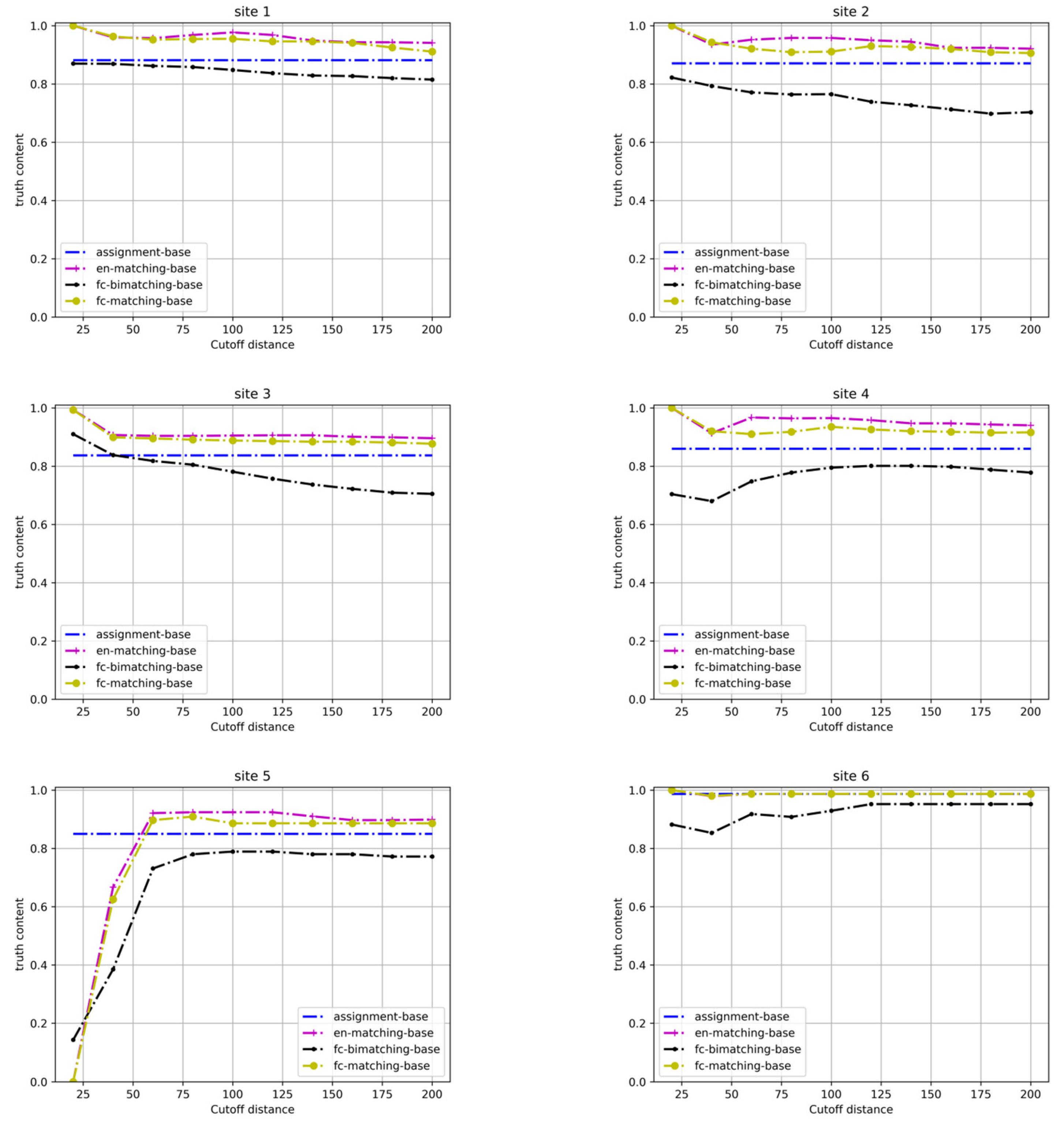
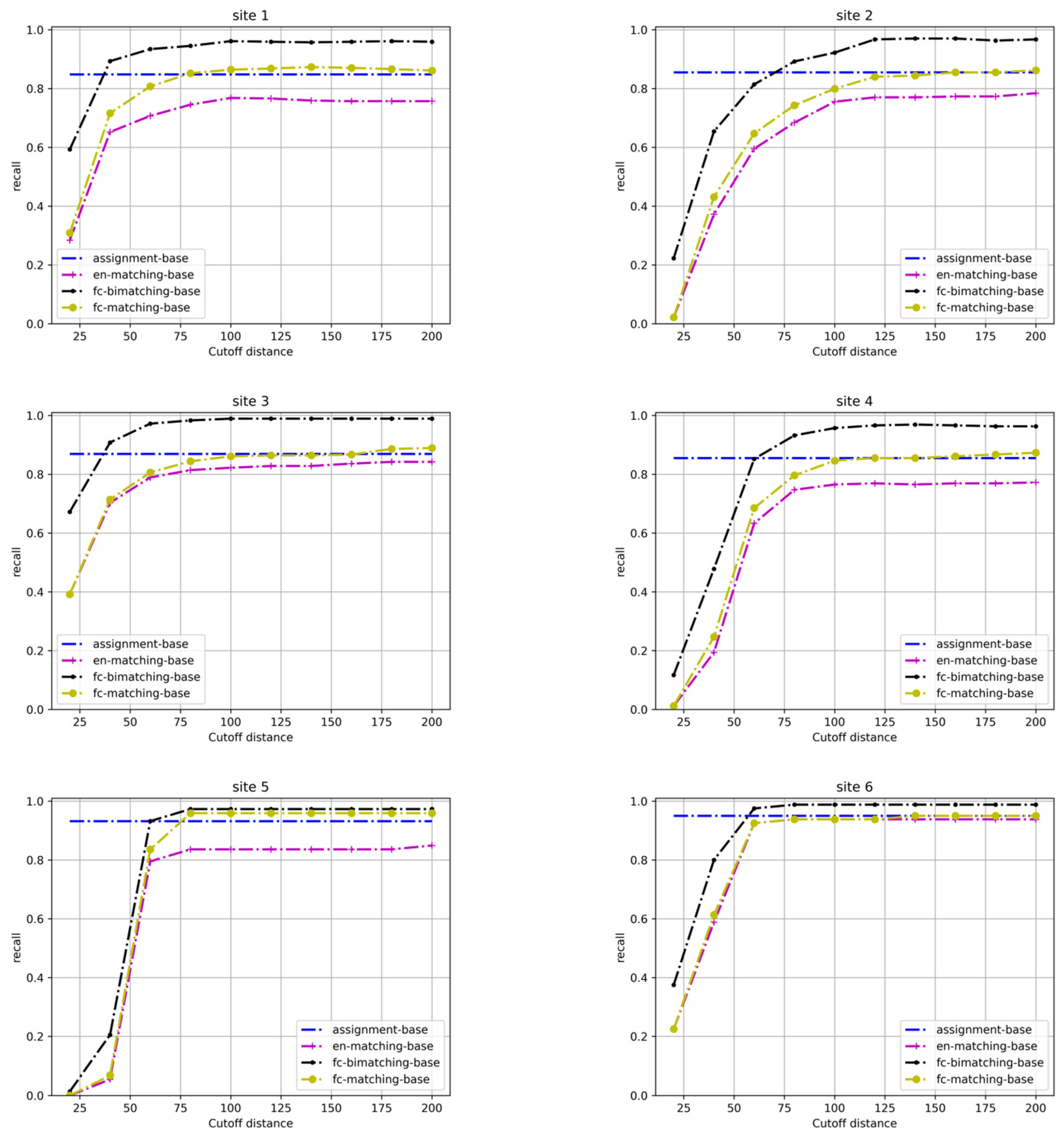
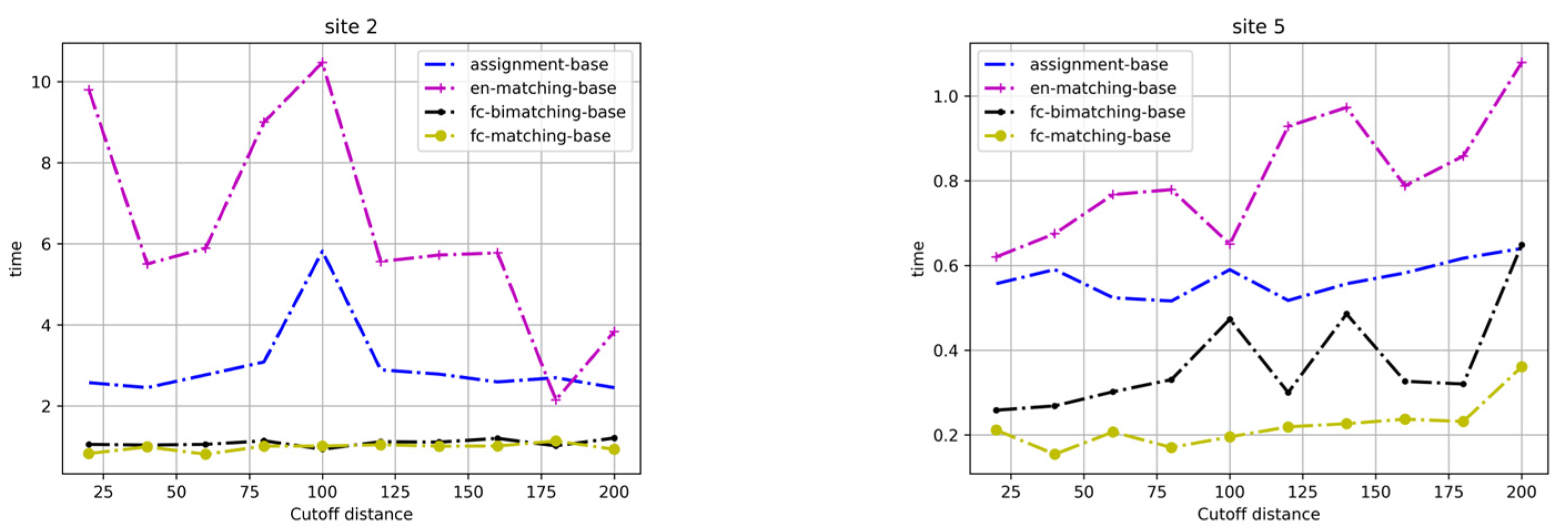
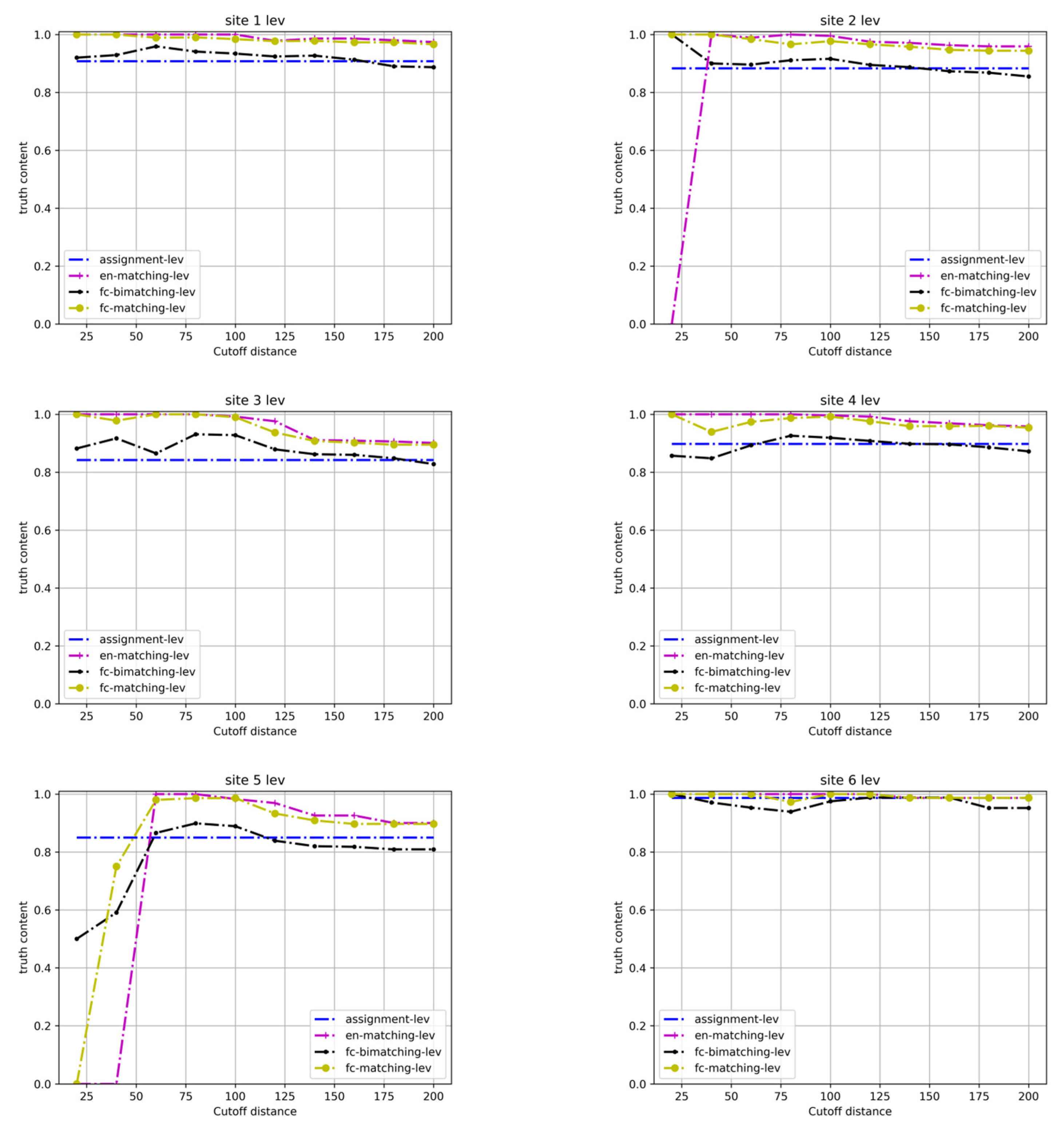
4.2. Experimental Results

We tested the proposed en-matching model and the main existing optimized conflation models in the literature, including the assignment problem and the fixed-charge matching models on the Santa Barbara test sites. For the model parameters, we chose $\beta$ to be 4, assuming four roads per street intersection, as discussed earlier. We chose $\gamma$ to be 0.5. Setting $\gamma =0$ causes the disconnected components problem, whereas larger $\gamma$ values do not seem to improve the performance. The most sensitive parameter was the cut-off distance $c$. As covered in the Background section, early TIGER/Line roads can have large spatial displacements amounting to 85.7 m in terms of the median distance when compared to GPS measurements [25]. The OSM data can also have spatial displacement (although probably smaller displacement, as it is more recent). Therefore, we tested a range of cut-off distances from 20–200 m at 20 m intervals. We chose 100 m as a typical cut-off distance. The distances between features are measured in terms of the Hausdorff distance (and the directed Hausdorff distance for fc-bimatching problem), as explained in the Background section.

Precision

Figure 5 presents the precision rates of the tested models under different cut-off distances. For all tested models, we can observe a clear downward trend for precision as the cut-off distance increases for all models except the assignment model. This is because, at very small cut-off distances, only very close features are allowed in the match, and the chances of making false matches are low. As the cut-off distance increases, more ambiguous candidate feature pairs are considered; hence, the precision is lower. The assignment model is not controlled by the cut-off distance, as it requires all features to be matched. Among the four optimized conflation models, the fc-bimatching model achieves the lowest precision. As discussed earlier, this is because the fc-bimatching model is the only tested model that allows many-to-one matches. Many-to-one matches are more noisy, and their logical consistency is more difficult to enforce with logical conditions. The other three models are one-to-one conflation models (assuming equality relation in matching). They cannot capture many-to-one matches at all, but they capture one-to-one matches with higher certainty, as shown in the figure. Among the three one-to-one models, the new en-matching model consistently achieves the highest precision. The assignment model achieves the lowest precision in the one-to-one models. At a cut-off distance of 100 m, the en-matching, fc-matching, assignment, and fc-bimatching formulations achieved average precisions of 95.3%, 92.7%, 88.1%, and 81.8%, respectively, across the six test sites. Although the precision of the fc-matching model was already high, the new model improved the precision by 2.8%. This is likely due to the node-arc relations enforced by the en-matching model ruling out some false matches.

Recall

Figure 6 presents the recall rates of the tested models on the Santa Barbara dataset. Unlike the precision curves in Figure 5, Figure 6 shows a clear upward trend for recall as the cut-off distance increases (except for the assignment model). This is because, with greater cut-off distances, more distant pairs of features are admitted into the matching process. These include both true and false matches, which is why the precision drops (Figure 5) while recall increases (Figure 6). There is also a clear difference between the many-to-one conflation model fc-bimatching and the one-to-one models, with the former having significantly higher recall rates. This is because one-to-one models miss all partial matches via construction. Generally, the recall rate saturates after the cut-off distance is 100 m or greater, indicating that most of the true matches are in this range. On average, the fc-bimatching, assignment, fc-matching, and en-matching models achieved recall rates of 96.5%, 88.5%, 87.8%, and 81.4%, respectively. The proposed en-matching model has the lowest rate of admittance, but it still captures over 81% of the true matches.

Computational time

Figure 7 presents the computational time of the tested models on the Santa Barbara dataset. For reasons of spatial restriction, we only present the computational times for site 2 (which took the longest time) and site 5 (which took the shortest time). From the figure, the new en-matching model consistently took longer (computational time) despite some fluctuations. At site 2, with a cut-off distance of 100 m, the new node-arc model took 10.5 s to solve the process; the assignment model took 5.8 s, whereas the network-flow-based fc-matching and fc-bimatching models took 1 and 0.9 s, respectively. At site 5, with a 100 m cut-off, the same four models took 0.7, 0.6, 0.2, and 0.5 s, respectively. The network-flow-based models are faster because the underlying network flow problem, in general, has a lower computational complexity than integer linear programming (ILP). While both the en-matching and assignment models are formulated in ILP, the new en-matching model took longer, presumably because it has a more complex constraint structure than the assignment model.

Considering the size of the tested sites, the computational times are still acceptable. However, practical road networks are much larger. This means that the worst-case computational time can increase rapidly as the data size increases. In order to cope with this potential scalability issue, one can employ a divide-and-conquer strategy and divide the network into overlapping blocks. The node-arc model can then be applied within each block to match features. This process requires asymmetric buffering around the blocks to include periphery shapes from neighboring blocks. The interested reader is referred to [35] for a detailed description of the divide-and-conquer process and different partitioning strategies.

Models Enhanced with String Distances

We also tested an enhanced version of each tested model in which the between-feature distance was computed as the weighted sum of the basic (directed) Hausdorff distance and a string distance between the street names. We adopted the widely used Levenshtein distance to measure string dissimilarity (ranging from 0 to 1.0). We then multiplied the Levenshtein distance by 100 and added it to the Hausdorff distance to form a composite distance metric. By using a composite distance, this implies that we are penalizing feature pairs (both streets and junctions) with dissimilar names. In calculating the string distance, we removed redundant whitespaces, as mentioned earlier, and concatenated the names of all streets meeting at a given junction as the names of the junction.

Precision

Figure 8 presents the precision rates for the enhanced models on the same Santa Barbara dataset. We can observe a similar general trend of lower precision with higher cut-off distances. However, the precision rates for all models increased to higher levels with the enhanced distance metric. The proposed en-matching model consistently outperforms all other models, although the performance advantage becomes smaller as other models, such as the ec-matching model, achieve near-perfect precision with the enhanced distance. On average, the en-matching, fc-matching, assignment, and fc-bimatching models achieved precisions of 99.4%, 98.8%, 89.5%, and 92.7%, respectively.

Recall

Improved precision is expected by incorporating names. However, it comes at the cost of lower recall rates. Figure 9 presents the recall rates of the enhanced models under various cut-off distances. In addition to the same general trend of higher recall with larger cut-off distances, we can observe that the proposed en-matching model has the lowest recall among all models. On average, the recall rates of the fc-bimatching, assignment, fc-matching, and en-matching models are 94.7%, 89.8%, 85%, and 74.7%, respectively. These rates are 1.8%, −1.3%, 2.8%, and 5.8% lower than those of the original versions of the models, respectively. We can observe that while enhancing the models with string distance improved precision, the recall rates are generally lower, with the proposed en-matching model being the most impacted. This lower rate is presumably because the junction names may be problematic for string distances. For example, if a road junction is represented as a four-way junction in one dataset but as a T-junction in another (e.g., due to a missing road), then the junction names will differ by 25% on average. This will incur a large string distance or penalty, which may result in the junction pair being unmatched. Moreover, the node-arc constraints (6) through (9) prevent all roads incident to the junction in question from being matched. In this case, using string distance can rule out multiple edges around a junction because the string distance incorrectly indicates that there is no match at the junction itself.

Finally, we tested the sensitivity of the $\gamma$ parameter. Although it does improve some specific cases (as shown in Section 3), the overall effect is not significant. We found only a marginal improvement in recall and precision when $\gamma$ was increased from 0 to 0.5. Larger $\gamma$ values at 1.0 and 1.5 do not improve or degrade the performance.

5. Conclusions and Future Directions

Spatial data conflation is a widely needed yet complex task that has been a barrier to many types of spatial analyses for decades. One of the main issues of geospatial conflation is the unreliability of the automatic conflation methods. Due to spatial displacement, different levels of detail and representation, and other factors in the cartographic process, conflation algorithms can often be misled and produce false matches. Therefore, computerized conflation methods are often deemed untrustworthy and require heavy human intervention and correction. Traditional conflation methods rely heavily on measuring the similarity between individual feature pairs and matching the feature pairs that are the most similar or closest. These methods are often greedy in nature and may result in erroneous or even conflicting matches. Optimized conflation methods overcome much of this greediness, yet they are somewhat weak at present. As discussed in the literature review, most of the model constructs in the existing models of optimized conflation are related to cardinality relations.

This study addresses the unreliability of optimized conflation by introducing a node-arc topology into the matching process. In particular, we propose a new edge-node matching model (en-matching) that simultaneously matches the edges and nodes of two network datasets (such as road or river networks). We impose logical constraints that force the model to match the edges and nodes in a manner that respects the topological relation between the nodes and edges. This construct prevents inconsistent matches and increases the reliability of automatic conflation. We also tested the possibility of using string distances between the names of street junctions (and streets) to further reduce false matches. In a sense, the new en-matching model automates the well-known rubber-sheeting method by treating all network junctions as anchor points and then matching them together with the connected edges in a spatially consistent manner.

Our experiments on the Santa Barbara road networks [27,30] show that the proposed en-matching model is more selective. It achieved an average precision of 95.3%, which was 2.8% higher than that of the second-best model (fc-matching) over the six test sites. This means that the truth content of the en-matching is higher. Meanwhile, as a more conservative model, the en-matching model missed more true matches. It achieved a recall rate of 81.4%, which is 6.4% lower than that of the fc-matching model. In the context of conflation, a higher precision is presumably more important because all models can already capture over 80% of the true matches. Checking for errors in a large number of computer-generated matches is more costly than matching a small number of unmatched features untouched by the computer. We also found that by employing a string distance (Levenshtein) between street names and between junction names, the precision of the new model could be improved to 99.4%, while the recall further dropped to 74.7%. This means that only 1 in 200 matches is incorrect, and the human expert has to match the remaining one-quarter of the roads (many of them partial matches, presumably).

The relatively lower recall rate is partly due to the fact that the en-matching model is a one-to-one matching model. As with the two other one-to-one models, the en-matching model cannot capture any partial matches. Additional modeling constructs need to be developed to complement the en-matching model and handle partial matches. This is left for future research. Another possible direction for future work is to explore the use of other string distances. Adding the Levenshtein distance brought precision to a near-perfect level yet caused the recall rate to drop by 5.7%. It is worthwhile to test the many other string distances in the literature to determine whether they can perform better. Yet another future direction is to improve the tooling of conflation to ease the adoption of the new model by GIS practitioners. This includes, e.g., the development of a user-friendly interface for applying the model, a user interface for the manual correction of mismatches, and additional tools/logic for the subsequent attribute merging/transfer stage based on the model-generated match.

References

1. Rosen, B.; Saalfeld, A. Match Criteria for Automatic Alignment. In Proceedings of the 7th International Symposium on Computer-Assisted Cartography (Auto-Carto 7), Washington, DC, USA, 11–14 March 1985; pp. 1–20. [Google Scholar]
2. Saalfeld, A. Conflation automated map compilation. Int. J. Geogr. Inf. Syst. 1988, 2, 217–228. [Google Scholar] [CrossRef]
3. Cobb, M.A.; Chung, M.J.; Iii, H.F.; Petry, F.E.; Shaw, K.B.; Miller, H.V. A rule-based approach for the conflation of attributed vector data. GeoInformatica 1998, 2, 7–35. [Google Scholar] [CrossRef]
4. Filin, S.; Doytsher, Y. Detection of corresponding objects in linear-based map conflation. Surv. Land Inf. Syst. 2000, 60, 117–128. [Google Scholar]
5. Masuyama, A. Methods for detecting apparent differences between spatial tessellations at different time points. Int. J. Geogr. Inf. Sci. 2006, 20, 633–648. [Google Scholar] [CrossRef]
6. Pendyala, R.M. Development of GIS-Based Conflation Tools for Data Integration and Matching; Florida Department of Transportation: Lake City, FL, USA, 2002.
7. Ruiz, J.J.; Ariza, F.J.; Ureña, M.A.; Blázquez, E.B. Digital map conflation: A review of the process and a proposal for classification. Int. J. Geogr. Inf. Sci. 2011, 25, 1439–1466. [Google Scholar] [CrossRef]
8. Xavier, E.M.A.; Ariza-López, F.J.; Ureña-Cámara, M.A. A survey of measures and methods for matching geospatial vector datasets. ACM Comput. Surv. 2016, 49, 1–34. [Google Scholar] [CrossRef]
9. MacEachren, A.M. Compactness of geographic shape: Comparison and evaluation of measures. Geogr. Ann. Ser. B Hum. Geogr. 1985, 67, 53–67. [Google Scholar] [CrossRef]
10. Zhang, X.; Zhao, X.; Molenaar, M.; Stoter, J.; Kraak, M.-J.; Ai, T. Pattern classification approaches to matching building polygons at multiple scales. ISPRS Ann. Photogramm. Remote Sens. Spat. Inf. Sci. 2012, 1, 19–24. [Google Scholar] [CrossRef]
11. Tang, W.; Hao, Y.; Zhao, Y.; Li, N. Research on areal feature matching algorithm based on spatial similarity. In Proceedings of the 2008 Chinese Control and Decision Conference, Yantai, China, 2–4 July 2008; pp. 3326–3330. [Google Scholar]
12. Tong, X.; Shi, W.; Deng, S. A probability-based multi-measure feature matching method in map conflation. Int. J. Remote Sens. 2009, 30, 5453–5472. [Google Scholar] [CrossRef]
13. Wentz, E.A. Shape Analysis in GIS. In Proceedings of the Auto-Carto, Seattle, WA, USA, 7–10 April 1997; Volume 13, pp. 7–10. [Google Scholar]
14. Eiter, T.; Mannila, H. Computing discrete fréchet distance. Citeseer 1994. [Google Scholar]
15. Chambers, E.W.; De Verdiere, E.C.; Erickson, J.; Lazard, S.; Lazarus, F.; Thite, S. Homotopic fréchet distance between curves or, walking your dog in the woods in polynomial time. Comput. Geom. 2010, 43, 295–311. [Google Scholar] [CrossRef]
16. Arkin, E.M.; Chew, L.P.; Huttenlocher, D.P.; Kedem, K.; Mitchell, J.S. An Efficiently Computable Metric for Comparing Polygonal Shapes; Cornell University: Ithaca, NY, USA, 1991. [Google Scholar]
17. Lei, T.L.; Wang, R. Conflating linear features using turning function distance: A new orientation-sensitive similarity measure. Trans. GIS 2021, 25, 1249–1276. [Google Scholar] [CrossRef]
18. Harvey, F.; Vauglin, F.; Ali, A.B.H. Geometric matching of areas, comparison measures and association links. In Proceedings of the 8th International Symposium on Spatial Data Handling, Vancouver, BC, Canada, 11–15 July 1998; pp. 557–568. [Google Scholar]
19. Huh, Y.; Yu, K.; Heo, J. Detecting conjugate-point pairs for map alignment between two polygon datasets. Comput. Environ. Urban Syst. 2011, 35, 250–262. [Google Scholar] [CrossRef]
20. Fan, H.; Zipf, A.; Fu, Q.; Neis, P. Quality assessment for building footprints data on OpenStreetMap. Int. J. Geogr. Inf. Sci. 2014, 28, 700–719. [Google Scholar] [CrossRef]
21. Goodchild, M.F.; Hunter, G.J. A simple positional accuracy measure for linear features. Int. J. Geogr. Inf. Sci. 1997, 11, 299–306. [Google Scholar] [CrossRef]
22. Li, L.; Goodchild, M.F. Optimized feature matching in conflation. In Proceedings of the Geographic Information Science: 6th International Conference, GIScience, Zurich, Switzerland, 14–17 September 2010; pp. 14–17. [Google Scholar]
23. McKenzie, G.; Janowicz, K.; Adams, B. A weighted multi-attribute method for matching user-generated points of interest. Cartogr. Geogr. Inf. Sci. 2014, 41, 125–137. [Google Scholar] [CrossRef]
24. Liadis, J.S. GPS TIGER accuracy analysis tools (GTAAT) evaluation and test results. US Bur. Census Div. Geogr. TIGER Oper. Branch 2000. [Google Scholar]
25. Zandbergen, P.A.; Ignizio, D.A.; Lenzer, K.E. Positional Accuracy of TIGER 2000 and 2009 Road Networks. Trans. GIS 2011, 15, 495–519. [Google Scholar] [CrossRef]
26. Church, R.; Curtin, K.; Fohl, P.; Funk, C.; Goodchild, M.F.; Kyriakidis, P.; Noronha, V. Positional distortion in geographic data sets as a barrier to interoperation. In Proceedings of the ACSM Annual Convention, Baltimore, MD, USA, 27 February–5 March 1998. [Google Scholar]
27. Lei, T.L. Geospatial data conflation: A formal approach based on optimization and relational databases. Int. J. Geogr. Inf. Sci. 2020, 34, 2296–2334. [Google Scholar] [CrossRef]
28. Beeri, C.; Kanza, Y.; Safra, E.; Sagiv, Y. Object fusion in geographic information systems. In Proceedings of the Thirtieth International Conference on Very Large Data Bases, Toronto, ON, Canada, 31 August–3 September 2004; Volume 30, pp. 816–827. [Google Scholar]
29. Hillier, F.S.; Lieberman, G.J. Introduction to Operations Research, 8th ed.; McGraw-Hill: New York, NY, USA, 2005; p. 1088. [Google Scholar]
30. Li, L.; Goodchild, M.F. An optimisation model for linear feature matching in geographical data conflation. Int. J. Image Data Fusion 2011, 2, 309–328. [Google Scholar] [CrossRef]
31. Tong, X.; Liang, D.; Jin, Y. A linear road object matching method for conflation based on optimization and logistic regression. Int. J. Geogr. Inf. Sci. 2013, 28, 824–846. [Google Scholar] [CrossRef]
32. Lei, T.; Lei, Z. Optimal spatial data matching for conflation: A network flow-based approach. Trans. GIS 2019, 23, 1152–1176. [Google Scholar] [CrossRef]
33. Revelle, C.; Marks, D.; Liebman, J.C. An Analysis of Private and Public Sector Location Models. Manag. Sci. 1970, 16, 692–707. [Google Scholar] [CrossRef]
34. ReVelle, C. Facility siting and integer-friendly programming. Eur. J. Oper. Res. 1993, 65, 147–158. [Google Scholar] [CrossRef]
35. Lei, T.L. Large scale geospatial data conflation: A feature matching framework based on optimization and divide-and-conquer. Comput. Environ. Urban Syst. 2021, 87, 101618. [Google Scholar] [CrossRef]
Figure 1. A hypothetical example of a node-arc match relation. A green arrow (urs) indicates a nodal match from nodes r to s; a blue arrow (xij) indicates an edge match from edges i to j.
Ijgi 13 00015 g001
Figure 2. Connectivity gap at test site 1 when matching the Santa Barbara road networks from Open Street Map (green) and TIGER (red) without the degree term in the objective.
Ijgi 13 00015 g002
Figure 3. Six tested road datasets in Santa Barbara County, CA: Open Street Map (green) and TIGER (red).
Ijgi 13 00015 g003
Figure 4. Labeling ground truth for matching with node-arc topology.
Ijgi 13 00015 g004
Figure 5. Precision of conflation models for the Santa Barbara road networks (OSM vs. TIGER).
Ijgi 13 00015 g005
Figure 6. Recall of conflation models for the Santa Barbara road networks (OSM vs. TIGER).
Ijgi 13 00015 g006
Figure 7. Computation times (s) of conflation models for the Santa Barbara road networks (OSM vs. TIGER, sites 2 and 5).
Ijgi 13 00015 g007
Figure 8. Precision of enhanced conflation models (with Levenshtein distance) on the Santa Barbara road networks.
Ijgi 13 00015 g008
Figure 9. Recall of enhanced conflation models (with Levenshtein distance) on the Santa Barbara road networks.
Ijgi 13 00015 g009
Disclaimer/Publisher’s Note: The statements, opinions and data contained in all publications are solely those of the individual author(s) and contributor(s) and not of MDPI and/or the editor(s). MDPI and/or the editor(s) disclaim responsibility for any injury to people or property resulting from any ideas, methods, instructions or products referred to in the content.