Abstract
The pursuit of the Sustainable Development Goals has highlighted rural electricity consumption patterns, necessitating innovative analytical approaches. This paper introduces a novel method for predicting rural electricity consumption by leveraging deep convolutional features extracted from satellite imagery. The study employs a pretrained remote sensing interpretation model for feature extraction, streamlining the training process and enhancing the prediction efficiency. A random forest model is then used for electricity consumption prediction, while the SHapley Additive exPlanations (SHAP) model assesses the feature importance. To explain the human geography implications of feature maps, this research develops a feature visualization method grounded in expert knowledge. By selecting feature maps with higher interpretability, the “black-box” model based on remote sensing images is further analyzed and reveals the geographical features that affect electricity consumption. The methodology is applied to villages in Xinxing County, Guangdong Province, China, achieving high prediction accuracy with a correlation coefficient of 0.797. The study reveals a significant positive correlations between the characteristics and spatial distribution of houses and roads in the rural built environment and electricity demand. Conversely, natural landscape elements, such as farmland and forests, exhibit significant negative correlations with electricity demand predictions. These findings offer new insights into rural electricity consumption patterns and provide theoretical support for electricity planning and decision making in line with the Sustainable Development Goals.
1. Introduction
In 2015, the United Nations included energy as one of the 17 Sustainable Development Goals (SDGs) in the 2030 Agenda for Sustainable Development [1]. SDG 7.1 aims to ensure access to affordable, reliable, and modern energy services for all [2,3]. According to official SDG 7.1.1 data, about 789 million people lacked access to electricity in 2018 [4]. However, these statistics are aggregated at the national level [5], making it difficult to understand the distribution of this population on a finer spatial scale, especially in data-scarce rural areas, thereby hindering further humanitarian aid planning [6]. Therefore, there is a lack of fine-scale, global electricity data and measurement methods related to SDG 7.1.
The integration of satellite imagery and machine learning (SIML) has opened up a significant area for the application of AI to remotely estimate the socio-economic and environmental conditions of data-scarce regions to address global challenges [6,7,8,9]. Over the past two decades, there has been a rapid increase in the development and application of various machine learning models in energy systems [10,11]. A systematic review of 70 journal articles published between 2015 and 2018 on building energy performance prediction found that 61% of the studies focused on individual buildings, while 39% focused on the urban scale [12]. These studies heavily relied on data-driven approaches, utilizing data on building characteristics, occupants, and climate to predict energy efficiency and consumption patterns [13,14,15]. Furthermore, satellite remote sensing imagery is increasingly being applied in energy consumption forecasting [16,17,18]. Currently, the remote sensing field primarily uses nighttime light satellite imagery to estimate electricity consumption [19,20,21,22]. For example, Elvidge et al. estimated electricity consumption using radiance-calibrated images extracted from DMSP/OLS low-light nighttime images captured from 1996 to 1997, noting that these images can be used to accurately estimate electricity consumption [23,24].
This is particularly relevant in rural areas with scarce data. But can satellite remote sensing imagery be used to accurately determine electricity consumption levels in these regions [25]? Rural areas are relatively dispersed, and nighttime light data often lack sufficient accuracy in these regions, leading to significant variability and fluctuations. However, many small rural communities and individual households, both in developed and developing countries, do not generate detectable levels of nighttime radiation by satellites [26]. This limits the application of nighttime light data on a fine scale in rural areas [27,28].
Daytime satellite imagery can clearly record geographic elements resulting from human activities [29,30]. Human socio-economic activities inevitably lead to changes in geology and geomorphology, forming corresponding geographic elements, such as buildings, farmlands, roads, etc., which can reflect the socio-economic status of settlements, such as poverty [6,7,8]. Can daytime satellite imagery reflect average levels of electricity consumption and which geographic elements in the imagery are related to it [31,32]? Currently, there is almost no relevant research revealing these relationships.
The explainable artificial intelligence (XAI) aspect of SIML might answer this question [33], which is also a core challenge in SIML development, i.e., explainability [34]. The development of machine learning, especially deep learning, has made AI models increasingly complex and powerful, but these models have become more opaque [35]. The research direction of XAI aims to make machine learning models capable of providing explanations in terms understandable to humans [36]. It is proposed that through SIML methods, users can fit various socio-economic and environmental attributes globally [37], such as income levels, population density, and forest cover, and achieve good fitting results [8]. Deep convolutional features are highly effective at capturing complex spatial patterns in satellite imagery, which are strongly correlated with electricity consumption [38]. For example, factors like building density and land use type significantly impact energy consumption. Through automated feature extraction, convolutional neural networks can learn nonlinear relationships from this spatial data [39]. Moreover, the widespread use of deep learning in energy forecasting further demonstrates its effectiveness in tasks similar to predicting electricity consumption [40,41]. However, there is no suitable XAI in the SIML field that can effectively explain the relationships between deep convolutional features and the topics of interest.
Consequently, an innovative explainable SIML approach is designed for predicting village-level average electricity consumption using satellite remote sensing deep feature maps. Furthermore, it endeavors to establish and elucidate the relationships among these elements from a rural planning perspective. Rural buildings are the most important assets for a rural household, reflecting the social–economic status of the rural area to a great extent [42,43]. The pretrained Mask R-CNN model, which specializes in building-footprint extraction, is employed to generate feature maps of various geographic elements from high-resolution satellite imagery [44]. It is hypothesized that the feature maps are highly related to household electricity consumption. Thus, a random forest model is constructed to relate feature values to electricity consumption levels, and the SHapley Additive exPlanations (SHAP) is used to identify the most critical features and explain their meanings and relationships [45].
The main innovations and contributions of this paper can be summarized as follows: First, this study designed an innovative framework for the prediction and interpretation of electricity consumption using high-resolution remote sensing images. Subsequently, remote sensing image features were extracted as explanatory variables, but these features contained a lot of redundant information. Therefore, this paper used the SHAP model to screen for the most important features that explain electricity consumption. To further explain the geographical significance of these features, expert knowledge and visual feature maps were employed to interpret the extracted features. Finally, the correlations between key geographical features and electricity consumption were analyzed, and these features were used to predict electricity consumption levels.
2. Data and Methods
This study takes the electricity consumption of villages in Xinxing County, Guangdong Province, as a case study. It uses the feature pyramid network (FPN) from a Mask RCNN model trained on previous work to generate a series of feature maps from daytime satellite imagery and establishes a regression relationship between these feature maps and village electricity consumption to interpret them in terms of human geography. This section explains the core data, principles of FPN, and basic technical framework.
2.1. Case Area and Data
2.1.1. Case Area
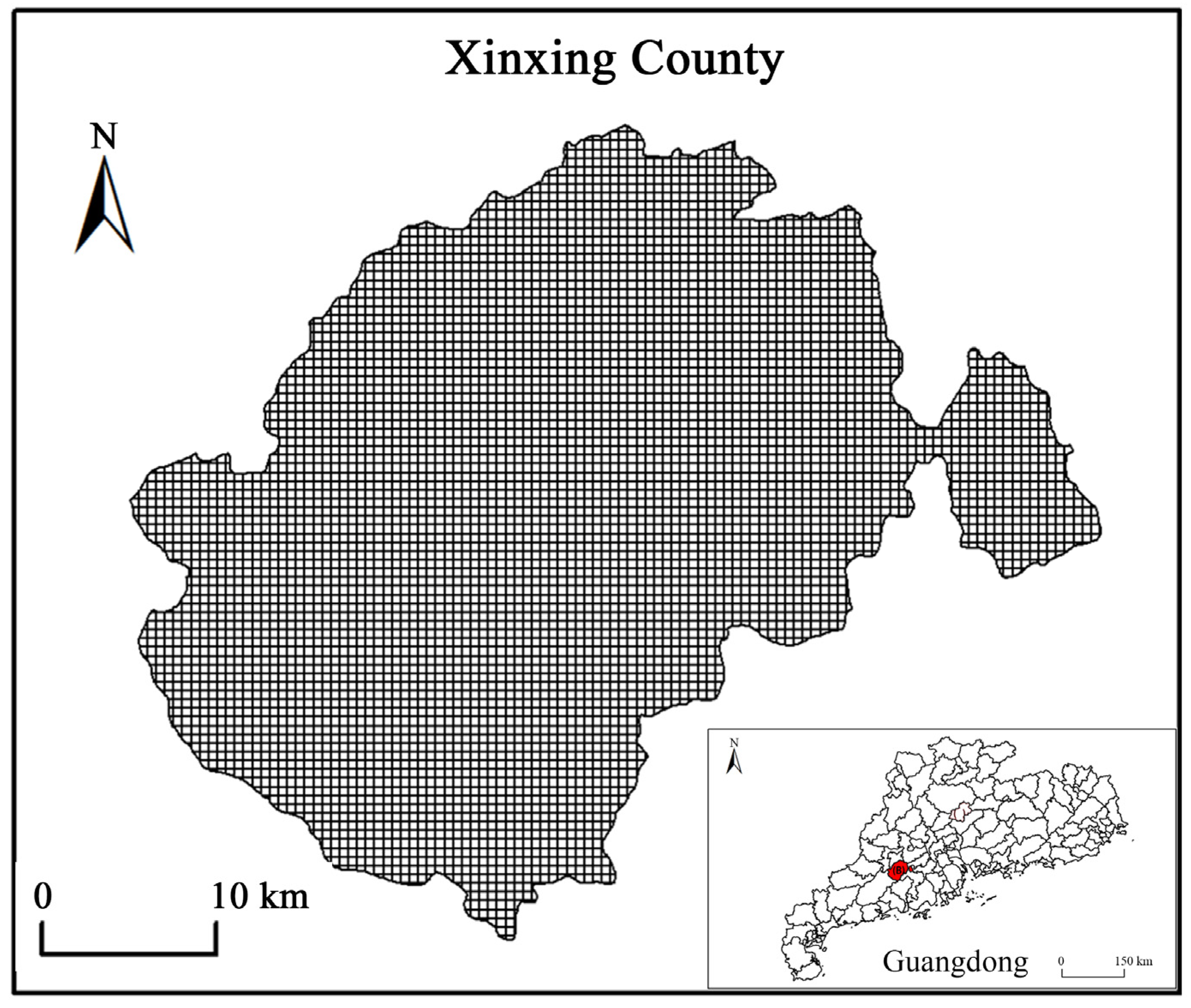
Xinxing County is located in the central western part of Guangdong Province, China (Figure 1). It is 58 km (about one hour’s drive) from the urban area of Yunfu city and more than 130 km (1.5 hours’ drive) from Guangzhou. It has several highways and roads connecting it to the outside, placing it within a 2 h transportation circle of the Pearl River Delta.
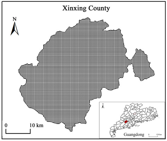
Figure 1.
The location of Xinxing County in Guangdong.
Xinxing County is a typical mountainous agricultural county. Surrounded by mountains, it features a topography that is higher in the south and lower in the north. Rivers form several narrow and wide valley areas, where fertile soil, sufficient light and heat make it very suitable for agricultural cultivation. The income level of rural residents in Xinxing County is relatively high. The income level of rural residents in Xinxing County is relatively high. In 2021, the per capita disposable income of rural residents reached CNY 21,983. As of 2021, 43% of the population still lived in rural areas.
To analyze electricity consumption patterns and spatial characteristics, a fishnet grid of 500 m × 500 m was superimposed on the area (Figure 1). Each grid cell represented an aggregated spatial unit for electricity consumption data, allowing us to examine the distribution of energy use at the village level while maintaining consistency with the satellite imagery. This grid-based approach enables detailed spatial analysis of rural development patterns, helping to identify key areas of high or low electricity consumption, which may correlate with factors such as household density, infrastructure quality, or economic activity.
2.1.2. Village Electricity Data
The electricity consumption data used in this study were obtained from China Southern Power Grid Company Limited, with all data collected for the year 2021. In recent years, Southern Power Grid has been strengthening the construction of rural digital power grids in Guangdong Province, capable of collecting monthly household electricity consumption for each meter, with detailed spatial location information. Generally, meters are attached to farmhouses, and the level of electricity usage may be visible for farmhouses or the entire village environment. For example, new farmhouses may have higher levels of electricity consumption.
For user privacy and confidentiality, household electricity consumption was aggregated into 500 m × 500 m grids, representing the village scale. Average electricity consumption was calculated by averaging the annual household electricity consumption within the grid, excluding any individual-scale information. Additionally, random disturbances were added to the average electricity consumption to obscure the exact amount of electricity used, so the data only represent the average electricity level of a 500 m × 500 m grid.
Since this study focuses on village development and planning, grids with a building-to-area ratio of less than 10% were filtered out using a building extraction algorithm. Ultimately, 547 grids (villages) of 500 m × 500 m were used in this study.
2.1.3. Remote Sensing Data
The remote sensing data used in this study are high-resolution images from Google Earth, collected in 2021 to ensure alignment with the electricity consumption data. These data consist of tile images that comprise red, green, and blue spectral bands, with a spatial resolution of 0.25 m. This level of detail renders the images highly discernible and interpretable to the human eye. The 547 grids (villages) used for electricity data were matched with their corresponding remote sensing tiles, ensuring consistency in both space and time for the analysis.
2.2. Pretrained Mask R-CNN for Feature Extraction
Buildings are widely recognized as one of the most intuitive indicators of electricity consumption. To extract image features related to buildings, this study employed a Mask R-CNN model [46], which was trained on a diverse dataset of 15,000 labeled samples collected from across the country, serving as the foundational framework [23]. The national model of this framework demonstrates impressive performance, achieving an accuracy of 0.776, a recall of 0.755, and an F1 score of 0.765. These outstanding metrics indicate that the model has successfully captured and extracted deep features related to buildings. Through SHAP analysis, we evaluated the importance of the features within the FPN and elucidated the practical significance of key features and their correlation with electricity consumption.
FPN is a method for extracting multiscale feature maps by constructing pyramid structures, allowing for the extraction of features from targets of different scales [47]. In traditional feature extraction, images undergo convolution and pooling, obtaining low-level features such as edges, textures, and colors in shallow networks [48,49], while deeper networks obtain more abstract semantic features used for target classification and segmentation. However, these networks have single-scale features, making them unsuitable for images with multiscale targets. For dense, small targets, details are easily lost after multiple convolutions, leading to poor detection performance. The use of different levels of feature maps directly for prediction, although achieving multiscale prediction ability, lacks the integration of feature maps [50,51]. Shallow feature maps retain a large amount of information for predicting small targets [52], such as shapes and edges, but lack semantic information, leading to misclassification.
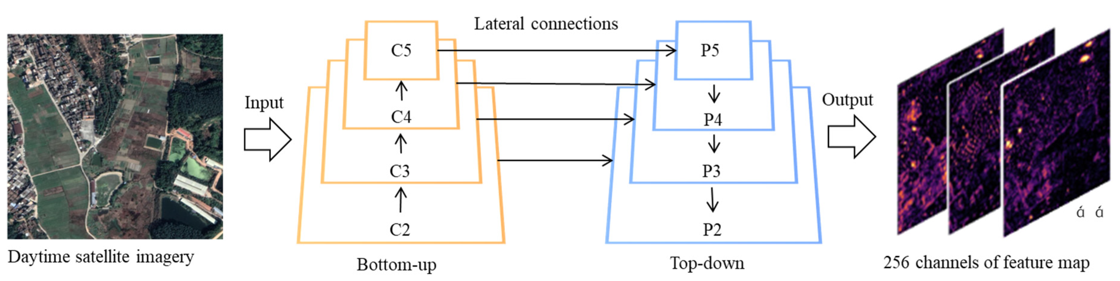
FPN addresses the above problems by allowing deep feature maps to merge with shallower feature maps, causing lower feature maps to retain their shape characteristics, like edges, textures, and colors, while also containing deep semantic information. Through the pyramid structure, the network can process targets or image features on different scales simultaneously. Lower feature maps correspond to smaller targets or local details, while top feature maps correspond to larger targets or global semantic information. The network can select appropriate feature maps based on specific tasks. Overall, the process of generating feature maps can be divided into bottom-up and top-down processes (Figure 2).
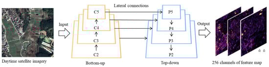
Figure 2.
Feature pyramid work flowchart.
Bottom-Up Process: This process is the forward process of traditional convolutional neural networks, extracting image features through five stages, with the last feature map of each stage as the final output, forming the feature pyramid. For Mask R-CNN models, ResNet is mainly used. The feature activation of the last residual structure of each stage is used as the feature map output. As shown in the figure, the output modules were {C2, C3, C4, C5}, corresponding to the outputs of conv2, conv3, conv4, and conv5. These feature maps contain deep and abstract semantic information on remote sensing images.
Top-Down Process: By interpolating the feature map of the upper layer, the size was increased to match the size of the next layer feature map. Then, a 1 × 1 convolution operation was performed on the corresponding feature map from the side and merged with the upsampled feature map, forming new feature maps. Finally, a 3 × 3 convolution kernel was used to convolve the new feature maps to generate the {P2, P3, P4, P5} feature maps. These feature maps possess both abstract semantic information and high-resolution spatial information of remote sensing images. The P series feature maps were ultimately used for target detection tasks.
The final feature maps show spatial differentiation of high and low values. High-value areas are positive activation areas, indicating that the network has detected the target or feature of interest at that position or channel. Low-value areas are negative activation areas, indicating that the target or feature of interest was not found at that position. The boundary between positive and negative is usually zero or the average value. This study used the average value to distinguish between positive and negative activation areas and positively activated areas as the main feature inputs to study their relationships with electricity consumption.
2.3. Framework for Electricity Forecasting and Feature Interpretability
This study proposes an explainable regression (XRegression) framework to understand the geographic elements in satellite imagery and establish relationships with average electricity consumption levels, achieving electricity prediction and explanation. XRegression includes the following three steps (Figure 3):
- (1)
- Feature maps extraction: this step uses a Mask R-CNN model to extract building features from satellite images, using the FPN to obtain feature maps with clear spatial and high-level semantic information and convert them into deep convolutional features.
- (2)
- Feature maps selection: this step uses a random forest model to establish mapping relationships among variables, then uses the SHAP model to filter a small number of key explanatory features, facilitating the interpretation of the relationship between independent and dependent variables.
- (3)
- Feature maps explanation and electricity prediction: this step explores the geographic connotations of key features by feature visualization and combines rural planning expertise to analyze their relationships with electricity consumption.
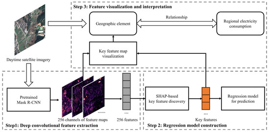
Figure 3.
Flowchart of the electricity forecasting and feature explanation analysis.
Figure 3.
Flowchart of the electricity forecasting and feature explanation analysis.

- Step 1: Deep Convolutional Feature Extraction
This step is aimed at extracting clear deep convolutional feature maps containing geographic element information from satellite imagery. Deep learning models generally produce deep convolutional features through the network backbone. The Mask R-CNN model used the ResNet + FPN combination structure, representing deep convolutional features in a pyramid form (Figure 2), providing deep convolutional feature information for subsequent target detection and semantic segmentation functions. FPN involves bottom-up pathways, top-down pathways, and lateral connections. The bottom-up pyramid {C2, C3, C4, C5} represents the outputs of conv2, conv3, conv4, and conv5, with semantic information increasing from low to high, but the resolution of the feature maps decreases from high to low. The dilemma of choosing between semantic information and spatial resolution hinders subsequent explainable feature extraction. The new pyramid {P2, P3, P4, P5} increases spatial resolution four-fold and maintains the same high-level semantic information, so subsequent steps only need to choose one layer based on the target scale. This study selected P2 to obtain the most spatial information.
Further, these feature maps need to be reduced to feature vectors. Each feature map is generated by different neurons (operators) targeting different image contents, so positive and negative activations generally exist. Positive activation indicates that the geographic element’s image matches the shape targeted by the operator, while negative activation indicates the opposite shape. No activation (mean value between positive and negative) indicates that the geographic element’s image is not related to the shape targeted by the operator. To understand each neuron’s targeted shape, this study focuses on positive activations. Therefore, each feature map, M, is computed using the following equation:
where represents the average feature value of the positively activated geographic elements in feature map , represents the activation value of the pixel in the feature map, and is the number of positively activated pixels.
This approach is similar to global average pooling but focuses on positively activated areas. This pooling method effectively reduces the number of parameters, directly extracting meaningful features from the fully connected layer, enhancing network performance, preventing overfitting, and improving model explainability.
- Step 2: Construction of Regression Model
This study used a random forest model to predict electricity consumption and employed the SHAP model to evaluate the contribution of different feature maps, filtering out the 5 or 10 most important dimensions of the features. Then, new random forest models were constructed using key feature maps, ensuring that a small number of the feature maps achieved good prediction results.
SHAP is a method for explaining machine learning model predictions. It helps determine the influence of each input feature on the model’s output. It quantifies each feature’s contribution to the prediction results, aiding in understanding how the model makes decisions. The dynamic combination of random forest models and SHAP models facilitates the filtering of key features from 256 dimensions.
To measure the regression capability of the model, this study used correlation coefficient (r), mean absolute error (MAE), and root mean squared error (RSME) as accuracy evaluation metrics. Although the random forest algorithm is a model that is insensitive to hyperparameters, the hyperparameters were optimized in the model, including the number of trees, number of features, minimum samples per leaf, and maximum depth of trees. The grid search algorithm was utilized to find the optimal combination of hyperparameters, using the correlation coefficient, r, as well as the MAE, as evaluation metrics.
- Step 3: Feature Map Visualization and Explanation
Combining key features from Step 2 with their corresponding feature maps from Step 1, this study explores the geographic elements reflected by these key features. The feature maps were enlarged to the same size as the satellite images and overlaid to visualize the activated content. In this step, rural planning expertise is combined with feature visualization results to explain why geographic elements in deep convolutional features are related to average electricity consumption levels.
3. Result
3.1. Correlation Analysis between Feature Maps and Electricity Consumption
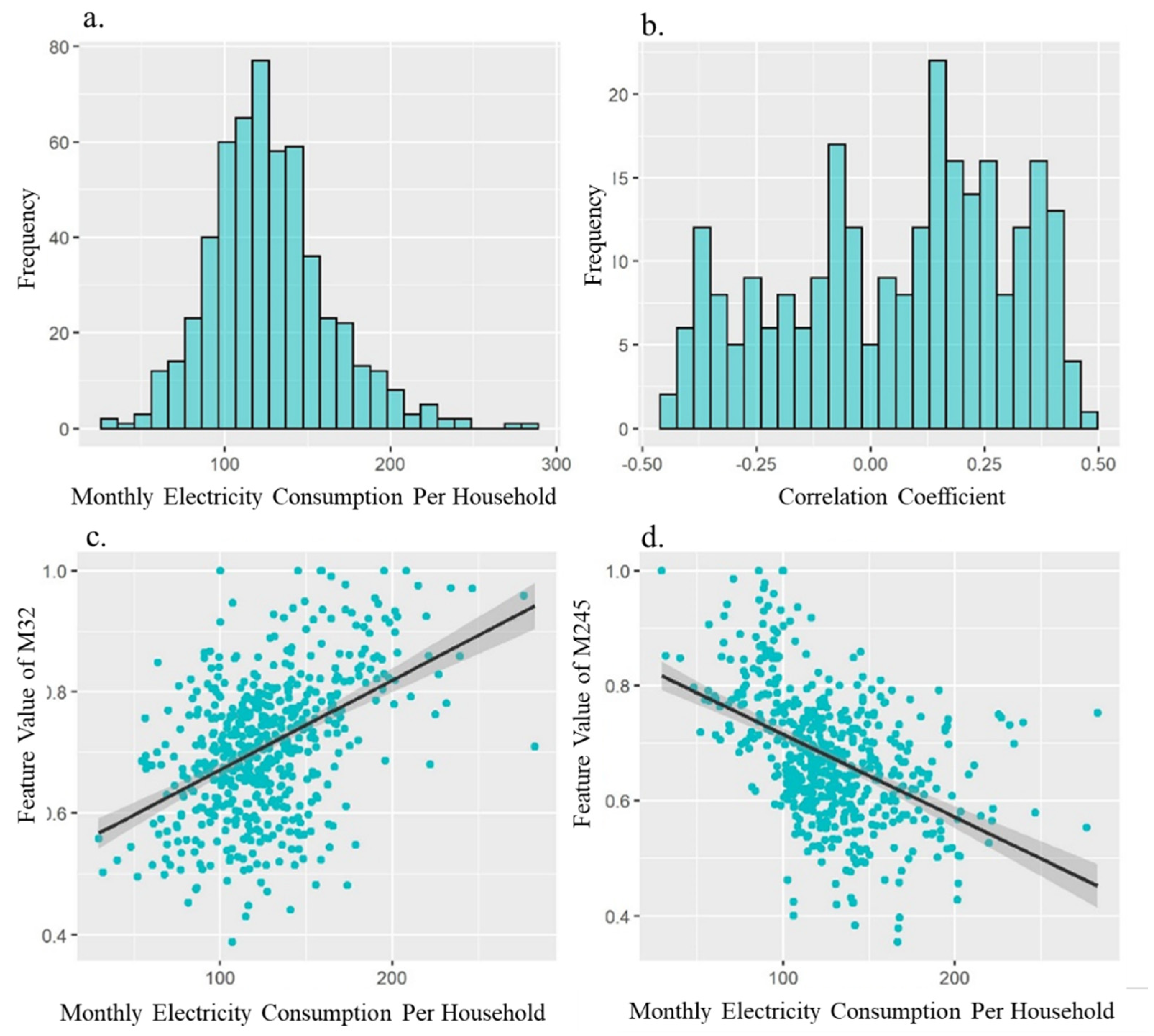
The average monthly electricity consumption of the 547 villages varied significantly. The overall electricity consumption shows a normal distribution, with an average value of 127 kWh, a maximum value of 283, a minimum value of 29, and a variance of 1307. This indicates that there is considerable variation in living standards across different villages. The question arises of whether larger variances in electricity consumption correspond to variations in certain aspects of the feature map values.
Using the average value of positively activated pixels as the feature value of the map, the Pearson correlation coefficient between the feature values and electricity consumption is calculated (Figure 4). The results show an average absolute value of the correlation coefficient of 0.22, indicating significant correlations among the 256-dimensional features extracted by the building remote sensing interpretation model and electricity consumption. The average value of the positive correlation coefficients is 0.23, with a maximum of 0.46, while the average value of the negative correlation coefficients is −0.2, with a minimum of −0.46. There are 188 significant correlation coefficients, accounting for 73%, and 80 with an absolute value greater than 0.3, accounting for 31%.

Figure 4.
Statistical analysis of a village’s electricity consumption: (a) normal distribution of the village’s monthly electricity consumption per household; (b) frequency of the correlation coefficient between electricity consumption and feature value; (c,d) two examples, M32 and M245, which display the correlation.
Based on these findings, this study further asked whether a small number of key feature map combinations can predict village electricity consumption levels, making the feature maps highly interpretable, i.e., positively activated areas are identifiable.
3.2. Assessment of Key Feature Importance
This study used a random forest model to predict the average monthly electricity consumption per household in the villages. The 256-dimensional feature map of the P2 layer was used as the feature vector input after global average pooling, while the corresponding village average electricity consumption was used as the label input. The model parameters were trained using ten-fold cross-validation. The results show that the model achieved a high correlation coefficient of 0.77, with an MAE of 13.9 and an RMSE of 25.5. Therefore, the feature maps extracted from the feature pyramids can effectively predict electricity consumption variations in the corresponding areas.
To filter the key feature maps, this study further used the SHAP model to evaluate the collinearity of each dimension’s features (Figure 5). The top 20 feature maps by contribution value are shown in the Figure 5. The 122nd feature map contributed the most to the prediction results, with higher feature values corresponding to lower electricity consumption. The 80th, 30th, 32nd, and 165th feature maps had higher feature values corresponding to higher electricity consumption.
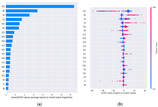
Figure 5.
The top 20 correlative feature maps inferred by the SHAP model: (a) Overall importance (absolute values) of each feature map, (b) Importance of each feature map for each sample.
If the top 10 features were used to retrain the model, the correlation coefficient (r) reached 0.780. If the top five features were used, the correlation coefficient (r) remained 0.778; if the top three features were used, the correlation coefficient (r) dropped to 0.724 (Table 1). Therefore, the top five feature maps can be considered essential inputs for predicting village electricity consumption.

Table 1.
Prediction accuracy using different dimensions of features.
3.3. Feature Interpretability Analysis and Relationship with Electricity Consumption
This section aims to explain the meanings of the geographic elements contained in each feature through feature visualization and analyze their underlying relationships from the perspective of rural geography. The previous text uses the SHAP model to obtain the five feature maps with the highest contributions. Through feature visualization, according to their primary positions of positive activation, these five feature maps can be defined as follows: all houses (M156), new houses (M30), roads and alleys (M80), farmland and forests (M122), and others (M32). The five major feature maps are significantly correlated with average household electricity consumption in villages, with farmland and forest features negatively correlated with electricity consumption, and the others positively correlated (Table 2).
Table 2.
Feature categories corresponding to feature maps and their correlation coefficients with electricity consumption.
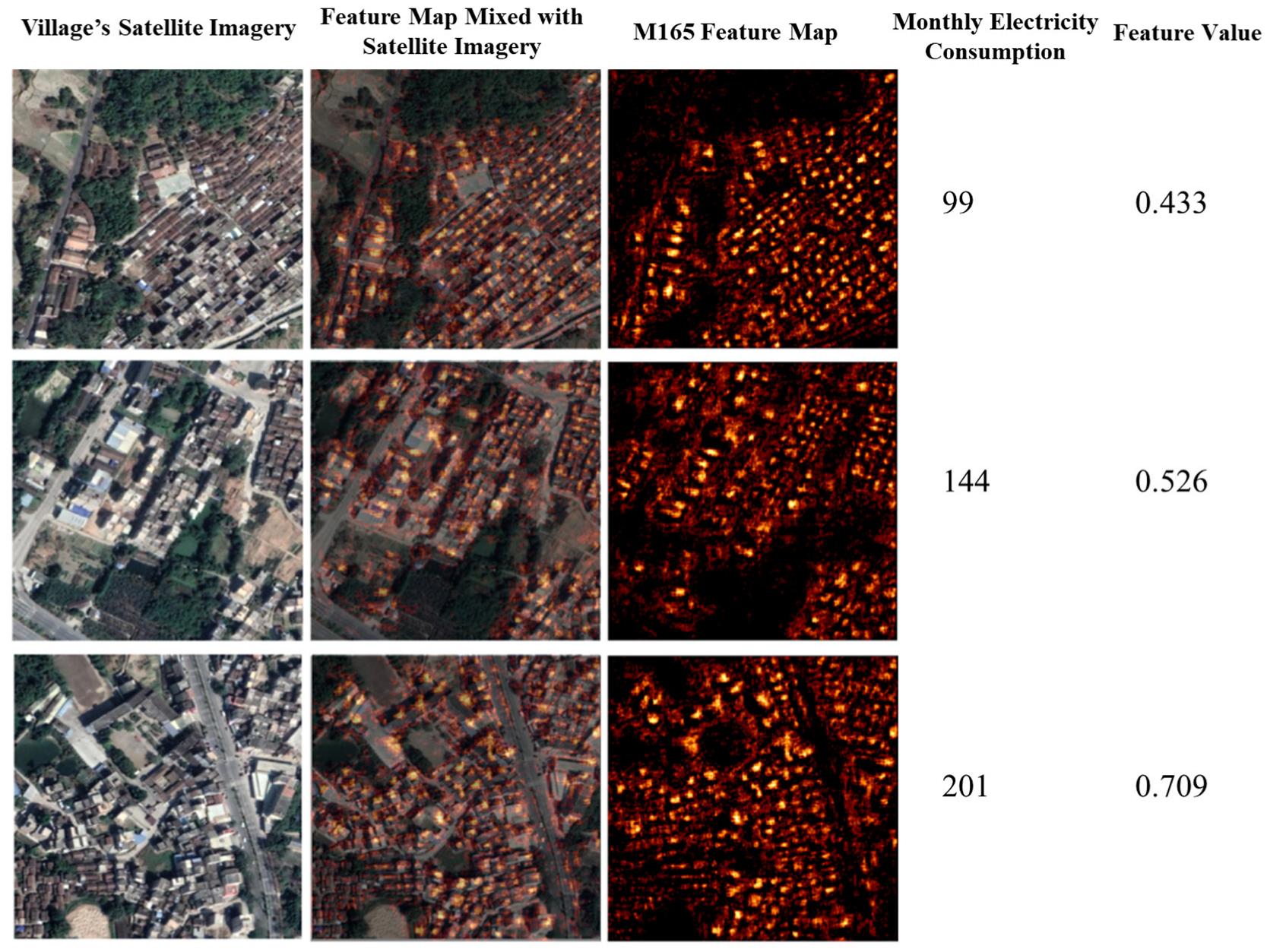
Firstly, housing features are important variables related to electricity consumption. M165 and M30 primarily activate building areas. As shown in the Figure 6, almost all building rooftops are highlighted, indicating that these areas are the most interesting to the feature map. From the perspective of positive activation, these areas contribute significantly to recognizing farmhouses at these locations. Thus, the feature pyramid successfully captures the farmhouse features at these locations. Through global average pooling, the feature map obtains the overall farmhouse features. Different images have different overall farmhouse features, corresponding to varying electricity consumption levels.
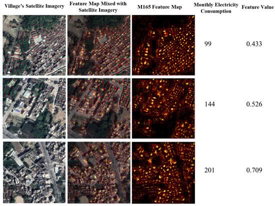
Figure 6.
Feature map M165 reflects house information (activated areas primarily correspond to building rooftops).
Housing is an important spatial carrier for household electricity consumption. Most daily activities of rural residents occur inside houses, with household electrical appliances mainly attached to houses. Appliances such as air conditioners, refrigerators, televisions, washing machines, and computers inside houses need to be connected to the power supply to function normally. Therefore, the presence of houses is the basis for the presence of electricity consumption in the area. The level of electricity consumption may be reflected in housing features. For example, larger and newer houses may have more electrical appliances and, thus, higher electricity consumption.
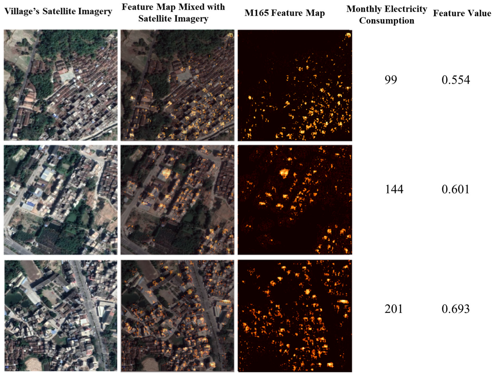
The core activation of the M30 feature map is the location of new houses, further illustrating the correlation between housing features and electricity consumption (Figure 7). As shown in the figure, the original remote sensing image of the village shows both new and old houses. Old houses have gray roofs, smaller sizes, lower floors, and are clustered together. New buildings have white or light-colored roofs, larger sizes, more building floors, and are close to major external roads. The activated parts of the feature map are mainly on the rooftops of new buildings, indicating that this feature map primarily extracts new house features. Newer houses often have more modern and efficient electrical appliances, typically with better energy efficiency and lower electricity consumption. In contrast, older houses may use older appliances with lower energy efficiency and higher electricity consumption. Therefore, the age of a house is an important supplement in predicting household electricity consumption.
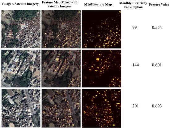
Figure 7.
Feature map M30 reflects new house information (activated areas primarily correspond to rooftops of newly constructed buildings, with newer buildings showing brighter activations, while older buildings exhibit weaker activations).
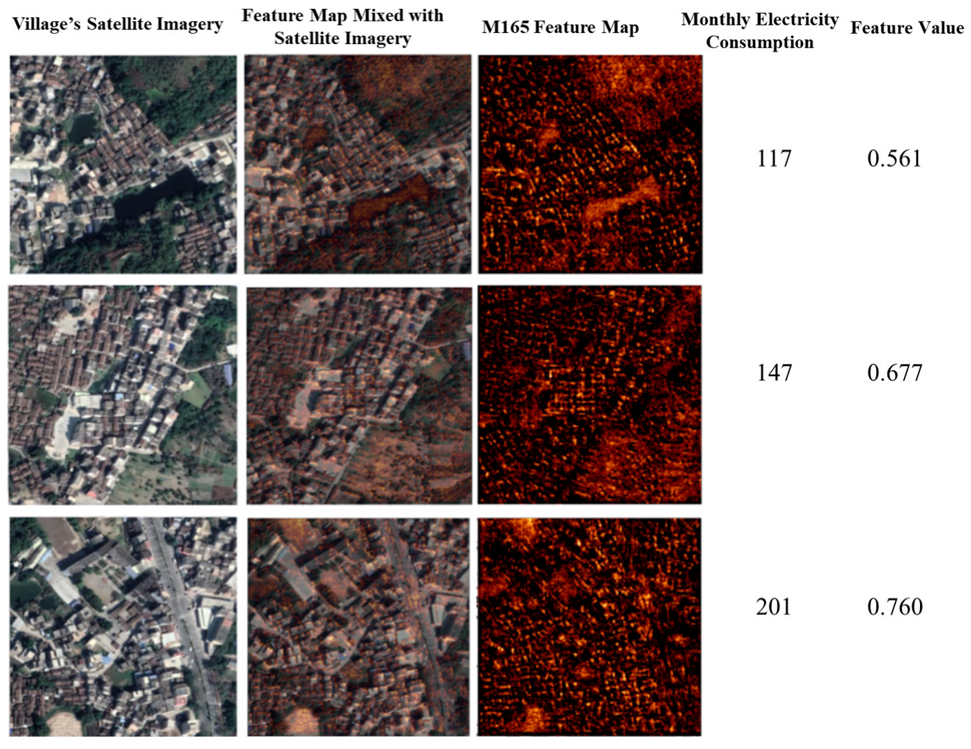
Road features are another important variable influencing village electricity consumption. Village roads are essential for daily production and life in villages. “To get rich, build roads first.” Roads promote the flow of rural elements and optimize resource allocation, bringing wealth to an area. Therefore, road construction features are closely related to electricity consumption levels. As shown in the Figure 8, the activation degree of feature maps at the spatial positions of external roads in villages is particularly noticeable. Especially for villages near industrial areas, the primary activation is for asphalt on urban main roads.
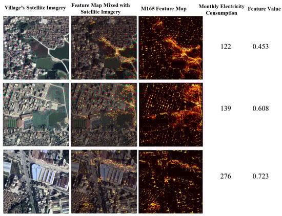
Figure 8.
Feature map M80 reflects road information (buildings closer to roads are more likely to be activated).
Farmland and forest features have a negative relationship with village electricity consumption. As shown in the Figure 9, the feature map mainly activates large green areas of forests and farmlands. The green of forests is more prominent than that of farmlands, with higher activation brightness. Therefore, this study speculates that the information extracted by this feature map is related to mountainous areas. Xinxing County is a mountainous agricultural county, with the terrain mainly consisting of mountains. Thus, many of the villages are mountain villages. The average household electricity consumption of 56 kWh in the village is an important example, being far from the county town and deep in the mountains of Huangwo village, Lidong town, located in a narrow valley leading to the town area. With inconvenient transportation and severe population outflow, the living electricity consumption level is also low. Thus, the appearance of forest features significantly reduces the electricity consumption level of the area, which is the main reason why M122 is highly negatively correlated with electricity consumption.
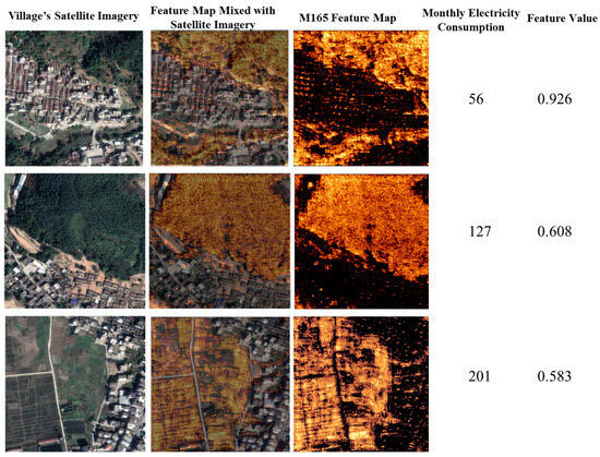
Figure 9.
Feature map M122 reflects information on forestry and farms (activated areas primarily correspond to forests and farmland).
The feature pyramid integrates deep semantic information with shallow morphological information. The activated parts of the feature map may reflect some important features of the input data, but all activated parts are not necessarily interpretable. For example, M32 has a high correlation coefficient of 0.40 with electricity consumption, but the core activated areas are unknown from the feature map. Buildings, farmland, forests, and open spaces are all activated (Figure 10), indicating that M32 is somewhat sensitive to these different types of areas. Therefore, this study cannot determine its main features, classifying it as other or composite features, indicating that it contributes to electricity consumption prediction from multiple aspects.
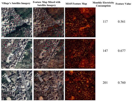
Figure 10.
Feature map M32 reflects comprehensive information (activated features cover various types, such as buildings, farmland, forests, and open spaces, representing composite characteristics).
Interpreting feature maps is a challenge in deep learning because neural network decision processes are highly complex and nonlinear. Although this study could analyze the relationship between activated parts and input data, understanding the exact meaning of specific features may require more research and experimentation.
3.4. Hyperparameter Sensitivity Analysis
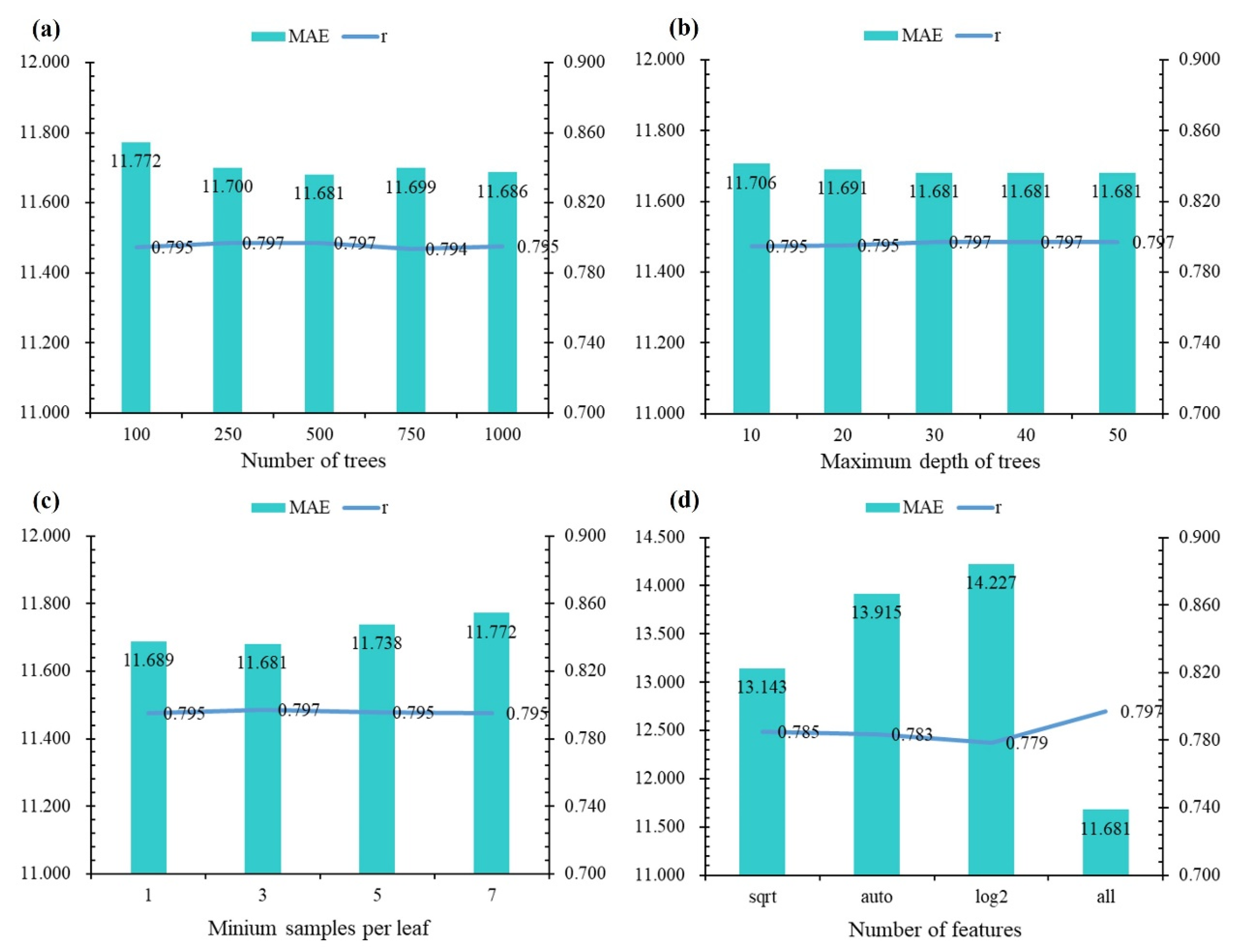
The hyperparameters, including number of trees, number of features, minimum samples per leaf, and maximum depth of trees, were optimized in the random forest algorithm. We utilized the grid search algorithm to determine the accuracy of all combinations of the hyperparameters using the correlation coefficient, r, and the MAE as the evaluation metrics. When r reaches the maximum while MAE reaches the minimum, the optimal hyperparameters were obtained. In this study, the number of trees, maximum depth of trees, minimum samples per leaf, and number of features were set to 500, 50, 3, and all, respectively (Figure 11).
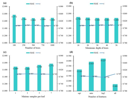
Figure 11.
Hyperparameter sensitivity analysis for Random Forest. (a) Number of trees. (b) Maximum depth of trees. (c) Minium samples per leaf. (d) Number of features.
4. Discussion
4.1. Effectiveness of the Proposed Method
Previous studies have focused solely on the direct prediction of electricity consumption from images, neglecting which information in the images contributes to the results and their underlying human geographic significance. To address this, this study proposes an interpretable electricity prediction framework that combines deep convolutional features, feature visualization, and multivariate linear regression models to predict average electricity consumption levels in villages. The study first used the Mask R-CNN network pretrained on large-scale village images to obtain features that represent village information. Subsequently, the random forest algorithm was used to regress these features against electricity consumption data. The experimental results show a correlation of 0.797 between the 256-dimensional features and electricity consumption, indicating that the extracted feature maps, indeed, contain information that can explain differences in electricity usage. To further analyze the impact of these features on electricity prediction, the SHAP model was used to interpret the feature importance. We found that using only the top 10 most important features can result in a similar accuracy as that using all 256 features. This suggests significant information redundancy in the 256-dimensional features, highlighting the necessity of feature selection. The study also evaluated the performance of the top three and top five features in predicting electricity consumption and found that the top five features provided the most explanatory power.
To further explain the human geographic implications of features predicting electricity consumption, this study visualized the feature maps and assigned geographical connotations based on expert knowledge. The experimental results show that the top five features include information reflecting dimensions such as new and old houses, roads, farmland, and forests, providing a theoretical basis for electricity consumption prediction. Furthermore, the study explored the relationship between these geographical features and electricity consumption, using the average value of positively activated pixels in feature maps as feature values to highlight important objects in each feature map. The experiment revealed that new and old houses and roads have a significant positive correlations with electricity consumption, indicating that human activities and behaviors, indeed, determine electricity usage. Farmland and forests show a significant negative correlation with electricity consumption, suggesting that production, living, and ecological spaces in these villages are separate. It also demonstrates that using the top five features for electricity consumption prediction is reasonable and feasible.
4.2. Limitations of Methods and Applications
It is important to consider the potential biases in the electricity consumption dataset. Because of the scarcity of real power consumption data and user privacy protection, this study utilized the aggregated power consumption records in the study area, Xinxing County. Two types of biases are potentially introduced into the model. The first type of bias is regional sample bias, related to geographic heterogeneity, which follows the universal pattern described by the second law of geography. It refers to the impact of geographical differences due to natural, economic, social, and other factors that may introduce regional bias. The universal pattern represents the challenge that GeoAI is seeking to address. The second type of bias is the random disturbances added to protect user privacy. To mitigate these potential biases, we employed 10-fold cross-validation and randomly dropping branches of random forests. We believe these commonly used techniques reduce the risk of overfitting to our dataset.
In terms of methodology, although pretrained image features have high correlations with electricity consumption, especially the top 5 features that can be interpreted geographically, the results show that the top 10 features have even higher correlations with electricity consumption. The reason for not using the top 10 features to predict electricity consumption is that some feature visualization maps are difficult to explain through expert knowledge. These features may represent nonlinear abstract information, such as settlement morphology, spatial layout of elements, and element proportion combinations, rather than single-element representations. Therefore, the interpretability of features needs further research, especially in explaining macro-level abstract information. Additionally, the SHAP model requires improvements to better capture complex geographical relationships. It is precisely because SHAP does not have enough understanding of complex features that the extracted key features have certain deviations, which affects the final results. Secondly, since the feature maps are converted into feature values by averaging the positively activated pixels, the information on the original features is compressed to a certain extent, which also affects the final prediction result.
Similarly, because of the current immaturity of machine learning interpretability, some limitations have been imposed on our research. Because of the difficulty in obtaining electricity data, this study focused on one county, which may represent only one type of village pattern and could differ from others. However, the main purposes of this study were to determine whether electricity consumption can be predicted from remote sensing images and to explain the geographical features that influence electricity prediction. In different regions, these features and regression coefficients may vary, but the prediction and explanation patterns remain essentially the same. Therefore, the framework and approach proposed in this paper can be applied to study different rural settlements and are equally applicable to large-scale regional predictions, potentially revealing spatial heterogeneity in village electricity consumption and geographical features.
5. Conclusions
This study proposes a straightforward XAI framework that combines deep convolutional features, feature visualization, and multiple linear regression models to predict average electricity consumption levels in villages. The study identifies key deep convolutional features affecting average electricity consumption levels, including new/old farmhouses, external roads, farmland, forests, and public spaces. These features reflect the socio-economic vitality of villages, answering why deep convolutional features can predict average electricity levels, providing a method for national- and global-level electricity mapping in response to SDG 7.
Currently, there is no suitable XAI in the SIML field that can effectively explain the relationship between deep convolutional features and the topics of interest. This study proposes an effective XAI framework that constructs an explanatory model between deep convolutional features and average electricity levels using a simple multiple linear model. The model shows strong prediction results in both training and testing sets, indicating its generalizability for predicting average electricity levels. Additionally, the model combines feature visualization to analyze to which geographic elements the key deep convolutional features correspond. This interpretability increases the reliability of the method. Instead of relying on abstract numerical features that may be difficult to relate to real-world scenarios, the study uses feature maps corresponding to tangible environmental elements. This approach provides both predictions and explanations of which specific geographic elements contribute to electricity consumption patterns.
This framework has the limitation of not considering the impact of electricity-fee reduction policies for low-income households. In regions with poverty assistance, households benefiting from electricity-fee reduction policies may appropriately increase their electricity consumption to improve their living standards. However, upgrading geographic elements, such as houses, roads, and farmland, remains challenging. This means there may be situations in which the average electricity level implied by the village’s geographic elements do not fully match the actual electricity consumption. Although this situation is usually rare, linear models cannot simulate this, leading to some errors in the results. Future research will consider using nonlinear regression models to construct more advanced explanatory models to address this issue.
Author Contributions
Conceptualization, Yaofu Huang and Xun Li; Funding acquisition, Xun Li; Investigation, Weipan Xu and Dongsheng Chen; Methodology, Yaofu Huang and Weipan Xu; Software, Weipan Xu and Dongsheng Chen; Validation, Weihuan Deng and Xun Li; Visualization, Yaofu Huang and Dongsheng Chen; Writing—original draft, Yaofu Huang; Writing—review and editing, Yaofu Huang, Qiumeng Li and Xun Li. All authors have read and agreed to the published version of the manuscript.
Funding
This research was funded by the National Natural Science Foundation of China, grant number: 42371206.
Data Availability Statement
The data presented in this study are available only upon request from the corresponding author because the village electricity data contain sensitive information.
Conflicts of Interest
The authors declare no conflicts of interest.
References
- United Nations. Transforming Our World: The 2030 Agenda for Sustainable Development; United Nations Department of Economic and Social Affairs: New York, NY, USA, 2015. [Google Scholar]
- He, J.; Yang, Y.; Liao, Z.; Xu, A.; Fang, K. Linking SDG 7 to Assess the Renewable Energy Footprint of Nations by 2030. Appl. Energy 2022, 317, 119167. [Google Scholar] [CrossRef]
- Parra, C.; Kirschke, J.; Ali, S.H. Ensure Access to Affordable, Reliable, Sustainable and Modern Energy for All. In Mining, Materials, and the Sustainable Development Goals (SDGs); CRC Press: Boca Raton, FL, USA, 2020; pp. 61–68. [Google Scholar]
- International Energy Agency. Global Energy Review 2020; International Energy Agency: Paris, France, 2020. [Google Scholar]
- Trinh, V.L.; Chung, C.K. Renewable Energy for SDG-7 and Sustainable Electrical Production, Integration, Industrial Application, and Globalization. Clean. Eng. Technol. 2023, 15, 100657. [Google Scholar] [CrossRef]
- Jean, N.; Burke, M.; Xie, M.; Davis, W.M.; Lobell, D.B.; Ermon, S. Combining Satellite Imagery and Machine Learning to Predict Poverty. Science 2016, 353, 790–794. [Google Scholar] [CrossRef] [PubMed]
- Yeh, C.; Perez, A.; Driscoll, A.; Azzari, G.; Tang, Z.; Lobell, D.; Ermon, S.; Burke, M. Using Publicly Available Satellite Imagery and Deep Learning to Understand Economic Well-Being in Africa. Nat. Commun. 2020, 11, 2583. [Google Scholar] [CrossRef] [PubMed]
- Rolf, E.; Proctor, J.; Carleton, T.; Bolliger, I.; Shankar, V.; Ishihara, M.; Recht, B.; Hsiang, S. A Generalizable and Accessible Approach to Machine Learning with Global Satellite Imagery. Nat. Commun. 2021, 12, 4392. [Google Scholar] [CrossRef]
- Burke, M.; Driscoll, A.; Lobell, D.B.; Ermon, S. Using Satellite Imagery to Understand and Promote Sustainable Development. Science 2021, 371, eabe8628. [Google Scholar] [CrossRef]
- Mosavi, A.; Salimi, M.; Faizollahzadeh Ardabili, S.; Rabczuk, T.; Shamshirband, S.; Varkonyi-Koczy, A.R. State of the Art of Machine Learning Models in Energy Systems, a Systematic Review. Energies 2019, 12, 1301. [Google Scholar] [CrossRef]
- Hong, T.; Wang, Z.; Luo, X.; Zhang, W. State-of-the-Art on Research and Applications of Machine Learning in the Building Life Cycle. Energy Build. 2020, 212, 109831. [Google Scholar] [CrossRef]
- Fathi, S.; Srinivasan, R.; Fenner, A.; Fathi, S. Machine Learning Applications in Urban Building Energy Performance Forecasting: A Systematic Review. Renew. Sustain. Energy Rev. 2020, 133, 110287. [Google Scholar] [CrossRef]
- Amasyali, K.; El-Gohary, N.M. A Review of Data-Driven Building Energy Consumption Prediction Studies. Renew. Sustain. Energy Rev. 2018, 81, 1192–1205. [Google Scholar] [CrossRef]
- Ahmad, T.; Chen, H.; Guo, Y.; Wang, J. A Comprehensive Overview on the Data Driven and Large Scale Based Approaches for Forecasting of Building Energy Demand: A Review. Energy Build. 2018, 165, 301–320. [Google Scholar] [CrossRef]
- Mahmood, S.; Sun, H.; Alhussan, A.A.; Iqbal, A.; El-Kenawy, E.S.M. Active Learning-Based Machine Learning Approach for Enhancing Environmental Sustainability in Green Building Energy Consumption. Sci. Rep. 2024, 14, 19894. [Google Scholar] [CrossRef] [PubMed]
- Bhattarai, D.; Lucieer, A.; Lovell, H.; Aryal, J. Remote Sensing of Night-time Lights and Electricity Consumption: A Systematic Literature Review and Meta-analysis. Geogr. Compass 2023, 17, e12684. [Google Scholar] [CrossRef]
- Jang, H.S.; Bae, K.Y.; Park, H.-S.; Sung, D.K. Solar Power Prediction Based on Satellite Images and Support Vector Machine. IEEE Trans. Sustain. Energy 2016, 7, 1255–1263. [Google Scholar] [CrossRef]
- Ferreira, B.; Silva, R.G.; Iten, M. Earth Observation Satellite Imagery Information Based Decision Support Using Machine Learning. Remote Sens. 2022, 14, 3776. [Google Scholar] [CrossRef]
- Doll, C.N.; Pachauri, S. Estimating Rural Populations without Access to Electricity in Developing Countries through Night-Time Light Satellite Imagery. Energy Policy 2010, 38, 5661–5670. [Google Scholar] [CrossRef]
- Townsend, A.C.; Bruce, D.A. The Use of Night-Time Lights Satellite Imagery as a Measure of Australia’s Regional Electricity Consumption and Population Distribution. Int. J. Remote Sens. 2010, 31, 4459–4480. [Google Scholar] [CrossRef]
- Elvidge, C.D.; Hsu, F.-C.; Zhizhin, M.; Ghosh, T.; Taneja, J.; Bazilian, M. Indicators of Electric Power Instability from Satellite Observed Nighttime Lights. Remote Sens. 2020, 12, 3194. [Google Scholar] [CrossRef]
- Sun, Y.; Wang, S.; Zhang, X.; Chan, T.O.; Wu, W. Estimating Local-Scale Domestic Electricity Energy Consumption Using Demographic, Nighttime Light Imagery and Twitter Data. Energy 2021, 226, 120351. [Google Scholar] [CrossRef]
- Elvidge, C.D.; Baugh, K.E.; Kihn, E.A.; Kroehl, H.W.; Davis, E.R.; Davis, C.W. Relation between Satellite Observed Visible-near Infrared Emissions, Population, Economic Activity and Electric Power Consumption. Int. J. Remote Sens. 1997, 18, 1373–1379. [Google Scholar] [CrossRef]
- Lin, J.; Shi, W. Statistical Correlation between Monthly Electric Power Consumption and VIIRS Nighttime Light. ISPRS Int. J. Geo-Inf. 2020, 9, 32. [Google Scholar] [CrossRef]
- Chen, J.; Gao, M.; Cheng, S.; Hou, W.; Song, M.; Liu, X.; Liu, Y. Global 1 Km\times 1 Km Gridded Revised Real Gross Domestic Product and Electricity Consumption during 1992–2019 Based on Calibrated Nighttime Light Data. Sci. Data 2022, 9, 202. [Google Scholar] [CrossRef] [PubMed]
- Zhao, M.; Zhou, Y.; Li, X.; Cao, W.; He, C.; Yu, B.; Li, X.; Elvidge, C.D.; Cheng, W.; Zhou, C. Applications of Satellite Remote Sensing of Nighttime Light Observations: Advances, Challenges, and Perspectives. Remote Sens. 2019, 11, 1971. [Google Scholar] [CrossRef]
- Zheng, Q.; Seto, K.C.; Zhou, Y.; You, S.; Weng, Q. Nighttime Light Remote Sensing for Urban Applications: Progress, Challenges, and Prospects. ISPRS J. Photogramm. Remote Sens. 2023, 202, 125–141. [Google Scholar] [CrossRef]
- Levin, N.; Kyba, C.C.; Zhang, Q.; de Miguel, A.S.; Román, M.O.; Li, X.; Portnov, B.A.; Molthan, A.L.; Jechow, A.; Miller, S.D. Remote Sensing of Night Lights: A Review and an Outlook for the Future. Remote Sens. Environ. 2020, 237, 111443. [Google Scholar] [CrossRef]
- Chu, L.; Oloo, F.; Sudmanns, M.; Tiede, D.; Hölbling, D.; Blaschke, T.; Teleoaca, I. Monitoring Long-Term Shoreline Dynamics and Human Activities in the Hangzhou Bay, China, Combining Daytime and Nighttime EO Data. Big Earth Data 2020, 4, 242–264. [Google Scholar] [CrossRef]
- Xing, X.; Huang, Z.; Cheng, X.; Zhu, D.; Kang, C.; Zhang, F.; Liu, Y. Mapping Human Activity Volumes through Remote Sensing Imagery. IEEE J. Sel. Top. Appl. Earth Obs. Remote Sens. 2020, 13, 5652–5668. [Google Scholar] [CrossRef]
- Streltsov, A.; Malof, J.M.; Huang, B.; Bradbury, K. Estimating Residential Building Energy Consumption Using Overhead Imagery. Appl. Energy 2020, 280, 116018. [Google Scholar] [CrossRef]
- Wang, J.; Lu, F. Modeling the Electricity Consumption by Combining Land Use Types and Landscape Patterns with Nighttime Light Imagery. Energy 2021, 234, 121305. [Google Scholar] [CrossRef]
- Hsu, C.-Y.; Li, W. Explainable GeoAI: Can Saliency Maps Help Interpret Artificial Intelligence’s Learning Process? An Empirical Study on Natural Feature Detection. Int. J. Geogr. Inf. Sci. 2023, 37, 963–987. [Google Scholar] [CrossRef]
- Arrieta, A.B.; Díaz-Rodríguez, N.; Del Ser, J.; Bennetot, A.; Tabik, S.; Barbado, A.; García, S.; Gil-López, S.; Molina, D.; Benjamins, R. Explainable Artificial Intelligence (XAI): Concepts, Taxonomies, Opportunities and Challenges toward Responsible AI. Inf. Fusion 2020, 58, 82–115. [Google Scholar] [CrossRef]
- Thakur, R.; Rane, D. Machine Learning and Deep Learning for Intelligent and Smart Applications. In Future Trends in 5G and 6G; CRC Press: Boca Raton, FL, USA, 2021; pp. 95–113. [Google Scholar]
- Roussel, C.; Böhm, K. Geospatial Xai: A Review. ISPRS Int. J. Geo-Inf. 2023, 12, 355. [Google Scholar] [CrossRef]
- Wenninger, S.; Karnebogen, P.; Lehmann, S.; Menzinger, T.; Reckstadt, M. Evidence for Residential Building Retrofitting Practices Using Explainable AI and Socio-Demographic Data. Energy Rep. 2022, 8, 13514–13528. [Google Scholar] [CrossRef]
- Shafique, A.; Cao, G.; Khan, Z.; Asad, M.; Aslam, M. Deep Learning-Based Change Detection in Remote Sensing Images: A Review. Remote Sens. 2022, 14, 871. [Google Scholar] [CrossRef]
- Bengio, Y.; Courville, A.; Vincent, P. Representation Learning: A Review and New Perspectives. IEEE Trans. Pattern Anal. Mach. Intell. 2013, 35, 1798–1828. [Google Scholar] [CrossRef] [PubMed]
- Ma, Y.; Wu, H.; Wang, L.; Huang, B.; Ranjan, R.; Zomaya, A.; Jie, W. Remote Sensing Big Data Computing: Challenges and Opportunities. Future Gener. Comput. Syst. 2015, 51, 47–60. [Google Scholar] [CrossRef]
- González Garibay, M.; Primc, K.; Slabe-Erker, R. Insights into Advanced Models for Energy Poverty Forecasting. Nat. Energy 2023, 8, 903–905. [Google Scholar] [CrossRef]
- Li, Y.; Xu, W.; Chen, H.; Jiang, J.; Li, X. A Novel Framework Based on Mask R-CNN and Histogram Thresholding for Scalable Segmentation of New and Old Rural Buildings. Remote Sens. 2021, 13, 1070. [Google Scholar] [CrossRef]
- Xu, W.; Gu, Y.; Chen, Y.; Wang, Y.; Chen, L.; Deng, W.; Li, X. Combining Deep Learning and Crowd-Sourcing Images to Predict Housing Quality in Rural China. Sci. Rep. 2022, 12, 19558. [Google Scholar] [CrossRef]
- Deng, W.; Xu, W.; Huang, Y.; Li, X. A Large-Scale Multipurpose Benchmark Dataset and Real-Time Interpretation Platform Based on Chinese Rural Buildings. IEEE J. Sel. Top. Appl. Earth Obs. Remote Sens. 2024, 17, 10914–10928. [Google Scholar] [CrossRef]
- Li, Z. Extracting Spatial Effects from Machine Learning Model Using Local Interpretation Method: An Example of SHAP and XGBoost. Comput. Environ. Urban Syst. 2022, 96, 101845. [Google Scholar] [CrossRef]
- He, K.; Gkioxari, G.; Dollár, P.; Girshick, R. Mask R-Cnn. In Proceedings of the IEEE International Conference on Computer Vision, Venice, Italy, 22–29 October 2017; pp. 2961–2969. [Google Scholar]
- Ran, S.; Gao, X.; Yang, Y.; Li, S.; Zhang, G.; Wang, P. Building Multi-Feature Fusion Refined Network for Building Extraction from High-Resolution Remote Sensing Images. Remote Sens. 2021, 13, 2794. [Google Scholar] [CrossRef]
- Lu, T.; Ming, D.; Lin, X.; Hong, Z.; Bai, X.; Fang, J. Detecting Building Edges from High Spatial Resolution Remote Sensing Imagery Using Richer Convolution Features Network. Remote Sens. 2018, 10, 1496. [Google Scholar] [CrossRef]
- Guo, H.; Du, B.; Zhang, L.; Su, X. A Coarse-to-Fine Boundary Refinement Network for Building Footprint Extraction from Remote Sensing Imagery. ISPRS J. Photogramm. Remote Sens. 2022, 183, 240–252. [Google Scholar] [CrossRef]
- Zhu, Q.; Li, Z.; Zhang, Y.; Guan, Q. Building Extraction from High Spatial Resolution Remote Sensing Images via Multiscale-Aware and Segmentation-Prior Conditional Random Fields. Remote Sens. 2020, 12, 3983. [Google Scholar] [CrossRef]
- Chen, S.; Zhang, Y.; Nie, K.; Li, X.; Wang, W. Extracting Building Areas from Photogrammetric DSM and DOM by Automatically Selecting Training Samples from Historical DLG Data. ISPRS Int. J. Geo-Inf. 2020, 9, 18. [Google Scholar] [CrossRef]
- Huang, H.; Chen, Y.; Wang, R. A Lightweight Network for Building Extraction from Remote Sensing Images. IEEE Trans. Geosci. Remote Sens. 2021, 60, 5614812. [Google Scholar] [CrossRef]


Disclaimer/Publisher’s Note: The statements, opinions and data contained in all publications are solely those of the individual author(s) and contributor(s) and not of MDPI and/or the editor(s). MDPI and/or the editor(s) disclaim responsibility for any injury to people or property resulting from any ideas, methods, instructions or products referred to in the content. |
© 2024 by the authors. Published by MDPI on behalf of the International Society for Photogrammetry and Remote Sensing. Licensee MDPI, Basel, Switzerland. This article is an open access article distributed under the terms and conditions of the Creative Commons Attribution (CC BY) license (https://creativecommons.org/licenses/by/4.0/).