Article

Spatial Correlation between the Changes in Supply and Demand for Water-Related Ecosystem Services

School of Environment and Spatial Informatics, China University of Mining and Technology, Xuzhou 221116, China
*
Author to whom correspondence should be addressed.
ISPRS Int. J. Geo-Inf. 2024, 13(3), 68; https://doi.org/10.3390/ijgi13030068
Submission received: 8 January 2024 / Revised: 15 February 2024 / Accepted: 21 February 2024 / Published: 23 February 2024

Abstract

:
Clarifying the spatiotemporal changes in the supply and demand of water-related ecosystem services (WESs) can provide comprehensive support information for ecological governance decisions. However, the spatial mismatch between the supply and demand of WESs is often overlooked, resulting in a lack of targeted decision-making. At the grid scale, while preserving both natural and social attributes, this study quantitatively analyzed the spatiotemporal changes in the supply and demand of WESs in the Southern River Basin from 2000 to 2020. Ecological zoning was performed based on the temporal changes in WESs supply and demand. The OPGD model was used to investigate the impacts of socio-economic and natural factors on different WESs supply factors and further explore the spatial correlation of WESs supply and demand changes in different zones. The results show that there is significant spatial heterogeneity in the changes in WESs supply and demand. Economic belts and megacities have experienced remarkable changes, with WESs supply decreasing and WESs demand increasing. WESs demand changes significantly affect WESs supply changes. The supply of WESs in all zones is influenced by WESs demand. In the high supply–low demand zone, WY has the highest explanatory power for WESs demand changes. From the high supply–middle demand zone to the low supply–middle demand zone and then to the high supply–high demand zone, the explanatory power of PE for WESs demand changes gradually increases. As WESs demand starts from the middle level, HAI gradually dominates WESs demand changes. The increase in land use changes may promote the impact of WESs demand changes on WESs supply changes. This study contributes to incorporating the supply and demand changes of WESs and their correlations into the ecological protection and restoration system, providing a new perspective and method for regional sustainable management.

1. Introduction

Ecosystem services (ESs) refer to the direct or indirect benefits that humans obtain from ecosystems [1,2], constituting a fundamental source of human well-being [3]. As humans have predominantly prioritized urban socio-economic development over time, the capacity of ESs to deliver essential services, which society relies upon, has gradually diminished [4,5]. The rapid increase in ecological issues like biodiversity loss, soil erosion, groundwater depletion, and degradation of water quality in these urban areas poses significant threats to the region’s sustainable development [6,7]. Consequently, the majority of ESs (nature’s contributions to humans) are experiencing a decline [8]. Over the past 50 years, approximately 60% of global ESs have degraded, seriously affecting the long-term sustainability of the ecosystem [9,10]. Should human activities persist in recklessly disrupting the structure and functionality of natural ESs, projections suggest that global economic losses from land degradation could escalate to USD 23 trillion by 2050 [11]. In this context, effectively improving ESs on a global scale has emerged as a critical issue in the fields of sustainable development and natural resource management over the past 20 years [8]. Moreover, ESs possess both natural and social attributes. Ecosystems’ structure and functions do not inherently constitute ESs without humans as beneficiaries and consumers [12]. Water-related ecosystem services (WESs) represent a distinct category of ESs originating from terrestrial ecosystems’ interaction with hydrological processes. They play a pivotal role in fulfilling human requirements and preserving ecosystem health [13,14]. WESs are encompassed within various categories of ESs. For instance, WESs encompass providing water resources for human use (supply services), influencing soil conservation and biodiversity maintenance (supporting services), contributing to water cycling and purification (regulation services), and offering natural landscapes for ecotourism along rivers and lakes (cultural services) [15,16]. Therefore, from the perspective of multiple stakeholders, the demand for WESs should be given adequate attention [17]. Given the supply and demand of WESs, a strong connection has been established between natural WESs and socio-economic systems, providing a practical approach to analyzing society’s relationship with water-related ecosystems [15]. Furthermore, an in-depth exploration of the spatial correlation between WESs supply and demand, as well as its influencing factors, can facilitate the integration of WESs into ecosystem management, ultimately minimizing losses, preserving and restoring damaged water-related ecosystems.
In the field of WESs research, there is a growing emphasis on the significance of both supply and demand aspects of WESs. Model development, participatory surveys, and spatial mapping techniques have been the dominant methodologies in this area of research [18,19,20]. The scope of these studies encompasses various grids, counties, cities, regions, and countries [21,22,23,24]. From a research perspective, there has been relatively limited attention paid to the study of the matching between supply and demand in WESs. Some studies have explored the spatial mismatch patterns of WESs supply and demand from the perspectives of various stakeholders by identifying WESs supply and demand clusters. For example, Chen et al. [25] conducted a study that quantified the balance between supply and demand of WESs in highly urbanized cities in 2016. Liang et al. [26] evaluated the response of land use and land cover (LULC) to WESs in three different periods over three years. Liu et al. [27] quantified the supply, demand, and spatial flow of WESs in 2010. Wu et al. [28] analyzed the impact of megacity urban land expansion on WESs in four different periods. However, most existing studies rely on the spatial patterns of a single year to depict the correlation between the supply and demand of WESs, which can only provide static information. The dynamic variations in the supply and demand of WESs can reveal the dynamic characteristics of the WESs supply and demand relationship. Integrating the spatial characteristics of dynamic changes in WESs supply and demand will facilitate a deeper understanding of the relationships between WESs supply and demand. The supply and demand of WESs are influenced and constrained by geographical space [29]. Given the spatial instability of natural environments and socio-economic conditions in different regions, the level of correlation between supply and demand changes in WESs may vary [30]. The application of global spatial analysis methods may, to some extent, mask the differences in information presentation across certain regions. Therefore, when analyzing the dynamic changes in the supply and demand of WESs, the spatial pattern can be comprehensively considered for zoning. Spatial units within each zone exhibit similar WESs supply and demand, which facilitates a genuine and comprehensive understanding of the correlations between WESs supply and demand variations.
The examination of ecological and socioeconomic factors that influence the spatial distribution of WESs systems is attracting growing interest. Statistical methods such as regression analysis, correlation analysis, factor analysis, cluster analysis, and multivariate analysis, have been devised to evaluate the effects of various factors, encompassing socioeconomic and natural elements, on water-related ecosystems and their services [31,32,33,34]. These methods aid in identifying crucial drivers, determining the strength of associations between variables, and offering insights into the intricate interplay among socioeconomic, natural factors, and WESs [35]. However, these techniques have their limitations. They often focus on individual factors, which makes it challenging to capture the intricate relationships among variables. Furthermore, these approaches might struggle to measure the individual contributions of influential factors or accommodate multivariate covariance, potentially resulting in an incomplete or biased comprehension of the underlying processes [36]. The Geodetector model (GDM) offers a robust approach to addressing these challenges by effectively identifying the contribution of single factors. The GDM is designed to mitigate the limitations of traditional statistical methods, enabling a more comprehensive understanding of the complex relationships between natural socio-economic and WESs supply and demand [37]. However, the traditional GDM primarily utilizes empirical knowledge for classifying spatial data, which tends to be subjective. Therefore, we introduce the optimal parameter-based geographical detector (OPGD), which selects the classification parameter combination with the highest q-value to discretize continuous variables, thereby enhancing the quantitative investigation of the driving mechanisms behind WESs supply and demand.
The Southern River Basin, located in a region with complex geographical features in China, boasts a wide variety of landforms, with mountains and hills as the dominant types. The Southern River Basin encompasses the Yangtze River Basin (YRB) and the Pearl River Basin (PRB), two major water systems in China which are closely linked to the supply and demand of WESs [38]. Since the adoption of the reform and opening-up policy, with rapid economic development, continuous population agglomeration, and accelerated urbanization, the WESs in the Southern River Basin have been continuously eroded and damaged, leading to an increasing inability of the WESs supply capabilities in some cities to meet rising ecological demands [39]. In order to address these challenges, it is crucial to conduct an in-depth investigation into the supply and demand relationships and driving factors of WESs in the Southern River Basin, thereby ensuring the sustainable utilization of WESs, ecological balance, and economic prosperity. However, even with an appropriate research object, if the analysis of the supply and demand of WESs is not conducted at an appropriate spatial scale, the difficulty of decision-making and implementation will increase. Currently, some ecological regionalization studies are based on administrative boundaries or natural attributes to divide geographic units. However, when administrative units are demarcated, the natural attributes of the region are often overlooked; similarly, when natural attributes are divided, administrative units are seldom taken into account. The segmentation between natural attributes and administrative boundaries often weakens the integrity of the characteristics of supply and demand changes in WESs within the research units. As the smallest research unit, grids possess both natural and social attributes, which can not only reflect the integrity of natural attributes but also effectively capture socio-economic characteristics. Therefore, using grids as the unit of analysis can effectively showcase the characteristics of supply and demand changes in WESs while facilitating ecological governance.
This study aims to quantitatively evaluate the spatial distribution and driving factors of WESs supply and demand changes in the Southern River Basin from 2000 to 2020 at a grid scale. By comprehensively considering the spatial characteristics of WESs supply and demand dynamic changes, ecological zoning is conducted. The OPGD method is used to explore the spatial correlation of WESs supply and demand in different zones.

2. Methodology

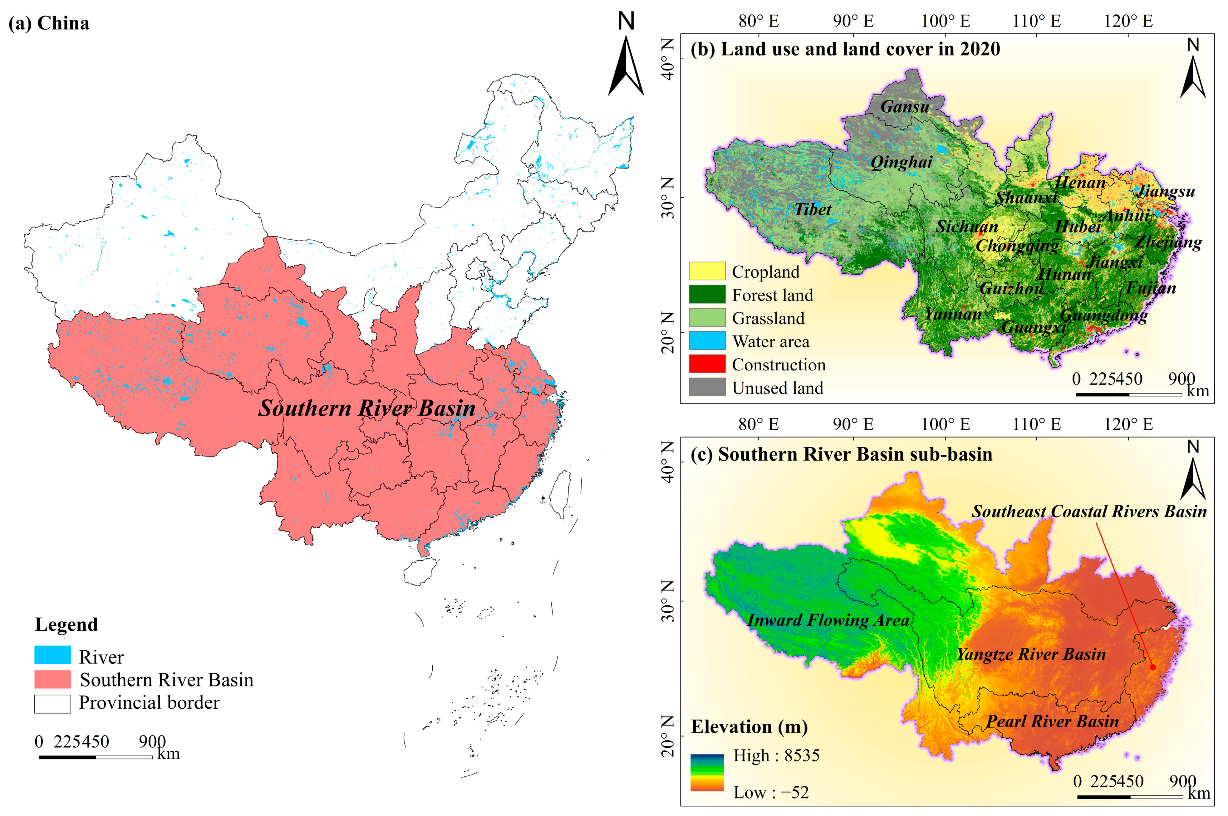
2.1. Study Site and Data Source

The Southern River Basin is situated in the southern part of China, with a geographical coordinate range of 78°25′ E to 122°12′ E east longitude and 20°09′ N to 42°48′ N north latitude (as shown in Figure 1). The Southern River Basin, encompassing the YRB and PRB, includes 19 provinces and 130 prefecture-level cities. To fully consider the integrity of social and natural attributes, this paper will conduct a simultaneous study of these 19 provinces.
The YRB is the largest river in Asia and the third longest globally. Within the YRB, three national-level city clusters exist: the Chengdu–Chongqing city cluster, the city cluster situated within the middle stretches of the Yangtze River, and the urban agglomeration of the Yangtze River Delta. In 2020, the permanent population of the YRB reached 45,697.2 million, with a gross domestic product (GDP) of CNY 35,647.48 billion, accounting for 35.2% of the national total. It is the largest basin in China in terms of drainage area, GDP, and population [40]. The yearly mean temperature distribution across the YRB reveals higher temperatures in the east and lower temperatures in the west, higher in the south and lower in the north, with the middle and lower reaches experiencing higher temperatures compared to the upper reaches. The region with exceptionally high annual precipitation exceeding 1600 mm is primarily situated in the middle and lower reaches of the river basin, whereas the semi-humid zone, with annual precipitation ranging between 400 and 800 mm, is mainly found in the upper reaches of the river basin.
The PRB comprises four primary tributaries: the Xijiang River, the Beijiang River, the Dongjiang River, and the Pearl River Delta [41]. Situated within the Pearl River Delta are numerous metropolitan areas, including Guangzhou to the north, Macau to the southwest, and Hong Kong to the southeast. In 2020, the PRB had the highest urbanization level, with a permanent population of 15,767.9 million and a GDP of CNY 122,639.4 billion, accounting for 12.10% of the national total. Its economic development level ranked second among the seven major river basins [42].
The Southern River Basin experiences a diminishing supply of ecosystem services due to ongoing encroachment of construction on cropland and natural ecosystems [14,43]. Simultaneously, accelerated urbanization intensifies the demand for WESs. This escalating disparity between supply and demand is posing an increasingly severe challenge.
In this study, various datasets were utilized. Specific information regarding the data and their respective sources can be found in Table 1.

2.2. Quantification of Water-Related Ecosystem Services

2.2.1. Water-Related Ecosystem Services Selection
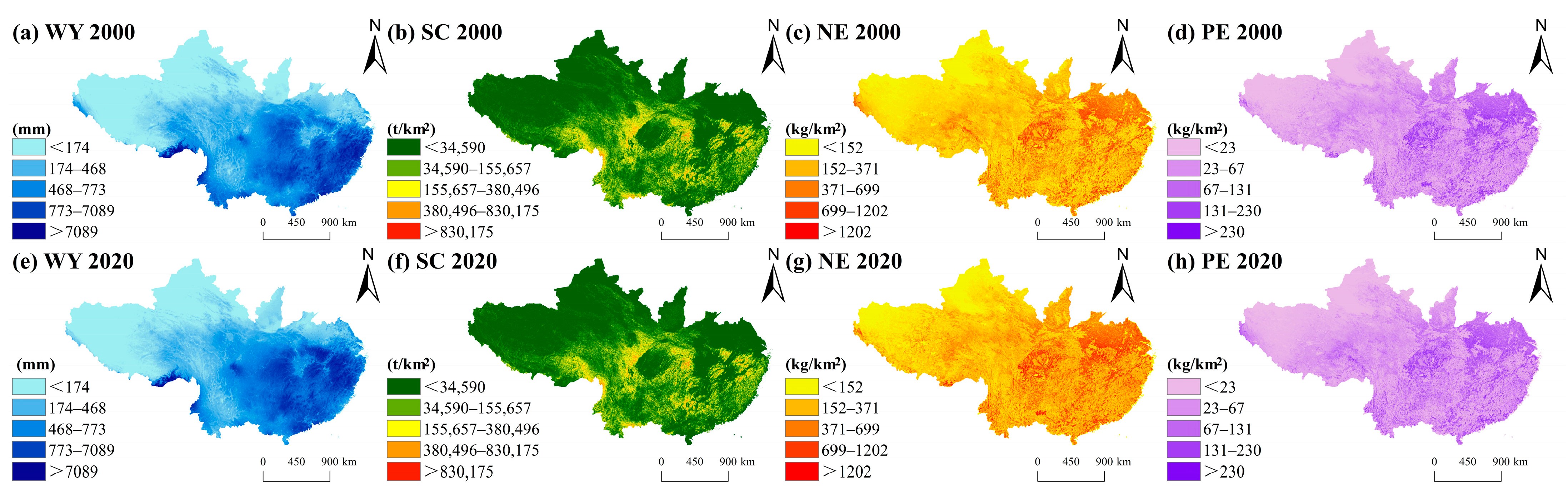
Basins play a crucial role in providing basic ecosystem services to human society by drawing clean freshwater from upstream sources to meet essential needs such as drinking water, agricultural irrigation, and domestic water supply [44]. However, LULC changes (urbanization, agricultural expansion, and deforestation), climate change (extreme hydrological events), pollution emissions (industrialization, agricultural production, and domestic sewage discharge), and land degradation (over-exploitation, irrational agricultural activities, and deforestation) significantly impact the hydrologic cycle, water quantity, and water quality in river basins [45]. These changes can have significant impacts on the ESs provided by river basins, including reduced clean water supply, deteriorating water quality, increased soil erosion, and declining soil fertility [46]. Water yield (WY), a crucial parameter in hydrology and water resources management, determines the amount of water available for various purposes, such as drinking, irrigation, power generation, and ecosystem maintenance [47]. Soil conservation (SC) is a crucial parameter for maintaining agricultural productivity, ensuring food security, and preserving the natural environment [48]. Water purification (WP), an essential ecosystem service provided by river basins, involves the removal of pollutants and improvement of water quality through natural processes, thereby protecting human health and supporting the maintenance of water resources’ quality and quantity [49]. Therefore, three specific WESs factors have been selected for this paper, namely WY, SC, and WP.
Using InVEST 3.9.0 software [50], we assessed the WESs by incorporating the LULC, PRE, EVA, SER, DEM, annual precipitation erosivity, and vegetation available water content. Table 2 presents the biophysical coefficient parameters.

2.2.2. Water Yield

The InVEST model’s annual WY module presents a method for estimating water balance, which relies on precipitation, evaporation, LULC, plant-available water content, and root-restricting layer depth.
Y i = ( 1 A E T i P i ) × P i ,
where Yi represents the annual WY (mm) of each grid cell i, AETi is the actual annual precipitation (mm/yr), and Pi denotes the annual precipitation (mm/yr).
The root mean square error between the model value (as in Table 3) and the observed is minimized at 50.13 when the parameter Z = 0.86.

2.2.3. Soil Conservation

The sediment delivery ratio (SDR) module in the InVEST model computes the Universal Soil Loss Equation (USLE) for each image pixel using the USLE.
R K L S x = R x K x L S x ,
U S R L x = R x K x L S x C x P x ,
S C x = R K L S x U S L E x ,
S C x = R x K x L S x ( 1 C x P x ) ,
where USRLx represents the average annual soil erosion; Rx denotes the rainfall coefficient; Kx indicates the soil erosion coefficient; LSx signifies the field topography coefficient; Cx represents the planting and management coefficient; Px indicates the coefficient of supporting conservation measures. The accuracy of the calculation results was validated by comparing them with the measured annual soil erosion in the experimental runoff area (Table 4).

2.2.4. Water Purification

WP is a crucial ecosystem service that focuses on the relative export of total dissolved nitrogen as an indicator of pollution. WP pertains to the capacity of ecosystems to alleviate water pollution by retaining certain non-point source pollutants through the actions of vegetation and soils. A significant impact of LULC on water quality is the presence of nutrients in surface water. The nitrogen export (NE) and phosphorus export (PE) per pixel in landscape x can be computed using Equations (5) and (6), respectively.
N E i = l o a d N i × N D R N i ,
P E i = l o a d P i × N D R P i ,
where NEi and PEi are the total amount of nitrogen and phosphorus exported, respectively; loadNi and loadPi are the nutrient loads of N and P, respectively; NDRNi and NDRPi are the nutrient delivery ratios of N and P, respectively. Due to the unavailability of measured data on PE and NE, the accuracy of the results was primarily achieved by referring to published model parameters within a specific region within the study area [51].

2.3. Framework of Correlation Analysis

This research provides a comprehensive analysis of both the natural ecosystem and the socio-economic system, exploring the spatial relationships of WESs supply and demand changes from 2000 to 2020 within the study area. It aims to elucidate the evolving characteristics of these patterns. Additionally, it investigates the dynamic correlation between changes in WESs supply and demand over time, exploring these correlations within distinct regions. The outlined research ideas and overall design are visually represented in Figure 2. This framework comprises three core components:
(1)
WESs supply calculation. Utilizing the Millennium Ecosystem Assessment (MA) framework alongside the Common International Classification of Ecosystem Services (CICES), this study selected vital WESs, specifically, WY, SC, and WP (as depicted in Table 5). Employing the respective ecological models, a spatial mapping approach was employed to compute the supply of these WESs from 2000 to 2020.
(2)
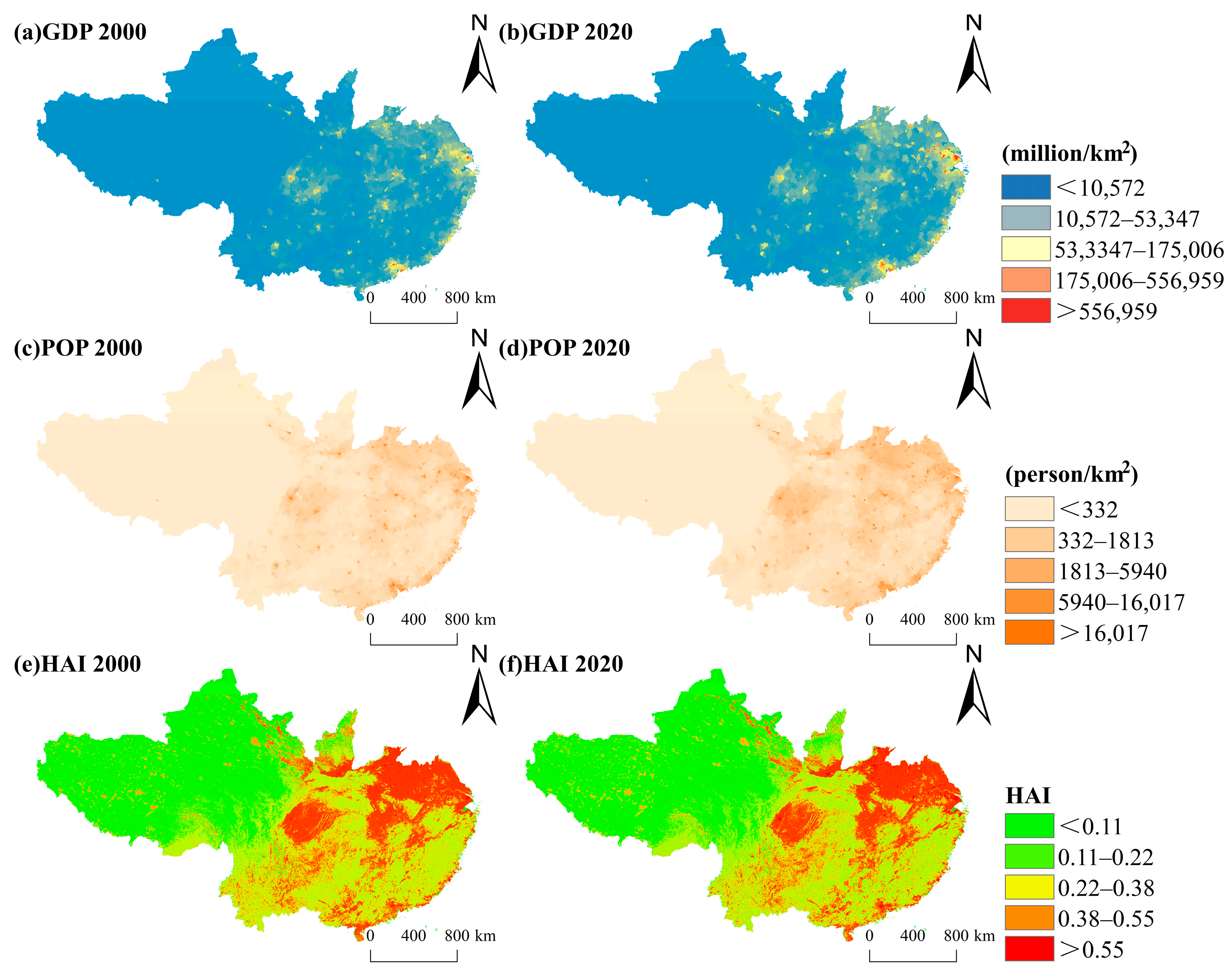
WESs demand calculation. Estimating WESs demand involves selecting three socio-economic indicators (HAI, POP, and GDP) to characterize and understand the demand for these services. Employing these indicators, spatial mapping of WESs demand within the study area was conducted, spanning the timeframe from 2000 to 2020.
(3)
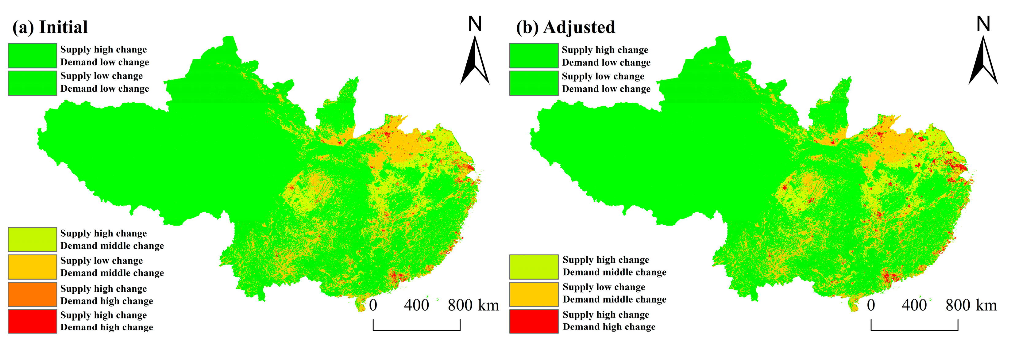
The study conducts spatial correlation analysis to examine the changes in both the supply and demand of WESs from a zoning perspective. This entails examining the spatial and temporal variations in the supply and demand of WESs in the study area from 2000 to 2020 by employing hotspot analysis to investigate the aggregation/dispersion patterns of supply change and demand change in the WESs. Ecological zoning is carried out based on these changes (categorized as high–medium–low) by overlaying the hotspot analysis results of supply and demand changes. The OPGD method is utilized to analyze the factors affecting different WESs and the relationship between their supply and demand changes in diverse zones. The factor detector is used to assess the impact of WESs demand changes on society, ecology, and nature, revealing the trend (positive/negative) of WESs demand changes on different WESs supply changes. Lastly, ecological management suggestions for balancing WESs supply and demand are proposed based on the spatial correlation of changes in WESs supply and demand across different zones.

2.4. Evaluating the Supply–Demand Relationship of WESs

2.4.1. Quantifying WESs Supply

Based on the natural geographic traits of the YRB and PRB and existing research [52,53,54], WY, WP, and SC were chosen as the WESs supply components. The calculation principles and formulas for these WESs are outlined in Section 2.2. Standardizing these three WESs using the Min–Max method and applying equal weights, their combined value was derived, considering the crucial significance of each WESs component.
According to the different dimensions of WESs, we normalized each WESs (WY, SC, NE, and PE) to a uniform value between 0 and 1 and then summed them to obtain the WESs for subsequent analyses [55], which were calculated as follows.
W E S s = i = 1 4 W E S s i , j W E S s i , min W E S s i , max W E S s i , min ,
where WESsi,j signifies the initial value of ecosystem service i in pixel j, while WESsi,min, and WESsi,max represent the minimum and maximum values of WESs, respectively.

2.4.2. Quantifying WESs Demand

Demand for ecosystem services pertains to the quantity of ESs anticipated or consumed by society [56]. Following the approach outlined in Peng et al. [55], we utilized population, LULC, and GDP as socio-economic indicators to define and understand the demand for WESs. LULC signifies the intensity of human water resource consumption. A higher ratio of construction to cropland indicates greater land development and utilization, thereby escalating water resource consumption. Population size serves as a reflection of the demand for WESs; heightened population density correlates with a higher overall demand for WESs. GDP mirrors the level of economic development in different regions, indirectly indicating the community’s inclination towards WESs. Elevated regional economic development aligns with higher expected WESs.
According to Xu et al. [17], the demand for WESs can be computed using the following equation:
E S D = x i 1 × lg ( x i 2 ) × lg ( x i 3 ) ,
where ESD is the demand for WESs and x i 1 , x i 2 , and x i 3 are the LULC intensity, POP (unit: person/km2), and GDP (unit: million/km2), respectively. According to Wu et al. [28], x i 1 was the intensity index of human activities (HAI). POP and GDP indicators were integrated into the calculation of WESs demand without affecting the overall distribution, using a logarithmic statistical approach that weakens localized sharp fluctuations to facilitate analysis. x i 1 was calculated as follows:
x i 3 = i = 1 n A i P i T A ,
where n corresponds to the number of LULC types; Ai represents the area of the i-th LULC type; TA denotes the total area; Pi signifies the intensity coefficient of human activities, reflecting the ecological value of the i-th LULC type, with values of 0.61 for cropland, 0.14 for forest land, 0.09 for grassland, 0.32 for water, 0.95 for construction, and 0.07 for unused land [57,58].

2.5. Optimal Parameters-Based Geographical Detector

Spatial heterogeneity and its underlying drivers can be identified using a GWR model [59]. Discretization of continuous variables is crucial for the application of this model, and the efficiency of discretization can be evaluated using the q statistic [60]. A higher q value indicates more significant spatial heterogeneity in the changes in WESs supply [61]. Traditionally, parameter settings are determined manually, which may introduce subjectivity. Consequently, we utilized the R programming environment to compute the q values for each continuous factor and apply various classification techniques, including quantiles, natural breaks, quartiles, and geometric intervals, with the number of intervals ranging from 3 to 9 classes [62,63,64]. Subsequently, we aimed to select a parameter combination (comprising classification method and number of intervals) that maximizes the q-value for spatial discretization.
q = 1 h = 1 L N h σ h 2 N σ 2 ,
where h represents the stratification (i.e., classification or partitioning) of variable Y or factor X, with a range of values from 1 to L; L represents the classification or partitioning of the various drivers. Nh and N denote the number of cells in stratified zone h and the entire zone, respectively. σ h 2 and σ 2 signify the variance of the h-zone and the overall regional variance of the Y value, respectively.

3. Results

3.1. WESs Spatial Pattern of Supply and Demand

By analyzing the spatial and temporal dynamics of the supply of each WESs from 2000 to 2020 (Figure 3), the high WY values are mainly distributed in the southeast and coastal regions. Higher SC values were found in Sichuan and Hubei provinces, while lower SC values were found in the western region. The NE and PE showed a pattern of high values in the central and northeastern regions and low values in the western region. From 2000 to 2020, spatial patterns changed little. From 2000 to 2020, overall WESs values were higher in the central and coastal mountainous areas, with a widening trend in the low values (Figure 4). Among them, the results of the Guangdong study in this paper are consistent with those of Xu et al. [17] in the Guangdong region.
The spatial and temporal dynamics of demand for various WESs are characterized by a significant increase in GDP from 2000 to 2020 (Figure 5). In 2000, the per capita GDP was only 2 × 10⁸ CNY/km2, whereas in 2020, it had surpassed 3 × 10⁹ CNY/km2. High-value areas are located mainly in the central and coastal areas. Areas with high population densities are mainly located in the coastal areas. From 2000 to 2020, there was a general trend of expansion. Land development intensity was highest in the northern and coastal regions. Construction increased significantly, by 50% or more. The demand for WESs is higher in the northern and coastal regions (Figure 6). Demand for WESs has increased dramatically in high-value areas along the coast.

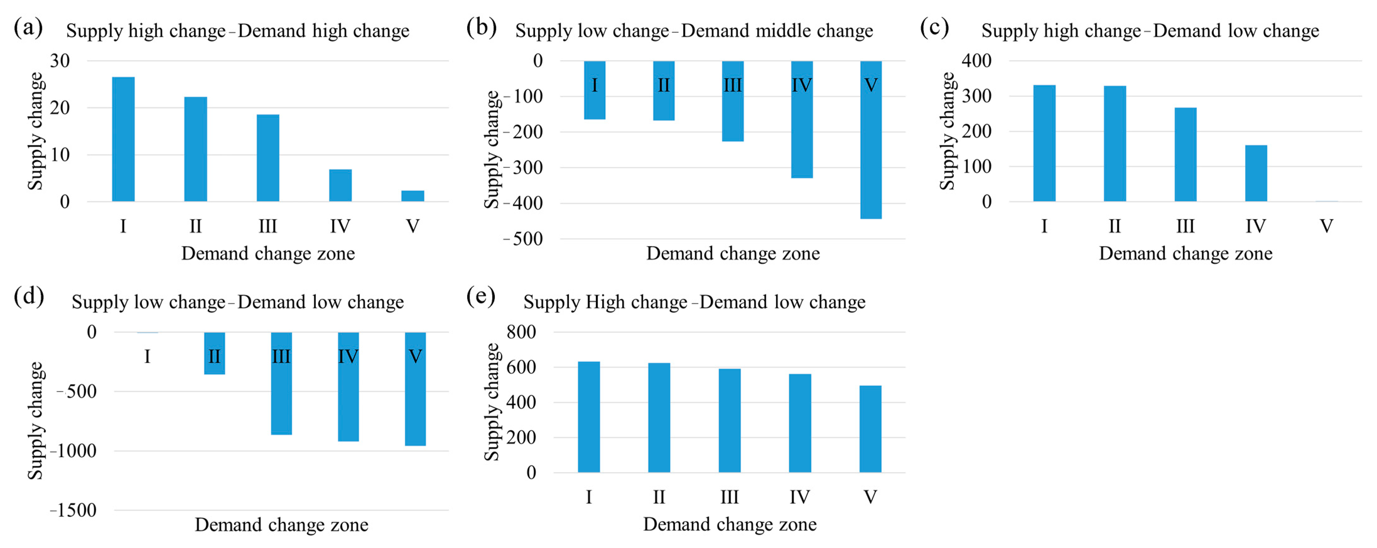
3.2. WESs Supply Change and Demand Change Zoning

This study examines the spatial evolution of changes in the supply and demand of WESs from 2000 to 2020 (Figure 7). The results show that the supply of WESs in the study area decreased significantly in coastal areas, while the supply of WESs in most other areas coexisted with increases and decreases. The demand for WESs shows a growing trend in coastal areas and developed cities, with rapid growth. Meanwhile, there was a slight increase in the demand for WESs in the northern mountainous regions. The spatial aggregation traits of changes in both the supply and demand of WESs support subsequent spatial zoning and governance efforts. Regarding the supply of WESs, the northern region stands out as a crucial cold spot area, whereas the central, northern, and Pearl River Delta regions emerge as notable hot spots. The demand for WESs has increased significantly, and Yunnan, Fujian, and other places are important cold spots.
When overlaying the shifts in supply and demand within the hot and cold areas for WESs and comparing the variations in supply changes among hot, unimportant, and cold spot areas, it was observed that the disparities between unimportant and cold spot areas were not substantial (Table 6). Therefore, these two regions were combined in the zoning. By comparing the difference in demand change of WESs in hotspot, insignificant, and coldspot regions, a significant difference between the three regions was found. Therefore, these three regions are independent and do not need to be merged.
Based on the above principles, the spatial changes in both the supply and demand of WESs were overlaid to derive their spatial pattern. The six types of changes in WESs supply and demand encompass scenarios like high supply change–low demand change, low supply change–low demand change, high supply change–middle demand change, low supply change–middle demand change, high supply change–high demand change, and low supply change–high demand change (Figure 8a). However, fewer of the regions exhibiting high supply change–high demand change and low supply change–high demand change within the studied areas (Table 7). These two types contribute to a relatively scattered zoning pattern and weaker zoning indicators overall. Following the principle of regional covariance and similarity in characteristics, the category of low supply change–high demand change was consolidated into the high supply change–high demand change classification.
After regional adjustment, the study area was divided into five WESs supply–demand change regions (Figure 8b). Areas characterized by high supply change–high demand change predominantly encompass coastal cities such as Shenzhen, Guangdong, Shanghai, and others, alongside the central city of Sichuan province, Chengdu. The alterations in WESs supply and demand within this region are typified by a substantial rise in both supply and demand for these services. Low supply change–middle demand change areas are mainly distributed in Henan, Anhui, and Shaanxi provinces. In this region, the changes in WESs supply exhibit minimal fluctuations, whereas there are moderate increments in the demand for WESs. Regions exhibiting high supply change and middle demand change are primarily distributed across Jiangsu, Anhui, Hubei, and Sichuan provinces. Within this region, the alterations in WESs supply indicate significant changes, while the demand for WESs experiences a moderate increase. The area characterized by low supply change and low demand change is concentrated in the western region. This region exhibits minimal alterations in both the supply and demand of WESs. Areas displaying low supply change and high demand change are primarily concentrated in the YRB and PRB. Within this region, alterations in WESs supply indicate minimal changes, while there are significant increases in the demand for WESs.

3.3. Correlation between WESs Supply Change and Demand Change

Before delving deeper into the spatial correlation of supply and demand changes in WESs, we first focused on analyzing the impacts of various socio-economic and natural factors on the supply changes in different types of WESs (Table 7). The natural factor PRE is the main driver of supply changes in WY. Soil is the primary influencing factor for SC supply changes, followed by HAI. For WP supply changes, the HAI factor has a more significant impact on WP supply changes compared to the natural factor, followed by CLP and GLP.
In studying the spatial correlation of supply and demand changes in WESs, it can be observed that there are significant differences in the degree to which changes in WESs supply are influenced by changes in WESs demand across different zones. In all zones, changes in WESs supply are significantly affected by changes in WESs demand (Table 8). In the high supply–low demand zone and the low supply–low demand zone, WY has the highest explanatory power for WESs demand changes (0.275), indicating that PRE has the greatest impact on WESs demand change. From the high supply–middle demand zone to the low supply–middle demand zone and then to the high supply–high demand zone, PE explanatory power for WESs demand changes gradually increases. It can be seen that as WESs demand starts from middle levels and HAI gradually dominates WESs demand changes. At the same time, the downward trend in WESs supply significantly affected by WESs demand change continues to increase across all zones (Figure 9), suggesting that an increase in WESs demand change will have a negative impact on WESs supply change.

4. Discussion

4.1. Influencing Factors of the Correlation between WESs Supply and Demand Changes

The influence of LULC changes on the variations in the supply and demand of WESs has been extensively acknowledged across diverse studies [65,66]. In the Southern River Basin, the overall characteristics of LULC changes reveal a significant increase in construction alone (Figure 10). In the high supply–high demand zone, all types of LULC changes are transformed into construction areas, with the area of construction increasing from 9208 km2 in 2000 to 29,412 km2. The expansion of construction areas has brought severe human disturbances to natural ecosystems, posing significant threats that may endanger the living environments of various organisms within these ecosystems [67]. In the high supply–high demand zone, the areas of natural ecosystems such as cropland, forest land, grassland, and water have all decreased, thereby limiting the supply level of WESs. Chen et al. [68] also reported the same results. In the high supply–high demand zone, the areas of grassland and unused land are the least, decreasing to 90 km2 and 169 km2, respectively. Forest land, grassland, and water only increase in the low-demand zone of WESs. Cropland increases in the middle demand zone. Wang et al. [69] have also demonstrated that during periods of stable economic growth, the area of cropland gradually increases. However, when the economy experiences rapid growth, the cropland area is damaged, primarily due to the continuous increase in construction areas. From Table 8 and Figure 9, it can be observed that the changes in the supply of various WESs in all zones are significantly affected by changes in WESs demand. When the changes in WESs demand exceed the middle level, the extent of influence of HAI, FLP, and GLP on WESs demand becomes increasingly larger. At the same time, the area of construction increases the most in the high supply–high demand zone. Therefore, the intensification of LULC changes may amplify the impact of WESs demand on WESs supply.
From the perspective of zoning, changes in WESs demand will significantly affect the changes in PE supply in each zone. From the high supply–middle demand zone to the low supply–middle demand zone and then to the high supply–high demand zone, PE has a significant impact on WESs demand changes. The middle demand and high demand zones mainly include the core areas of the Yangtze River Delta and the Pearl River Delta, including megacities such as Shanghai, Wuhan, Guangdong, and Chongqing, which are also key areas for sewage discharge [70]. For example, in 2015, the total amount of wastewater discharged in the YRB was 34.67 billion tons, of which 15.12 billion tons were domestic sewage and 19.55 billion tons were industrial wastewater (Yangtze River Basin Rural Statistics Yearbook, 2015). Among the 82 representative sewage outlets monitored in Guangdong, 29 exceeded the discharge standards, with the main pollutants being chemical oxygen demand, total phosphorus, and ammonia nitrogen (Guangdong Rural Statistics Yearbook, 2020). Therefore, rapid urbanization has led to a large amount of sewage discharge, worsening water quality and exacerbating the contradiction between WP supply and demand.

4.2. Policy Implications

Currently, policy is primarily focused on mitigating and adapting to climate change in the Southern River Basin. Mitigation measures primarily focus on stabilizing and reducing the concentration of greenhouse gases in the atmosphere. This approach aims to decelerate the pace of climate change by controlling emissions of greenhouse gases and optimizing the energy structure through adjustments [71]. For example, at the United Nations Climate Change Conference, India proposed aiming for net-zero emissions by the year 2070. Additionally, they committed to advancing emissions reductions and enhancing energy efficiency by accelerating the adoption and production of new energy vehicles. Adaptation measures primarily focus on alleviating the adverse effects and potential risks brought about by climate change. These measures involve bolstering the identification and management of risks associated with natural ecosystems and socio-economic systems [72]. China has enacted the National Climate Change Adaptation Strategy 2035, with a focus on enhancing the nation’s capacity to adapt to climate change. This strategy is aimed at achieving this goal through national water-saving initiatives, the establishment of a water resources monitoring system, and the reinforcement of water infrastructure construction [73]. Scientific research predominantly centers on examining the impact of climate change, emphasizing the need for implementing adaptation policies in regions facing imbalances between water supply and demand. This consensus underscores the urgency of addressing climate change impacts in such areas [74,75,76].
The study identified that the primary cause behind the escalating imbalance of WESs in the Southern River Basin is the surge in human activities, surpassing the impact of climate change. Hence, alongside pursuing climate adaptation policies, it is imperative to pay heightened attention to the issue of growing imbalances in WESs driven by the rapid expansion of human activities. The regional surge in population, economic advancement, and swift urbanization translate into amplified demand for ecosystem services, notably water resources. Consequently, this heightened demand leads to a decreased supply of WESs. Simultaneously, the rapid expansion of human activity downstream signifies a heightened dependence on available supplies. Firstly, it is imperative to decelerate the rapid growth of human activities. This involves strategies such as controlling population growth, establishing judicious urban expansion boundaries, coordinating the expansion of irrigated agriculture, and advocating for economic transformation. Secondly, by enhancing the urban water structure and enhancing agricultural irrigation efficiency, it is possible to mitigate the adverse impacts of human activities. These efforts are key to maintaining the equilibrium of WESs. By managing high population growth rates, harmonizing urban and rural development, and advocating for economic transformation, we can regulate water demand within a manageable range. This, in turn, reduces reliance on upstream water supply. Furthermore, optimizing urban water usage structure and enhancing agricultural irrigation efficiency can mitigate the adverse effects of escalating human activities in the future, leading to sustainable development.

4.3. Limitations and Prospects

In comparison to existing research on WESs supply and demand, the most prominent innovation of this study lies in its robust objectivity, dynamism, comparability, non-subjectivity, suitability, and transferability. Firstly, unlike traditional subjective methods for selecting WESs elements, this study chooses four categories of WESs elements based on literature analysis (Section 2.2.1), thereby demonstrating strong objectivity and laying a solid foundation for the research. Secondly, unlike previous studies on WESs supply and demand that only considered the relationship for a single year, this research takes into account the impact of dynamic changes in WESs supply and demand, leading to more dynamic and scientific experimental results. Thirdly, previous studies have only considered administrative or natural attributes. In contrast, this research proposes a novel perspective by treating the Southern River Basin sub-basins as a whole and preserving both social and natural attributes at the grid scale. This approach enables an evaluation of the supply and demand relationship of WESs in the Southern River Basin, making it more comparable. Fourthly, through comparisons between different zones, OPGD overcomes the influence of human subjectivity and enhances the study of dynamic changes in WESs supply and demand. Fifthly, the methodological framework employed in this research exhibits strong suitability, and we demonstrated its applicability to the analysis of WESs supply and demand changes in other research fields.
This study does come with certain limitations. First, the quantitative assessment of WESs demand relies on three indicators, GDP, POP, and HAI, suggesting similar requirements for various WESs. This uniformity might hinder accurate characterization and mapping of WESs supply. To better quantify each WESs supply, diverse methods should be employed. Additionally, while computing the total supply of the WESs, an equal-weighted superposition calculation approach was used for the four WESs. This method might diminish the important differences among the different WESs within the study area. Identifying the overall changes in the past 20 years within a two-year period poses a significant challenge. Future research should further examine the supply–demand relationships of WESs across multiple temporal scales. Conducting an in-depth analysis of the mechanisms influencing changes in WESs supply and demand could provide significant insights into their impact.

5. Conclusions

The interdependence between the supply and demand of WESs is evident, highlighting their close relationship. Understanding this intrinsic connection proves beneficial in aligning the natural ecosystem with the socio-economic system, fostering sustainable regional development. In this study, the supply and demand of WESs in both 2000 and 2020 were mapped for the Southern River Basin, serving as an illustrative example. Ecological zoning was conducted by considering the evolving traits of WESs supply and demand. Additionally, the correlation between changes in the supply and demand of WESs across distinct zones was investigated using the OPGD.
The main conclusion is that: the characteristics of WESs supply and demand changes exhibit spatial heterogeneity. The growth of WESs demand exceeds the growth of WESs supply. Based on the changes in WESs supply and demand, the Southern River Basin can be further divided into five zones: high supply change–low demand change, low supply change–low demand change, high supply change–middle demand change, low supply change–middle demand change, and high supply change–high demand change. In all zones, the changes in the supply of all types of WESs are significantly affected by changes in WESs demand. In the high supply–low demand zone, WY has the highest explanatory power for WESs demand changes (0.275). From the high supply–middle demand zone to the low supply–middle demand zone, and then to the high supply–high demand zone, the explanatory power of PE for WESs demand changes gradually increases. It can be seen that as WESs demand starts from the middle level, HAI gradually dominates the changes in WESs demand. In all zones, an increase in WESs demand changes will have a negative impact on WESs supply changes. Changes in LULC and intensified LULC alterations may exacerbate the impact of changes in WESs demands on supply. This study effectively incorporates the supply and demand changes of WESs and their correlations into the ecological protection and restoration governance system. Therefore, we have empirically explored the intrinsic relationship between WESs supply and demand changes. Based on this, future research can further focus on the key paths and links of multi-regional, multiscale, long-term WESs supply and demand correlations.

Author Contributions

Conceptualization, Yuncheng Jiang and Zhigang Yan; methodology, Yuncheng Jiang; software, Zhigang Yan and Bin Ouyang; validation, Yuncheng Jiang and Bin Ouyang; formal analysis, Yuncheng Jiang; investigation, Yuncheng Jiang and Bin Ouyang; resources, Yuncheng Jiang and Bin Ouyang; data curation, Yuncheng Jiang; writing—original draft, Yuncheng Jiang and Zhigang Yan; writing—review and editing, Yuncheng Jiang, Zhigang Yan, and Bin Ouyang; supervision, Zhigang Yan and Bin Ouyang; project administration, Zhigang Yan and Yuncheng Jiang; funding acquisition, Zhigang Yan. All authors have read and agreed to the published version of the manuscript.

Funding

This study was financially supported by the National Natural Science Foundation of China (41971370), the Fundamental Research Funds for the Central Universities (2023XSCX045), the Graduate Innovation Program of China University of Mining and Technology (2023WLKXJ163), the Postgraduate Research and Practice Innovation Program of Jiangsu Province (KYCX23_2751), the China Scholarship Fund ((2023) 49), and the 2022 Annual Science and Technology Research Project of Jiangxi Provincial Education Department (GJJ2206615).

Institutional Review Board Statement

Not applicable.

Informed Consent Statement

Not applicable.

Data Availability Statement

The data presented in this study are available from the authors upon reasonable request.

Acknowledgments

We would like to express our sincere thanks to the reviewers and editors for their valuable comments that helped improve this paper.

Conflicts of Interest

The authors declare no conflicts of interest.

References

  1. Costanza, R.; De Groot, R.; Sutton, P.; Van der Ploeg, S.; Anderson, S.J.; Kubiszewski, I.; Farber, S.; Turner, R.K. Changes in the global value of ecosystem services. Glob. Environ. Chang. 2014, 26, 152–158. [Google Scholar] [CrossRef]
  2. Daily, G.C. (Ed.) . Nature’s Services: Societal Dependence on Natural Ecosystems; Island Press: Washington, DC, USA, 1997; Available online: http://refhub.elsevier.com/S0169-204600221-8/h0055 (accessed on 11 November 2023).
  3. De Groot, R.S.; Alkemade, R.; Braat, L.; Hein, L.; Willemen, L. Challenges in integrating the concept of ecosystem services and values in landscape planning, management and decision making. Ecol. Complex. 2010, 7, 260–272. [Google Scholar] [CrossRef]
  4. Xue, Q.; Yang, X.; Wu, F. A three-stage hybrid model for the regional assessment, spatial pattern analysis and source apportionment of the land resources comprehensive supporting capacity in the Yangtze River Delta urban agglomeration. Sci. Total Environ. 2020, 711, 134428. [Google Scholar] [CrossRef] [PubMed]
  5. Miao, Z.; Baležentis, T.; Tian, Z.; Shao, S.; Geng, Y.; Wu, R. Environmental performance and regulation effect of China’s atmospheric pollutant emissions: Evidence from “three regions and ten urban agglomerations”. Environ. Resour. Econ. 2019, 74, 211–242. [Google Scholar] [CrossRef]
  6. Liu, C.F.; Wang, C.; Liu, L.C. Spatio-temporal variation on habitat quality and its mechanism within the transitional area of the Three Natural Zones: A case study in Yuzhong county. Geogr. Res. 2018, 37, 419–432. Available online: https://www.mdpi.com/1099-4300/20/6/419 (accessed on 11 November 2023).
  7. Wood, S.L.; Jones, S.K.; Johnson, J.A.; Brauman, K.A.; Chaplin-Kramer, R.; Fremier, A.; Girvetz, E.; Gordon, L.J.; Kappel, C.V.; Mandle, L.; et al. Distilling the role of ecosystem services in the Sustainable Development Goals. Ecosyst. Serv. 2018, 29, 70–82. [Google Scholar] [CrossRef]
  8. Costanza, R.; De Groot, R.; Braat, L.; Kubiszewski, I.; Fioramonti, L.; Sutton, P.; Farber, S.; Grasso, M. Twenty years of ecosystem services: How far have we come and how far do we still need to go? Ecosyst. Serv. 2017, 28, 1–6. [Google Scholar] [CrossRef]
  9. Desai, B.H. 14. United Nations Environment Program (UNEP). 2015. Available online: http://refhub.elsevier.com/S0169-204600221-8/h0180 (accessed on 11 November 2023).
  10. Assessment, M.E. Millennium Ecosystem Assessment. 2001. Available online: http://chapter.ser.org/europe/files/2012/08/Harris.pdf (accessed on 11 November 2023).
  11. UNCCD (United Nations Convention to Combat Desertification). Poor Land Use Costs Countries 9 Percent Equivalent of Their GDP; UNCCD: Bonn, Germany, 2018; Available online: https://www.unccd.int/news-events/poor-land-use-costs-countries-9-percentequivalent-their-gdp (accessed on 11 November 2023).
  12. Zhai, T.; Wang, J.; Jin, Z.; Qi, Y.; Fang, Y.; Liu, J. Did improvements of ecosystem services supply-demand imbalance change environmental spatial injustices? Ecol. Indic. 2020, 111, 106068. [Google Scholar] [CrossRef]
  13. Bakker, K. Water security: Research challenges and opportunities. Science 2012, 337, 914–915. [Google Scholar] [CrossRef]
  14. Liu, W.; Zhan, J.; Zhao, F.; Yan, H.; Zhang, F.; Wei, X. Impacts of urbanization-induced land-use changes on ecosystem services: A case study of the Pearl River Delta Metropolitan Region, China. Ecol. Indic. 2019, 98, 228–238. [Google Scholar] [CrossRef]
  15. Bi, Y.; Zheng, L.; Wang, Y.; Li, J.; Yang, H.; Zhang, B. Coupling relationship between urbanization and water-related ecosystem services in China’s Yangtze River economic Belt and its socio-ecological driving forces: A county-level perspective. Ecol. Indic. 2023, 146, 109871. [Google Scholar] [CrossRef]
  16. Yang, S.; Bai, Y.; Alatalo, J.M.; Wang, H.; Jiang, B.; Liu, G.; Chen, J. Spatio-temporal changes in water-related ecosystem services provision and trade-offs with food production. J. Clean. Prod. 2021, 286, 125316. [Google Scholar] [CrossRef]
  17. Xu, Z.; Peng, J.; Dong, J.; Liu, Y.; Liu, Q.; Lyu, D.; Qiao, R.; Zhang, Z. Spatial correlation between the changes of ecosystem service supply and demand: An ecological zoning approach. Landsc. Urban Plan. 2022, 217, 104258. [Google Scholar] [CrossRef]
  18. Zagonari, F. Using ecosystem services in decision-making to support sustainable development: Critiques, model development, a case study, and perspectives. Sci. Total Environ. 2016, 548, 25–32. [Google Scholar] [CrossRef]
  19. Xu, Z.; Wei, H.; Fan, W.; Wang, X.; Huang, B.; Lu, N.; Ren, J.; Dong, X. Energy modeling simulation of changes in ecosystem services before and after the implementation of a Grain-for-Green program on the Loess Plateau—A case study of the Zhifanggou valley in Ansai County, Shaanxi Province, China. Ecosyst. Serv. 2018, 31, 32–43. [Google Scholar] [CrossRef]
  20. Sun, R.; Li, F.; Chen, L. A demand index for recreational ecosystem services associated with urban parks in Beijing, China. J. Environ. Manag. 2019, 251, 109612. [Google Scholar] [CrossRef]
  21. Qiu, S.; Peng, J.; Dong, J.; Wang, X.; Ding, Z.; Zhang, H.; Mao, Q.; Liu, H.; Quine, T.A.; Meersmans, J. Understanding the relationships between ecosystem services and associated social-ecological drivers in a karst region: A case study of Guizhou Province, China. Prog. Phys. Geogr. Earth Environ. 2021, 45, 98–114. [Google Scholar] [CrossRef]
  22. Wu, X.; Liu, S.; Zhao, S.; Hou, X.; Xu, J.; Dong, S.; Liu, G. Quantification and driving force analysis of ecosystem services supply, demand and balance in China. Sci. Total Environ. 2019, 652, 1375–1386. [Google Scholar] [CrossRef] [PubMed]
  23. Peng, J.; Wang, X.; Liu, Y.; Zhao, Y.; Xu, Z.; Zhao, M.; Wu, J. Urbanization impact on the supply-demand budget of ecosystem services: Decoupling analysis. Ecosyst. Serv. 2020, 44, 101139. [Google Scholar] [CrossRef]
  24. Baró, F.; Gómez-Baggethun, E.; Haase, D. Ecosystem service bundles along the urban-rural gradient: Insights for landscape planning and management. Ecosyst. Serv. 2017, 24, 147–159. [Google Scholar] [CrossRef]
  25. Chen, X.; Li, F.; Li, X.; Hu, Y.; Hu, P. Evaluating and mapping water supply and demand for sustainable urban ecosystem management in Shenzhen, China. J. Clean. Prod. 2020, 251, 119754. [Google Scholar] [CrossRef]
  26. Liang, J.; Li, S.; Li, X.; Li, X.; Liu, Q.; Meng, Q.; Lin, A.; Li, J. Trade-off analyses and optimization of water-related ecosystem services (WRESs) based on land use change in a typical agricultural watershed, southern China. J. Clean. Prod. 2021, 279, 123851. [Google Scholar] [CrossRef]
  27. Liu, Y.; Yang, Y.; Wang, Z.; An, S. Quantifying Water Provision Service Supply, Demand, and Spatial Flow in the Yellow River Basin. Sustainability 2022, 14, 10093. [Google Scholar] [CrossRef]
  28. Wu, D.; Zheng, L.; Wang, Y.; Gong, J.; Li, J.; Chen, Q. Characteristics of urban expansion in megacities and its impact on water-related ecosystem services: A comparative study of Chengdu and Wuhan, China. Ecol. Indic. 2024, 158, 111322. [Google Scholar] [CrossRef]
  29. Li, J.; Xie, B.; Gao, C.; Zhou, K.; Liu, C.; Zhao, W.; Xiao, J.; Xie, J. Impacts of natural and human factors on water-related ecosystem services in the Dongting Lake Basin. J. Clean. Prod. 2022, 370, 133400. [Google Scholar] [CrossRef]
  30. Huang, L.; Chen, X.; Ye, C.; Yuan, Z.; He, K. Multiscale effects and drivers of landscape heterogeneity for water-related ecosystem services in urban agglomerations. Hydrol. Process. 2024, 38, e15081. [Google Scholar] [CrossRef]
  31. Liu, H.; Hou, L.; Kang, N.; Nan, Z.; Huang, J. A meta-regression analysis of the economic value of grassland ecosystem services in China. Ecol. Indic. 2022, 138, 108793. [Google Scholar] [CrossRef]
  32. Zhang, W. Constructing ecological interaction networks by correlation analysis: Hints from community sampling. Netw. Biol. 2011, 1, 81. Available online: https://www.researchgate.net/profile/Wenjun-Zhang-10/publication/228560951_Constructing_ecological_interaction_networks_by_correlation_analysis_Hints_from_community_sampling/links/575435f108ae10d9337a0dfb/Constructing-ecological-interaction-networks-by-correlation-analysis-Hints-from-community-sampling.pdf (accessed on 16 November 2023).
  33. Raiesi, F.; Beheshti, A. Evaluating forest soil quality after deforestation and loss of ecosystem services using network analysis and factor analysis techniques. Catena 2022, 208, 105778. [Google Scholar] [CrossRef]
  34. Sun, J.; Li, Y.P.; Gao, P.P.; Suo, C.; Xia, B.C. Analyzing urban ecosystem variation in the City of Dongguan: A stepwise cluster modeling approach. Environ. Res. 2018, 166, 276–289. [Google Scholar] [CrossRef]
  35. Abdullah, A.Y.; Biswas, R.K.; Chowdhury, A.I.; Billah, S.M. Modeling soil salinity using direct and indirect measurement techniques: A comparative analysis. Environ. Dev. 2019, 29, 67–80. [Google Scholar] [CrossRef]
  36. Luo, L.; Mei, K.; Qu, L.; Zhang, C.; Chen, H.; Wang, S.; Di, D.; Huang, H.; Wang, Z.; Xia, F.; et al. Assessment of the Geographical Detector Method for investigating heavy metal source apportionment in an urban watershed of Eastern China. Sci. Total Environ. 2019, 653, 714–722. [Google Scholar] [CrossRef] [PubMed]
  37. Belsti, Y.; Moran, L.; Du, L.; Mousa, A.; De Silva, K.; Enticott, J.; Teede, H. Comparison of machine learning and conventional logistic regression-based prediction models for gestational diabetes in an ethnically diverse population; the Monash GDM Machine learning model. Int. J. Med. Inform. 2023, 179, 105228. [Google Scholar] [CrossRef] [PubMed]
  38. Liu, S.; Shi, H.; Niu, J.; Chen, J.; Kuang, X. Assessing future socioeconomic drought events under a changing climate over the Pearl River basin in South China. J. Hydrol. Reg. Stud. 2020, 30, 100700. [Google Scholar] [CrossRef]
  39. Fang, Z.; Chen, J.; Liu, G.; Wang, H.; Alatalo, J.M.; Yang, Z.; Mu, E.; Bai, Y. Framework of basin eco-compensation standard valuation for cross-regional water supply–A case study in northern China. J. Clean. Prod. 2021, 279, 123630. [Google Scholar] [CrossRef]
  40. Zhang, Y.; Sun, M.; Yang, R.; Li, X.; Zhang, L.; Li, M. Decoupling water environment pressures from economic growth in the Yangtze River Economic Belt, China. Ecol. Indic. 2021, 122, 107314. [Google Scholar] [CrossRef]
  41. Zheng, Y.; He, Y.; Chen, X. Spatiotemporal pattern of precipitation concentration and its possible causes in the Pearl River basin, China. J. Clean. Prod. 2017, 161, 1020–1031. [Google Scholar] [CrossRef]
  42. Zhang, B.; Yin, J.; Jiang, H.; Chen, S.; Ding, Y.; Xia, R.; Wei, D.; Luo, X. Multi-source data assessment and multi-factor analysis of urban carbon emissions: A case study of the Pearl River Basin, China. Urban Clim. 2023, 51, 101653. [Google Scholar] [CrossRef]
  43. Bryan, B.A.; Ye, Y.; Connor, J.D. Land-use change impacts on ecosystem services value: Incorporating the scarcity effects of supply and demand dynamics. Ecosyst. Serv. 2018, 32, 144–157. [Google Scholar] [CrossRef]
  44. Jury, W.A.; Vaux, H.J., Jr. The emerging global water crisis: Managing scarcity and conflict between water users. Adv. Agron. 2007, 95, 1–76. [Google Scholar]
  45. Shrestha, S.; Bhatta, B.; Shrestha, M.; Shrestha, P.K. Integrated assessment of the climate and landuse change impact on hydrology and water quality in the Songkhram River Basin, Thailand. Sci. Total Environ. 2018, 643, 1610–1622. [Google Scholar] [CrossRef] [PubMed]
  46. Du Preez, C.C.; Van Huyssteen, C.W. Threats to soil and water resources in South Africa. Environ. Res. 2020, 183, 109015. [Google Scholar] [CrossRef] [PubMed]
  47. Rasul, G. Food, water, and energy security in South Asia: A nexus perspective from the Hindu Kush Himalayan region. Environ. Sci. Policy 2014, 39, 35–48. [Google Scholar] [CrossRef]
  48. Qi, X.; Wang, R.Y.; Li, J.; Zhang, T.; Liu, L.; He, Y. Ensuring food security with lower environmental costs under intensive agricultural land use patterns: A case study from China. J. Environ. Manag. 2018, 213, 329–340. [Google Scholar] [CrossRef]
  49. Mohsen, M.S. Water strategies and potential of desalination in Jordan. Desalination 2007, 203, 27–46. [Google Scholar] [CrossRef]
  50. Sharp, R.; Douglass, J.; Wolny, S.; Arkema, K.; Bernhardt, J.; Bierbower, W.; Chaumont, N.; Denu, D.; Fisher, D.; Glowinski, K.; et al. InVEST 3.9. 0. post195+ ug. gbc51afe User’s Guide; The Natural Capital Project; Stanford University: Stanford, CA, USA, 2020. [Google Scholar]
  51. Jiang, Y.; Ouyang, B.; Yan, Z. Multiscale Analysis for Identifying the Impact of Human and Natural Factors on Water-Related Ecosystem Services. Sustainability 2024, 16, 1738. [Google Scholar] [CrossRef]
  52. Fan, F.; Liu, Y.; Chen, J.; Dong, J. Scenario-based ecological security patterns to indicate landscape sustainability: A case study on the Qinghai-Tibet Plateau. Landsc. Ecol. 2021, 36, 2175–2188. [Google Scholar] [CrossRef]
  53. Fu, B.; Ouyang, Z.; Shi, P.; Fan, J.; Wang, X.; Zheng, H.; Zhao, W.; Wu, F. Current condition and protection strategies of Qinghai-Tibet Plateau ecological security barrier. Bull. Chin. Acad. Sci. 2021, 36, 1298–1306. [Google Scholar] [CrossRef]
  54. Zhang, S.; Yang, P.; Xia, J.; Wang, W.; Cai, W.; Chen, N.; Hu, S.; Luo, X.; Li, J.; Zhan, C. Land use/land cover prediction and analysis of the middle reaches of the Yangtze River under different scenarios. Sci. Total Environ. 2022, 833, 155238. [Google Scholar] [CrossRef]
  55. Peng, J.; Yang, Y.; Xie, P.; Liu, Y.X. Zoning for the construction of green space ecological networks in Guangdong Province based on the supply and demand of ecosystem services. Acta Ecol. Sin. 2017, 37, 4562–4572. [Google Scholar]
  56. Villamagna, A.M.; Angermeier, P.L.; Bennett, E.M. Capacity, pressure, demand, and flow: A conceptual framework for analyzing ecosystem service provision and delivery. Ecol. Complex. 2013, 15, 114–121. [Google Scholar] [CrossRef]
  57. Han, R.; Feng, C.C.; Xu, N.; Guo, L. Spatial heterogeneous relationship between ecosystem services and human disturbances: A case study in Chuandong, China. Sci. Total Environ. 2020, 721, 137818. [Google Scholar] [CrossRef]
  58. Li, L.; Zhu, L.Q.; Zhu, W.B.; Xu, S.B.; Li, Y.H.; Ma, H. The correlation between ecosystem service value and human activity intensity and its trade-offs—Take Qihe River basin for example. China Environ. Sci. 2020, 40, 365–374. [Google Scholar] [CrossRef]
  59. Yang, J.; Wang, J.; Xu, C.; Liu, Y.; Yin, Q.; Wang, X.; Wang, L.; Wu, Y.; Xiao, G. Rice supply flows and their determinants in China. Resour. Conserv. Recycl. 2021, 174, 105812. [Google Scholar] [CrossRef]
  60. Song, Y.; Wang, J.; Ge, Y.; Xu, C. An optimal parameters-based geographical detector model enhances geographic characteristics of explanatory variables for spatial heterogeneity analysis: Cases with different types of spatial data. GIScience Remote Sens. 2020, 57, 593–610. [Google Scholar] [CrossRef]
  61. Wang, J.; Xu, C. Geodetector: Principle and prospective. Acta Geogr. Sin. 2017, 72, 116–134. [Google Scholar]
  62. Huan, H.; Wang, J.; Teng, Y. Assessment and validation of groundwater vulnerability to nitrate based on a modified DRASTIC model: A case study in Jilin City of northeast China. Sci. Total Environ. 2012, 440, 14–23. [Google Scholar] [CrossRef]
  63. Chen, J.; Yang, S.T.; Li, H.W.; Zhang, B.; Lv, J.R. Research on geographical environment unit division based on the method of natural breaks (Jenks). Int. Arch. Photogramm. Remote Sens. Spat. Inf. Sci. 2013, 40, 47–50. [Google Scholar] [CrossRef]
  64. Maliqi, E.; Singh, S.K. Quantitative estimation of soil erosion using open-access earth observation data sets and erosion potential model. Water Conserv. Sci. Eng. 2019, 4, 187–200. [Google Scholar] [CrossRef]
  65. Felipe-Lucia, M.R.; Soliveres, S.; Penone, C.; Fischer, M.; Ammer, C.; Boch, S.; Allan, E. Land-use intensity alters networks between biodiversity, ecosystem functions, and services. Proc. Natl. Acad. Sci. USA 2020, 117, 28140–28149. [Google Scholar] [CrossRef]
  66. Zorrilla-Miras, P.; Palomo, I.; Gómez-Baggethun, E.; Martín-López, B.; Lomas, P.L.; Montes, C. Effects of land-use change on wetland ecosystem services: A case study in the Doñana marshes (SW Spain). Landsc. Urban Plan. 2014, 122, 160–174. [Google Scholar] [CrossRef]
  67. Im, R.Y.; Kim, J.Y.; Nishihiro, J.; Joo, G.J. 2020. Large weir construction causes the loss of seasonal habitat in riverine wetlands: A case study of the Four Large River Projects in South Korea. Ecol. Eng. 2020, 152, 105839. [Google Scholar] [CrossRef]
  68. Chen, W.; Chi, G.; Li, J. The spatial association of ecosystem services with land use and land cover change at the county level in China, 1995–2015. Sci. Total Environ. 2019, 669, 459–470. [Google Scholar] [CrossRef] [PubMed]
  69. Wang, Y.; Li, X.; Xin, L.; Tan, M. Farmland marginalization and its drivers in mountainous areas of China. Sci. Total Environ. 2020, 719, 135132. [Google Scholar] [CrossRef] [PubMed]
  70. Xiangmei, M.; Feifei, F.; Lifeng, W. Prediction of major pollutants discharge from wastewater in 31 cities of China. Sustain. Prod. Consum. 2021, 26, 54–64. [Google Scholar] [CrossRef]
  71. Colelli, F.P.; Emmerling, J.; Marangoni, G.; Mistry, M.N.; De Cian, E. Increased energy use for adaptation significantly impacts mitigation pathways. Nat. Commun. 2022, 13, 4964. [Google Scholar] [CrossRef]
  72. Aryal, J.P.; Sapkota, T.B.; Khurana, R.; Khatri-Chhetri, A.; Rahut, D.B.; Jat, M.L. Climate change and agriculture in South Asia: Adaptation options in smallholder production systems. Environ. Dev. Sustain. 2020, 22, 5045–5075. [Google Scholar] [CrossRef]
  73. Ministry of Ecology and Environment. The National Strategy for Climate Change Adaptation 2035. 2022. Available online: https://www.mee.gov.cn/xxgk2018/xxgk/xxgk03/202206/t20220613_985261.html (accessed on 19 November 2023).
  74. Kraaijenbrink, P.D.; Stigter, E.E.; Yao, T.; Immerzeel, W.W. Climate change decisive for Asia’s snow meltwater supply. Nat. Clim. Chang. 2021, 11, 591–597. [Google Scholar] [CrossRef]
  75. Wang, T.; Zhao, Y.; Xu, C.; Ciais, P.; Liu, D.; Yang, H.; Yao, T. Atmospheric dynamic constraints on Tibetan Plateau freshwater under Paris climate targets. Nat. Clim. Chang. 2021, 11, 219–225. [Google Scholar] [CrossRef]
  76. Sondershaus, F.; Moss, T. Your resilience is my vulnerability: ‘Rules in use’ in a local water conflict. Soc. Sci. 2014, 3, 172–192. [Google Scholar] [CrossRef]
Figure 1. The location and topographic layout of the study site. (a) Geographic positioning of the study site within China. (b) Distribution of LULC in the study site in 2020. (c) Elevation mapping of Southern River Basin sub-basin.
Ijgi 13 00068 g001
Figure 2. A structured framework is established to synchronize and harmonize the supply and demand of WESs.
Ijgi 13 00068 g002
Figure 3. Spatial distribution of supply of various types of WESs.
Ijgi 13 00068 g003
Figure 4. Spatial distribution of WESs supply.
Ijgi 13 00068 g004
Figure 5. Spatial distribution of demand for various types of WESs.
Ijgi 13 00068 g005
Figure 6. Spatial distribution of WESs demand.
Ijgi 13 00068 g006
Figure 7. Mapping the spatial patterns of WESs supply change and demand change.
Ijgi 13 00068 g007
Figure 8. Ecological zoning is influenced by changes in supply and demand for WESs.
Ijgi 13 00068 g008
Figure 9. Spatial relationship between change in supply for WESs and change in demand for WESs in different zones.
Ijgi 13 00068 g009
Figure 10. Evolution of LULC within distinct zones from 2000 to 2020.
Ijgi 13 00068 g010
Table 1. Sources and use of data collected in this paper.
Target LayerCriterion LayerIndicator LayerYearSpatial
Resolution
Data Resource
SuitabilityNatureDigital elevation model (DEM)202030 mhttp://www.gscloud.cn, accessed on 21 September 2023
Slope (SLO)2020Extracted from elevation
Aspect2020
Normalized difference vegetation index (NDVI)20201 kmhttps://www.resdc.cn, accessed on 11 October 2023
Net primary productivity (NPP)2020
Soil types (Soil)2020https://www.ncdc.ac.cn/portal, accessed on 1 October 2023
Soil erosion types (SER)2020
Distance to water source (DWA)2000, 2020http://www.openstreetmap.org, accessed on 6 October 2023
ClimateAnnual mean temperature (TEM)https://www.geodata.cn, accessed on 11 September 2023
Annual mean precipitation (PRE)
Annual mean evaporation (EVA)
Annual mean relative humidity (RHU)
Total annual evapotranspiration (EVA)
Direct normal irradiation (DNI)
Sunshine hours (SSD)
Land use and land cover (LULC)Percentage of cropland land (CLP)2000, 202030 mhttps://www.resdc.cn, accessed on 19 September 2023
Percentage of forest land (FLP)
Percentage of grassland (GLP)
Percentage of water area (WLP)
Percentage of construction (ConsP)1 kmThe percentage of land area designated for construction use in the region represents the characteristics of LULC composition.
CoordinationSocio-
economic
Population (POP)2000, 20201 kmhttps://www.worldpop.org, accessed on 23 September 2023
Nighttime lighting data (NLD)2000, 2020
Gross domestic product (GDP)2000, 2020
Traffic
location
Distance to government (DGO)2020http://www.openstreetmap.org, accessed on 6 October 2023
Distance to road (DRO)2020
Distance to highway (DHI)2020
Distance to train station (DTS)2020
Distance to hospital (DHO)2020
Distance to school (DSC)2020
Distance to bus stops (DBS)2020
Table 2. Biophysical coefficients in the InVEST models.
LULCRoot_depthKcLULC_vegUsle_cUsle_pLoad_nLoad_pEff_nEff_pCrit_len_nCrit_len_pProportion_subsurface_n
Cropland3001.110.30.215.51.730.250.2530300.4
Forest land3500110.00612.50.150.70.73003000.15
Grassland8000.710.02160.80.480.481501500.15
Water area11.050000.0010.0010.050.0530300.25
Construction10.43000111.80.050.0530300.3
Other land10.5001111.80.050.0530300.1
Table 3. Comparison between observed data and modeled data of annual water yield (mm/yr).
River 20002020
Xiangjiang RiverObserved data764.53641.02
Modeled data813.08625.07
Error rate/%−6.352.49
Zishui RiverObserved data243.33283.55
Modeled data222.86278.03
Error rate/%8.411.95
Dongting Lake BasinObserved data2184.812803.21
Modeled data2016.272667.79
Error rate/%7.714.83
The data employed in this research were obtained from the Changjiang and Southwest Rivers Water Resources Bulletin (http://www.cjw.gov.cn/zwzc/bmgb/, accessed on 22 November 2023).
Table 4. The comparison between the observed and computed values of the annual soil loss amount in 2015.
Measured ValueCalculated ValueError Rate/%
LULCSoil Loss/Tons·km−2·yr−1LULCSoil Loss/Tons·km−2·yr−1
Economic fruit tree1223.3Forest land1441.517.8
Greening grassland1162.624.0
Bare land1972.9−27.0
Average1452.9−0.8
The measured data are from the Lianhe runoff monitoring station (located at 111°22′ E, 27°03′ N). The area of each runoff field is 100 m2.
Table 5. Basis for selecting WESs indicators.
IndicatorBasis for Selecting Indicators
WYWY plays a crucial role in maintaining human life and well-being by serving as a foundational cornerstone for various life-sustaining activities.
SCSoil conservation is crucial for upholding ecological balance, ensuring food security, and fostering sustainable development.
WPResolving water pollution in the YRB is absolutely vital, particularly focusing on tackling pollution in lakes, reservoirs, and water bodies with high levels of nitrogen and phosphorus.
Table 6. Significant differences in WESs supply and demand changes in different zones.
SupplyDemand
Hot spot20,999.1912,666,110.17
Not significant1337.70345,383.50
Cold spot12,669.91333,017.28
Table 7. Factorization test results for coupling coordination.
WY-FactorsDTSDBSDRODSCDHODGODHIDNI
q statistic0.2631 **0.3743 **0.2421 **0.3787 **0.3709 **0.3701 **0.3743 **0.6486 **
WY-FactorsAspectDEMSEREVAGDPNDVINLDNPP
q statistic0.1478 **0.5474 **0.5634 **0.3628 **0.4612 **0.4604 **0.4327 **0.6138 **
WY-FactorsPOPPRERHUSLOSoilSSDTEMDWA
q statistic0.4992 **0.8925 **0.7331 **0.0402 **0.5678 **0.6940 **0.5735 **0.0500 **
WY-FactorsCLPFLPGLPWLPConsPHAI
q statistic0.5148 **0.5547 **0.6234 **0.5713 **0.5342 **0.5182 **
SC-FactorsDTSDBSDRODSCDHODGODHIDNI
q statistic0.0325 **0.0739 **0.0445 **0.0747 **0.0813 **0.0775 **0.0739 **0.1089 **
SC-FactorsAspectDEMSEREVAGDPNDVINLDNPP
q statistic0.0188 **0.1169 **0.1534 **0.0359 **0.1097 **0.1256 **0.1437 **0.1338 **
SC-FactorsPOPPRERHUSLOSoilSSDTEMDWA
q statistic0.1348 **0.1379 **0.1530 **0.2296 **0.2362 **0.0737 **0.0510 **0.0235 **
SC-FactorsCLPFLPGLPWLPConsPHAI
q statistic0.2233 **0.2284 **0.2045 **0.1939 **0.1953 **0.2301 **
NE-FactorsDTSDBSDRODSCDHODGODHIDNI
q statistic0.1590 **0.2066 **0.2235 **0.2603 **0.2618 **0.2568 **0.2066 **0.2409 **
NE-FactorsAspectDEMSEREVAGDPNDVINLDNPP
q statistic0.0563 **0.2647 **0.2504 **0.1794 **0.2507 **0.1932 **0.2684 **0.2511 **
NE-FactorsPOPPRERHUSLOSoilSSDTEMDWA
q statistic0.2805 **0.2692 **0.2464 **0.0321 **0.1910 **0.2394 **0.2481 **0.0342 **
NE-FactorsCLPFLPGLPWLPConsPHAI
q statistic0.3263 **0.2696 **0.3310 **0.2473 **0.2463 **0.3501 **
PE-FactorsDTSDBSDRODSCDHODGODHIDNI
q statistic0.1626 **0.2110 **0.2368 **0.2691 **0.2699 **0.2610 **0.2110 **0.2191 **
PE-FactorsAspectDEMSEREVAGDPNDVINLDNPP
q statistic0.0483 **0.2736 **0.2554 **0.1631 **0.2622 **0.1714 **0.2809 **0.2370 **
PE-FactorsPOPPRERHUSLOSoilSSDTEMDWA
q statistic0.2930 **0.2194 **0.2151 **0.0552 **0.1960 **0.2080 **0.2233 **0.0367 **
PE-FactorsCLPFLPGLPWLPConsPHAI
q statistic0.3475 **0.2942 **0.3571 **0.2644 **0.2799 **0.3866 **
Note: ** represent significance.
Table 8. Calculation and analysis of correlation coefficients for changes in supply and demand of WESs.
WESsHigh Supply–Low Demand ZoneLow Supply–Low Demand ZoneHigh Supply–Middle Demand ZoneLow Supply–Middle Demand ZoneHigh Supply–High Demand Zone
WY0.275 **0.275 **0.245 **0.225 **0.158 **
SC0.259 **0.240 **0.224 **0.217 **0.169 **
NE0.240 **0.240 **0.231 **0.235 **0.252 **
PE0.226 **0.244 **0.301 **0.323 **0.421 **
Note: ** represent significance.
Disclaimer/Publisher’s Note: The statements, opinions and data contained in all publications are solely those of the individual author(s) and contributor(s) and not of MDPI and/or the editor(s). MDPI and/or the editor(s) disclaim responsibility for any injury to people or property resulting from any ideas, methods, instructions or products referred to in the content.

