Abstract
The seamless integration of indoor and outdoor positioning has gained considerable attention due to its practical implications in various fields. This paper presents an innovative approach aimed at detecting and delineating outdoor, indoor, and transition areas using a time series analysis of Global Navigation Satellite System (GNSS) error statistics. By leveraging this contextual understanding, the decision-making process between GNSS-based and Visual-Inertial Odometry (VIO) for trajectory estimation is refined, enabling a more robust and accurate positioning. The methodology involves three key steps: proposing the division of our context environment into a set of areas (indoor, outdoor, and transition), exploring two methodologies for the classification of space based on a time series of GNSS error statistics, and refining the trajectory estimation strategy based on contextual knowledge. Real data across diverse scenarios validate the approach, yielding trajectory estimations with accuracy consistently below 10 m.
1. Introduction
Positioning and geolocalization have been significant challenges that humans have sought to address since the dawn of civilisation. Technological advancements made in the last century have empowered 21st-century citizens to determine their location like never before. However, further progress is still necessary. One of the most relevant challenges is achieving seamless indoor–outdoor positioning on a global scale [1]. This requires a single positioning device capable of providing a reliable solution in any environment, whether it be outdoors or indoors.
On one hand, outdoor tracking technologies are well-established through GNSS [2]. The integration of GNSS into smartphones, along with applications like Google Maps, incorporating georeferenced topographical and aerial or background maps, significantly facilitates people’s location and navigation [3]. Although the error of these GNSS systems is typically a few meters, it still provides a more than satisfactory model for its intended purpose: assisting users in reaching a destination within a city, whether it is a strategic site or any building. The advantage of using GNSS-based positioning is that it can be applied to all people moving in an outdoor space [4]. The problem arises when people move from outdoors to indoors because GNSS-based systems degrade their performance in these environments [5,6,7]. This occurs because GNSS signals cannot penetrate indoor spaces. Moreover, they may also significantly degrade position accuracy in outdoor environments due to the blockage of GNSS signal or multipath, especially in non-GNSS friendly areas such as urban or forested regions.
Although several approaches for indoor positioning exist in the literature and on the market (mainly radiofrequency-based), these are not suitable for worldwide indoor–outdoor tracking because they rely on infrastructure that may not be available everywhere [8]. Another infrastructure-independent approach is also being developed by the scientific community, aiming to determine trajectories in indoor spaces using camera(s) and IMU data. The most advanced solutions rely on Simultaneous Localization and Mapping (SLAM) or Visual Inertial Odometry (VIO) approaches but may suffer from positional drift in the absence of loop closures, limiting their practical applicability to some extent.
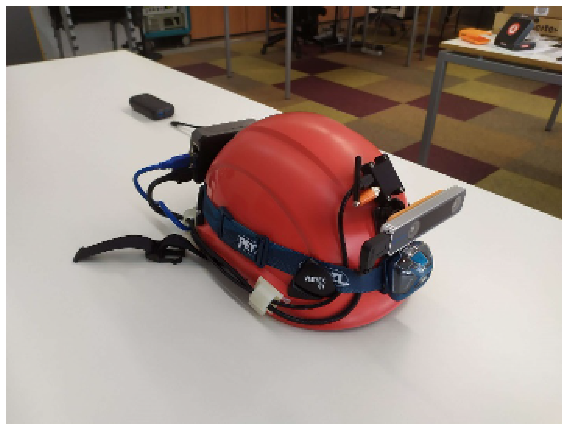
Approaches that integrate GNSS with SLAM-VIO-based methods have recently been investigated [9,10,11,12], but they are in the early stages. One recent effort in this direction is the work carried out in the IOPES project [8]. The research aimed to continuously track members of civil protection or emergency teams as they moved between outdoor and indoor areas. The authors believe that current technologies, encompassing both software and hardware, are robust enough to build a system capable of meeting the tracking requirements for emergency teams. This system would be based on data provided by IMUs, RGB-D cameras, and GNSS receivers [13], along with a suitable fusion algorithm. All these devices are installed on a helmet, and two trajectories are estimated in real-time, one based on the GNSS signal and the other one on the camera and IMU data, specifically relying on Visual Inertial Odometry (VIO) (Figure 1). Both trajectories are combined using a fusion algorithm to provide a single indoor–outdoor trajectory. The system predominantly relies on a GNSS-based solution for outdoor tracking and a VIO-based solution for indoor tracking [14].

Figure 1.
Positioning system mounted on a helmet designed and built by CTTC.
Although this work represents a significant step forward in seamless indoor–outdoor tracking performance, it remains insufficient. This limitation arises from the current approach, which relies solely on the most recent GNSS error statistic (such as horizontal GNSS accuracy error) to determine whether a person is indoors or outdoors, subsequently deciding on the most reliable trajectory between the GNSS-based or the VIO-based methods. Consequently, while the indoor and outdoor trajectories are accurate individually, the connection between the two lacks precision, potentially resulting in a substantial shift in indoor areas.
This paper introduces a novel approach to address this issue. We propose a method for detecting outdoor, indoor, and transition areas based on a time series of GNSS error statistics rather than relying on a single epoch. By utilising this accumulated contextual knowledge, we aim to improve the decision-making strategy for choosing between GNSS-based and VIO methods. The goal is to provide a more robust and accurate seamless indoor and outdoor trajectory.
The approach consists of three distinct steps. Firstly, a proposal to divide our contextual environment into a set of areas (indoor, outdoor, and transition). Then, the implementation and exploration of three methodologies for the classification of the space: one based on the most recent GNSS statistics and two based on a time series of GNSS error statistics. Finally, the seamless indoor–outdoor trajectory estimation approach is enhanced by integrating knowledge of the contextual environment. The feasibility of the approach has been verified by obtaining and analysing estimated trajectories using real data from various scenarios with distinct characteristics.
The main contribution of this paper can be summarised as follows:
- The introduction of an innovative approach for detecting outdoor, indoor, and transition areas through the time series analysis of GNSS error statistics.
- The refinement of the decision-making process between GNSS-based and Visual-Inertial Odometry (VIO) for trajectory estimation by leveraging contextual understanding.
- The validation of the approach using real data from diverse scenarios, demonstrating trajectory estimations with a consistent accuracy.
The rest of the paper is organised as follows: in Section 2, the scientific background is reported, which raises an objection to the context environment classification, and a proposal for its division are introduced; moreover, a description of the different methods developed and implemented in this paper are contextualised with recent research findings in Section 3. Then, Section 4 presents the different scenarios that have been used to evaluate the potential of the approach and the achieved results. In Section 5, the conclusions and further research are presented, together with a comparative analysis with existing methods.
2. Related Works
Several comprehensive reviews have been identified in the scholarly literature, emphasizing the critical need for integrated indoor–outdoor (IO) localization capabilities [15]. Scholars have explored various indoor and outdoor localization technologies, highlighting mechanisms for seamless transitions between environments without disrupting the localization process. Discussions include indoor localization technologies such as RFID [16], Ultra-Wide Band (UWB) [17], and Bluetooth Low Energy (BLE) [18], while outdoor localization is predominantly analyzed through GNSS.
For enhanced seamless positional accuracy, leveraging a hybrid fingerprinting approach that amalgamates data from multiple sensors is advocated over reliance on singular sensor systems. The adoption of fingerprinting techniques for seamless positioning has been elaborated upon in [17], where fingerprinting data are derived from either comprehensive or streamlined training databases. Techniques such as clustering, path-loss models, and image-based strategies are evaluated for their efficacy in contexts requiring range measurements. As shown in [19], Multi-Dimensional Scaling facilitates the transformation of high-dimensional data into a more manageable lower-dimensional format, accompanied by visual representation. Another important work [20] shows the effectiveness of localization techniques deployed on commercial smartphones, employing traditional methodologies such as proximity, Received Signal Strength (RSS), angle, timing, and map matching, noting their user-friendly advantage despite performance variability. Finally, in [21] IO localization advancements within the context of the Internet of Things (IoT) is shown, observing consistency in traditional localization methods alongside the introduction of novel approaches, notably LTE and 5G, for localizing entities like sensor nodes and drones in both two-dimensional and three-dimensional spaces.
However, it is worth noting that specific discussions on seamless IO localization— beyond mere differentiation between indoor and outdoor settings—are scarce, with a primary focus on technological methodologies and signal properties. Albeit the role of machine and deep learning in facilitating such adaptive, data-driven applications is deemed pivotal given their disruption, further investigation on data optimization with statistical techniques is mandatory.
Besides this gap, the literature shows that the definition of transition between indoor and outdoor needs clarification. In daily use, indoor and outdoor may seem clear, yet precisely defining them proves to be challenging. A review [22] compiles diverse spatial definitions from various fields. An increasing number of standards and applications are working towards three-dimensional notions to be able to represent parts of space. These aspects were investigated mainly because the key to link the outdoor/indoor trajectories is a function of the space due to the fact that the GNSS signal is influenced by the space [21].
A very dense canopy is another case where the GNSS signal may not be reliable, but there are also a lot of intermediate cases among open outdoor area and urban canyons [23] or dense forest areas [24]. So, it is natural to ask which is the limit; in terms of environment, we may consider an outdoor area with acceptable signal noise.
There are many studies presented in the literature regarding the definition of spaces in terms of navigation. Some define indoor spaces by physical boundaries [25,26], such as walls, doors, and windows, while others include underground spaces [27] or limit them to built environments [28].
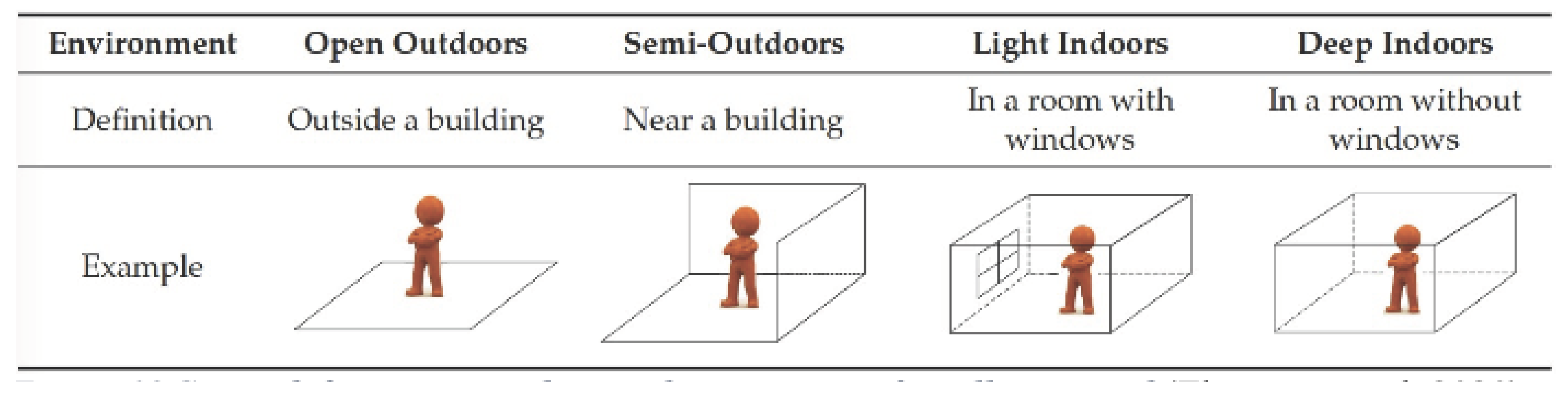
Few definitions address ambiguous semi-enclosed areas. Kray et al. [29] argue for a third transitional space alongside outdoor or indoor spaces. In terms of the reception of GNSS signal, the authors of [30] considered whatever was a GNSS-denied environment as indoor or semi-indoor, while the authors of [31] provided another classification of the areas: open outdoors, semi-outdoors, light indoors, and deep indoors as shown in Figure 2.
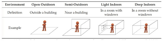
Figure 2.
Space definition proposed by [31] and adapted by [22].
Urban canyons and wooded areas are considered semi-outdoors. Light indoors resembles semi-outdoor spaces near windows with partial satellite availability. Deep indoors lack satellite coverage.
3. Methodology
3.1. Space Classification
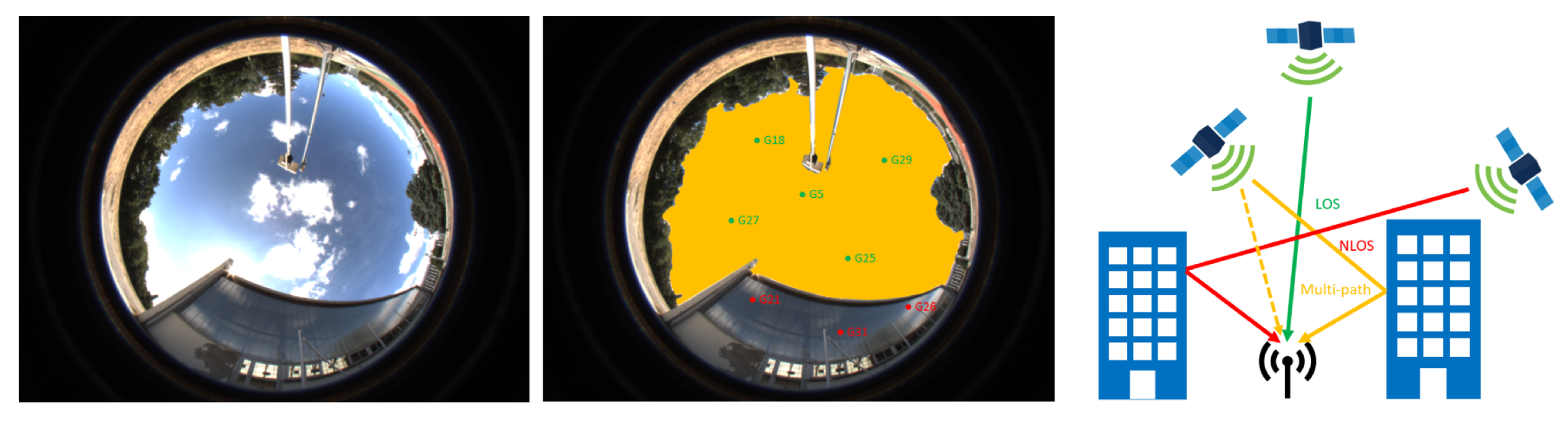
Initially, the approach that best suited our study was the one proposed by Wang [31], summarising how the GNSS signal might be affected by the surrounding space. In this approach, semi-outdoor serves as a transitional zone, merging light and deep indoor spaces into a single indoor area. GNSS errors arise when satellites are not directly visible, in other words, when they are Not in the Line Of Sight (NLOS) of that device, causing a multipath effect, which is a blend of direct and reflected signals (see Figure 3) [32]. Testing the GNSS in different spaces helps determine how it responds, aiding in defining semi-indoor and semi-outdoor limits. However, these limits fluctuate due to various factors such as satellite positions and weather, creating shifting boundaries rather than fixed lines.

Figure 3.
Left side: sky representation with projected satellites (green = LOS; red = NLOS). Right side: schemes of the multipath and NLOS effect [32].
Defining areas solely with GNSS signals for context detection proved challenging due to this complexity. In this context, the data available produced by a receiver and used in this research are as follows:
- Time of each point collected;
- Longitude, latitude, and height of each point collected;
- Horizontal error (H_err);
- Vertical error (V_err);
- Number of satellites.
Based on these parameters, in the following section three different procedures are presented to assign one of the following categories: indoor, outdoor, and transition area. The first one uses the most recent GNSS statistics (H_err and V_err), while the other approaches are based on a time series of GNSS-error estimation.
3.2. Determination of Indoor, Outdoor, and Transition Areas
3.2.1. Determination of Indoor, Outdoor, and Transition Areas Using GNSS Error Estimation
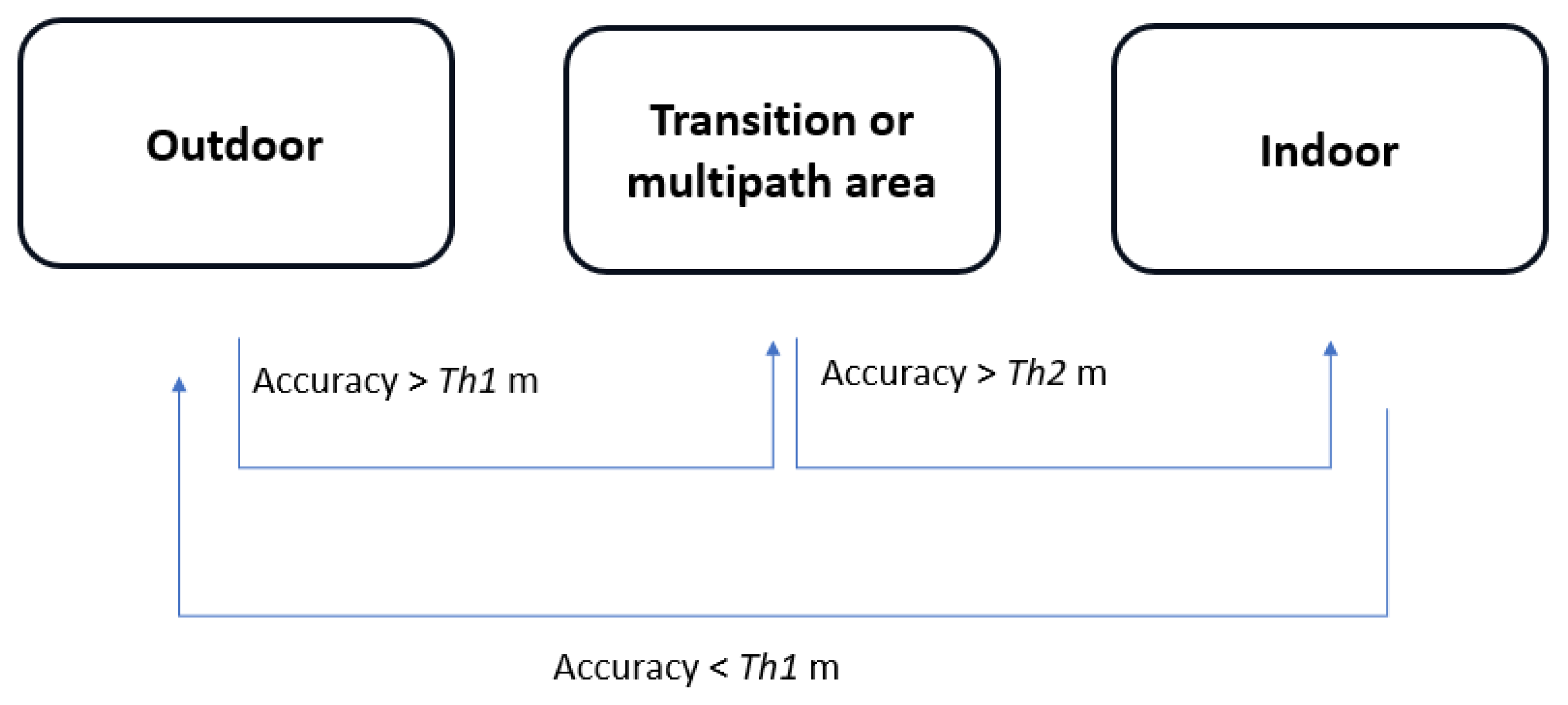
In the previous work [13], the method for detecting indoor and outdoor transitions relied on recent statistics (H_err and V_err) gathered by GNSS trajectories and two different thresholds (Th1 and Th2) (Figure 4). However, this approach encountered challenges when merging GNSS trajectories with VIO data, as highlighted in the introduction. The key to improving the combined trajectory is still hidden in the trajectory itself, so the trajectory data must be studied to obtain a trend that explains the behaviour of the GNSS in different spaces, and the algorithm must recognise the trend changes in time, otherwise linking a new trajectory to the GNSS one will result in substantial errors. These aspects will be explained in detail in the next paragraphs.
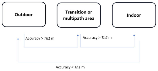
Figure 4.
Flowchart depicting the algorithm used to determine indoor, outdoor, and transition areas using the GNSS error estimation.
3.2.2. Determination of Indoor, Outdoor, and Transition Areas Using Time Series of GNSS Error Estimation—Slope Approach
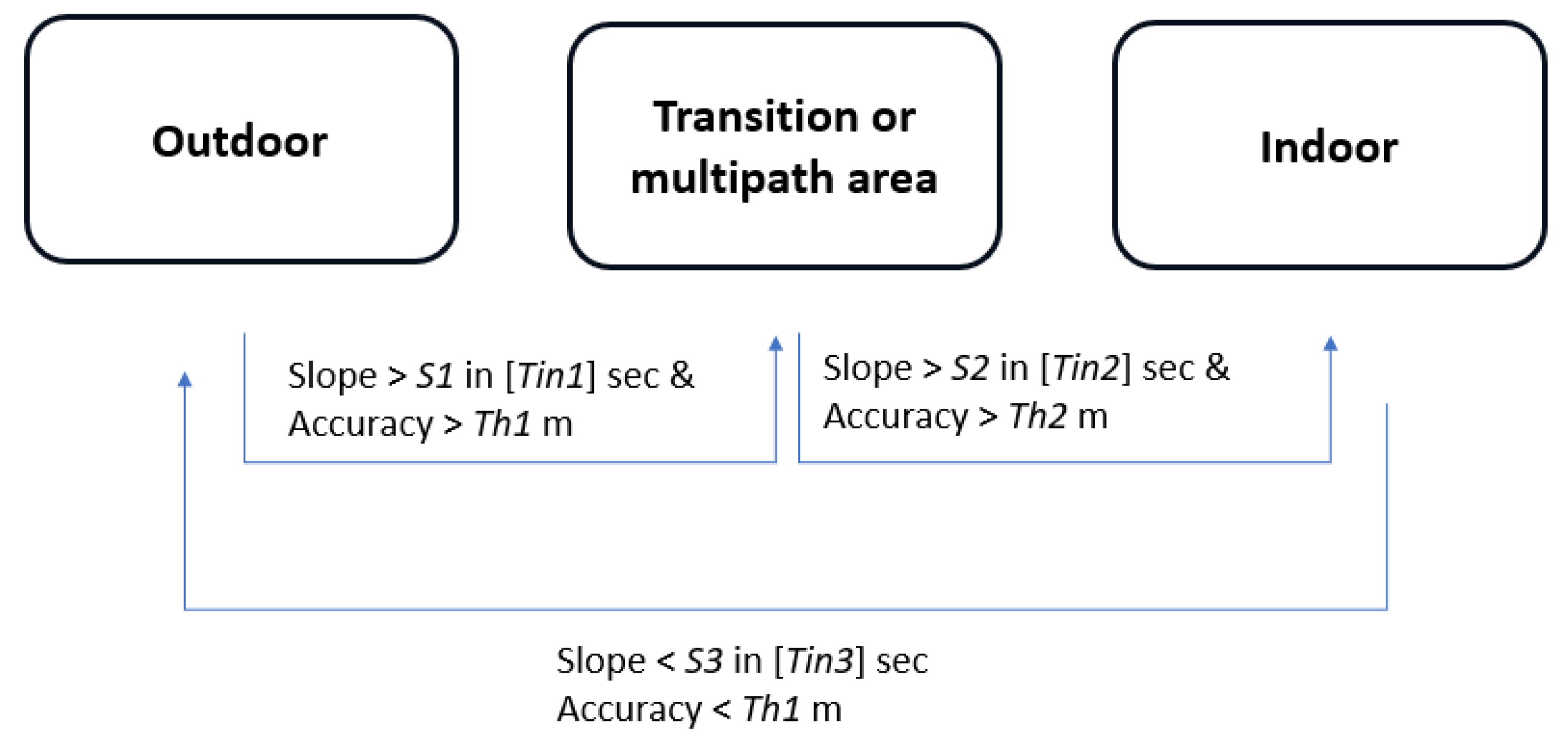
To establish a criterion for transitioning between GNSS- and VIO-based trajectories, the initial approach involves computing a slope from GNSS error statistics using a predefined n-size window. However, peaks may arise, particularly due to obstructions like trees, requiring rules to exclude these peaks while considering those near buildings or during entry indoors. Small obstacles, such as individual trees, briefly impact errors (denoted as Tin). Tin indicates the time to get in/out to/from the indoor area. Therefore, relying solely on a high horizontal or vertical slope (S) does not distinguish between approaching indoor areas or momentary obstacles. This emphasises the necessity for a transitional zone. Hereafter, the notation is as follows: Si stands for slope number i, Thi for threshold number i, and Tini for time to get in/out number i.
For instance, meeting conditions S1 within Tin1 seconds, with horizontal error exceeding Th1, suggests a non-deteriorating signal. Alternatively, exceeding S2 within Tin2 seconds, with higher accuracy, indicates entering an indoor area, differentiating from transitional zones. Failing these criteria implies remaining in an open outdoor area.
Determining the transition from indoor to outdoor might be complex. A slope lower than S3 during Tin3, which is a rapid horizontal error improvement, and overall error below Th1 signifies entry into reliable outdoor spaces. This algorithm is summarized in Figure 5.
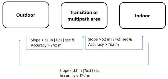
Figure 5.
Flowchart depicting the algorithm used to determine indoor, outdoor, and transition areas using the slope approach.
3.2.3. Determination of Indoor, Outdoor, and Transition Areas Using Time Series of GNSS Error Estimation—Mann–Kendall Test Approach
The Mann–Kendall statistical test (MK Test) is a non-parametric test [33,34] used for assessing the significance of trends [35]. It is mainly used for hydro-meteorological time series, and we assert that such a statistical test, despite there being no cases in the literature where this test has been used for similar purposes, could be fitting for this dataset. This is attributed to its compatibility with non-normally distributed data, its robustness against outliers in the data, and its capability to detect trends with relatively small sample sizes, as long as the data exhibit monotonic trends. A detailed description of the MK test can be found in Appendix A.
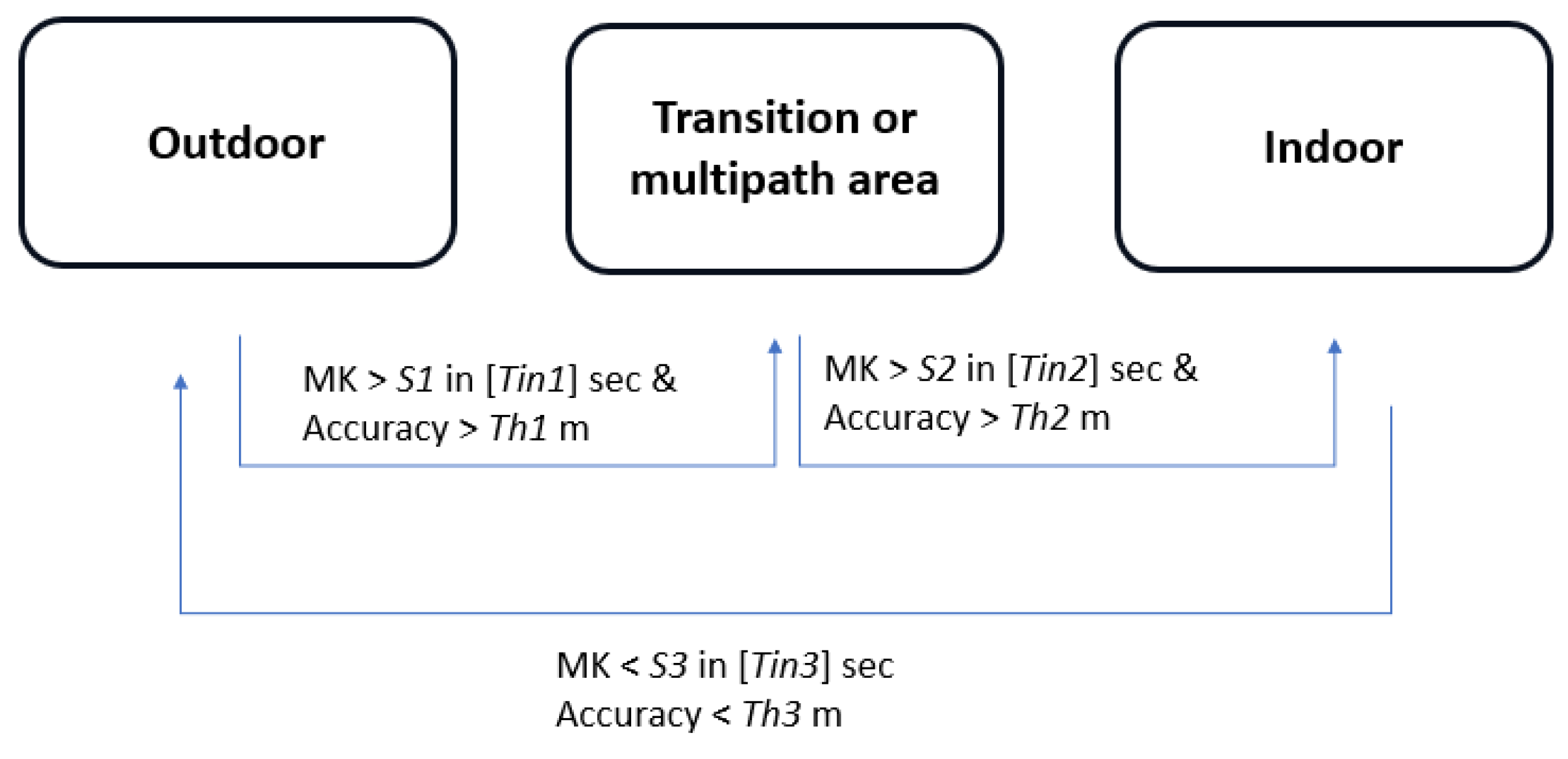
Having established this, we need to define a rule to switch between the different spaces. Similar to the prior scenario involving slope values, we establish the criteria described in Figure 6. In this approach, the MK statistical value (written as S in Appendix A) is used instead of the slope value.
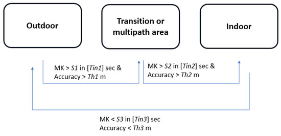
Figure 6.
Flowchart depicting the algorithm used to determine indoor, outdoor, and transition areas using the MK approach.
3.3. Seamless Indoor–Outdoor Trajectory Estimation
In order to compute a seamless indoor–outdoor trajectory, a data fusion algorithm that relates GNSS and camera-based positions, providing a single trajectory regardless of whether it originated indoors, outdoors, or both, has been adapted [8]. The tool has been modified to incorporate the determination of outdoor, transition, and indoor areas by introducing an external indicator as a new feature. The use of this indicator, derived from a time series of GNSS statistics, seeks to improve the selection criteria between using the GNSS-based or the VIO-based solution in each epoch, thus aiming to enhance the overall accuracy of the seamlessly estimated indoor–outdoor trajectory.
4. Results
4.1. Test Areas Description and Data Sources
Several campaigns were conducted to validate the performance of positioning sensors (visual-inertial odometry and GNSS sensors), to assess the efficacy of the approaches based on the time series of GNSS positions for detecting outdoor, indoor, and transition areas, and to evaluate the performance of the seamless indoor–outdoor positioning system. These campaigns spanned three locations in Catalonia (Spain): CTTC premises in Parc Mediterrani de la Tecnologia (Castelldefels) and its environs, Garraf town, and Collsuspina, each featuring indoor spaces, clear-sky areas, and locations with strong multipath conditions.
Five distinct routes were designated, encompassing various scenarios, including outdoor with clear sky, outdoor with low GNSS availability, and indoor spaces. The “PMT-LAB” route navigated a campus with multipath zones and indoor areas within different CTTC buildings. “Sa Falconera” explored Garraf’s surroundings, including cliff-side walks and tunnel passages. “Garraf Town” traversed narrow streets and concluded within a house showcasing four distinct rooms. Two routes in Collsuspina involved forest walks, cave exploration, and entry and exit from the building.
The prototype developed by [8] was used in these routes to acquire the positioning data. The positioning sensors that are included in the system are: a GNSS receiver that provides the GNSS-based trajectory, a stereo camera that provides the VIO-based trajectory, and a magnetometer. The system was mounted on a helmet (Figure 1), and a person walked through the routes while the positioning data were acquired and stored. Then, a seamless indoor–outdoor trajectory combining the GNSS and VIO-based trajectory was computed in post-processing. Although the system allows for real-time trajectory estimation, in this work, an offline and adapted version of the sensor fusion software approach of the system was used.
The “PMT-LAB” route facilitated a comprehensive analysis, evaluating GNSS error statistics and the performance of two algorithms for detecting outdoor, indoor, and transition areas. The remaining routes assessed the seamless indoor–outdoor trajectory estimation method’s performance and the detection of the detection of several areas using GNSS statistical time series data.
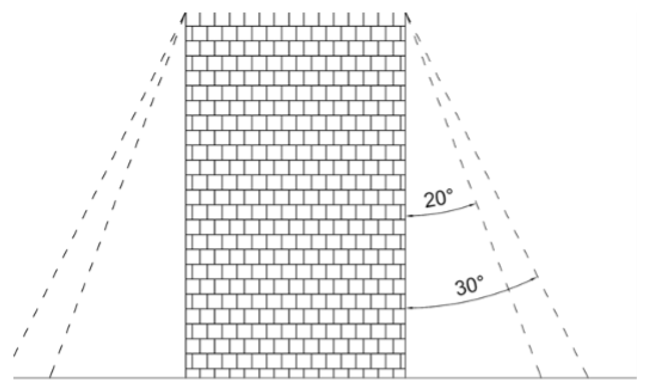
A very rough transition or semi-outdoor area was outlined along the “PMT-Lab” and “Garraf Town” routes, for aiding in the analysis of GNSS errors. This area was defined considering an angle of 20 degrees from the top of each building (Figure 7). A vectorial layer comprising the buildings of the area was generated using the Open Street Maps plugin in QGIS. The height information for each building was derived from a Digital Surface Model (DEM) provided by the Spanish Geographical National Institute, available for free at https://centrodedescargas.cnig.es (accessed on 1 February 2024). An example of this transition is is shown in Figure 8.

Figure 7.
Example of an area next to a building marked as transition or semi-outdoor area.

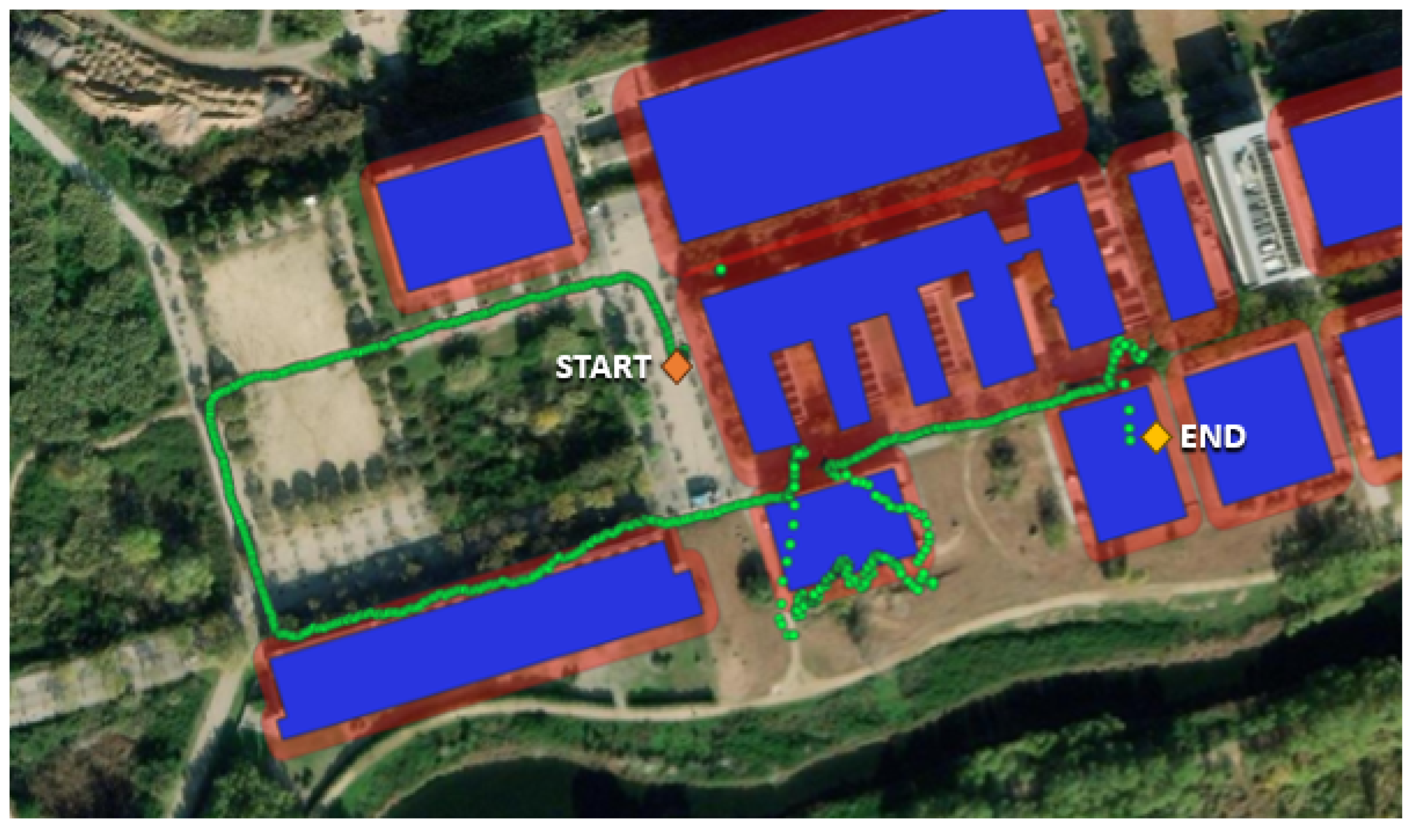
Figure 8.
Transition or semi-outdoor area for the “PMT-LAB” (red) and GNSS-based trajectory (green). Building layouts are shown in blue.
4.2. Determination of Areas Using GNSS Error Statistics
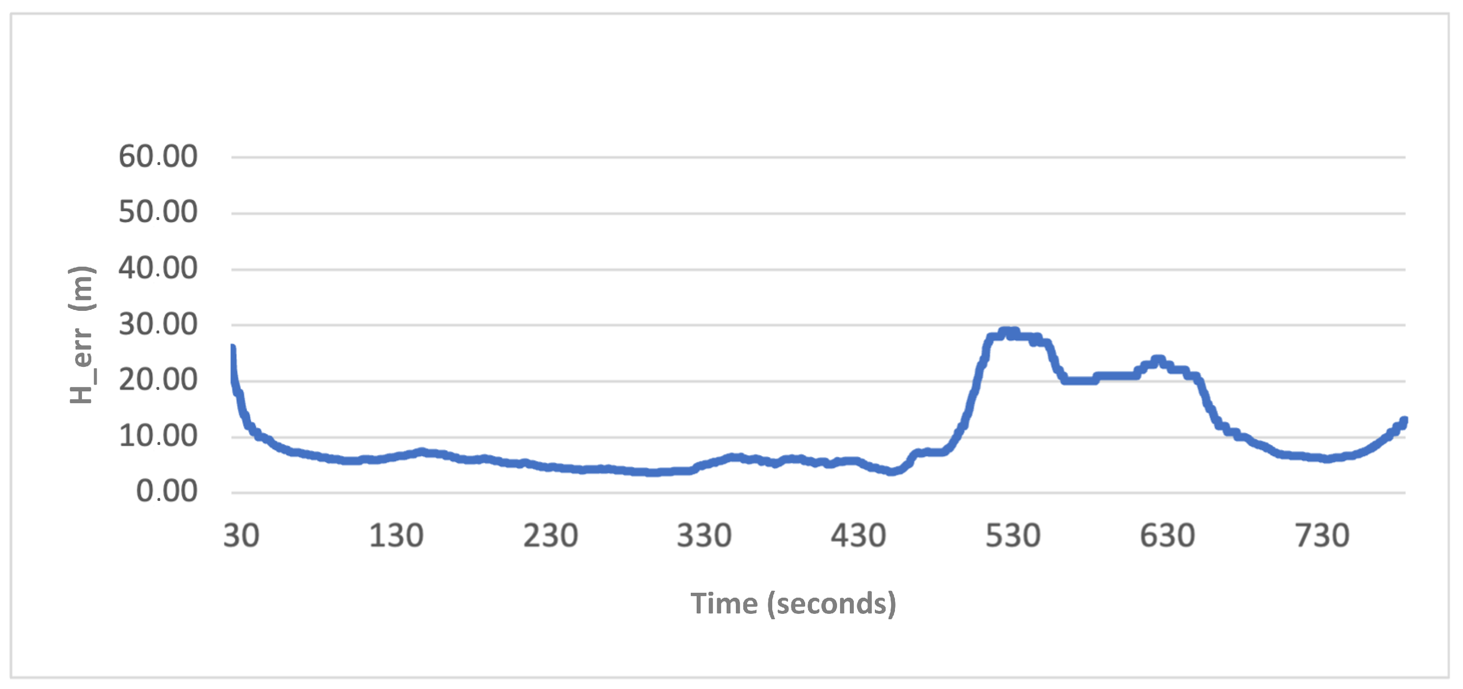
This section showcases the outcomes from analyzing indoor, outdoor, and transitional zones using the latest GNSS error statistics (H_err and V_err) along the “PMT-LAB” route. Figure 9 and Figure 10 exhibit the individual GNSS statistics’ horizontal and vertical errors to observe their behaviours. The horizontal error (H_err) emerged as the most dependable data for investigation (Figure 9). Figure 9 also shows some vertical lines, manually identified, corresponding to relevant events that occur such as entering or going out from transitional areas and buildings. In contrast, the vertical error (V_err) demonstrated relatively smoother changes in slope, making it less susceptible to rapid alterations over a short duration. However, this smoothness might obscure significant variations, complicating the identification of encountered obstacles, be it multipath zones or minor interferences like trees, causing signal noise (Figure 10).
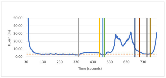
Figure 9.
GNSS trajectory horizontal error vs. time. Vertical lines highlight relevant events such as entering or going out from transitional areas and buildings. Horizontal orange line shows a a line with constant horizontal error of 5 m, while the horizontal green line shows of 3.5 m.

Figure 10.
GNSS trajectory vertical error vs. time.
Figure 9 and Figure 10 illustrate the initial convergence time required by the GNSS receiver after turning on. Once the error stabilizes, the graph maintains a nearly constant value of around 3.5 m. Notably, a significant deviation occurs around the second 342, just after the grey line. Here, the error increases slightly beyond 5 m and persists for approximately 130 s until the vertical yellow boundary. This deviation coincides with the trajectory near the building, where multipath results in an increase in the error. Consequently, after a few seconds, the estimated trajectory deviates from a straight line, failing to capture the real user’s path. The yellow line marks the conclusion of this initial obstacle. As expected, the horizontal error demonstrates improvement as the positioning device enters an open space, gradually stabilizing to values similar to those observed before encountering the first building.
Following the trajectory, two closely vertical positioned lines (blue and green) appear. The blue line denotes the boundary that supposedly marks the influence zone of the upcoming building, established at a 30-degree angle from the building’s top. In contrast, the green line marks the moment when the user approaches the entrance of this building. This approach, relying on thresholds derived from the last epoch of GNSS error statistics, reveals a major weakness. One would expect that a significant deviation in GNSS error indicators when the positioning device enters a building, highlighting that the GNSS-based solution is unreliable when switching to a VIO-based solution. However, the H_err displays only a marginal increase, similar to the earlier observed multipath effect. Although a 5-m error remains acceptable for estimating pedestrian trajectories, using an algorithm with these settings fails to guarantee a continuous and realistic trajectory.
The H_err values increase significantly when the device enters the building after several seconds. Consequently, relying solely on a simple approach like the H_err or its standard deviation in a specific area will result in switching to the VIO trajectory too late. This leads to erroneous positioning in that part of the trajectory, causing a loss of crucial information about the user’s indoor location while carrying the device. Similarly, the same issue arises when the user exits the building, indicated by the dark blue line in Figure 9. Although the GNSS signal becomes reliable upon exiting, it is imperative to switch to it instead of relying on the VIO trajectory, even though the H_err remains unstable at this point. This introduces another problem as a shifted VIO trajectory, considered incorrect, is utilised. The GNSS trajectory should be adopted as soon as the signal achieves reliability. However, defining these limits is still essential and requires understanding and establishment. A clear observation from the plot in Figure 9 is that using thresholds based solely on the last GNSS error statistics proves insufficient.
4.3. Determination of Areas Using GNSS Slope
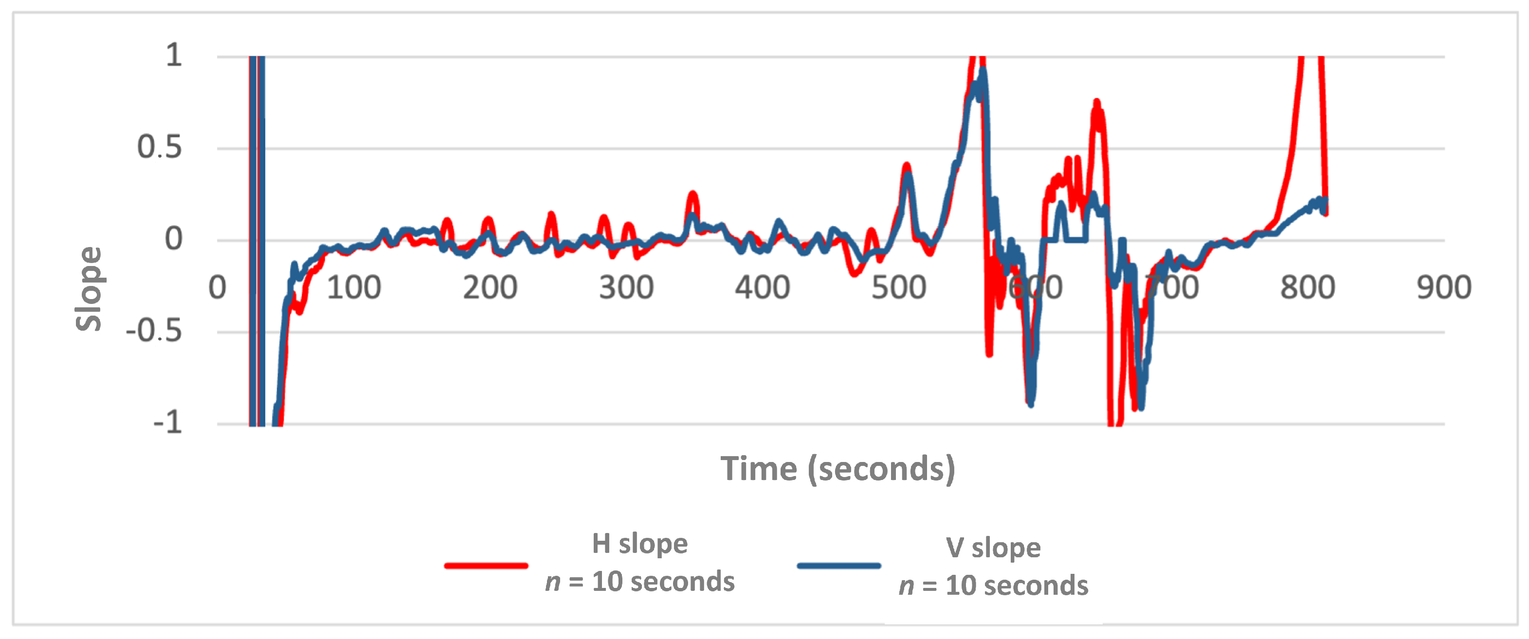
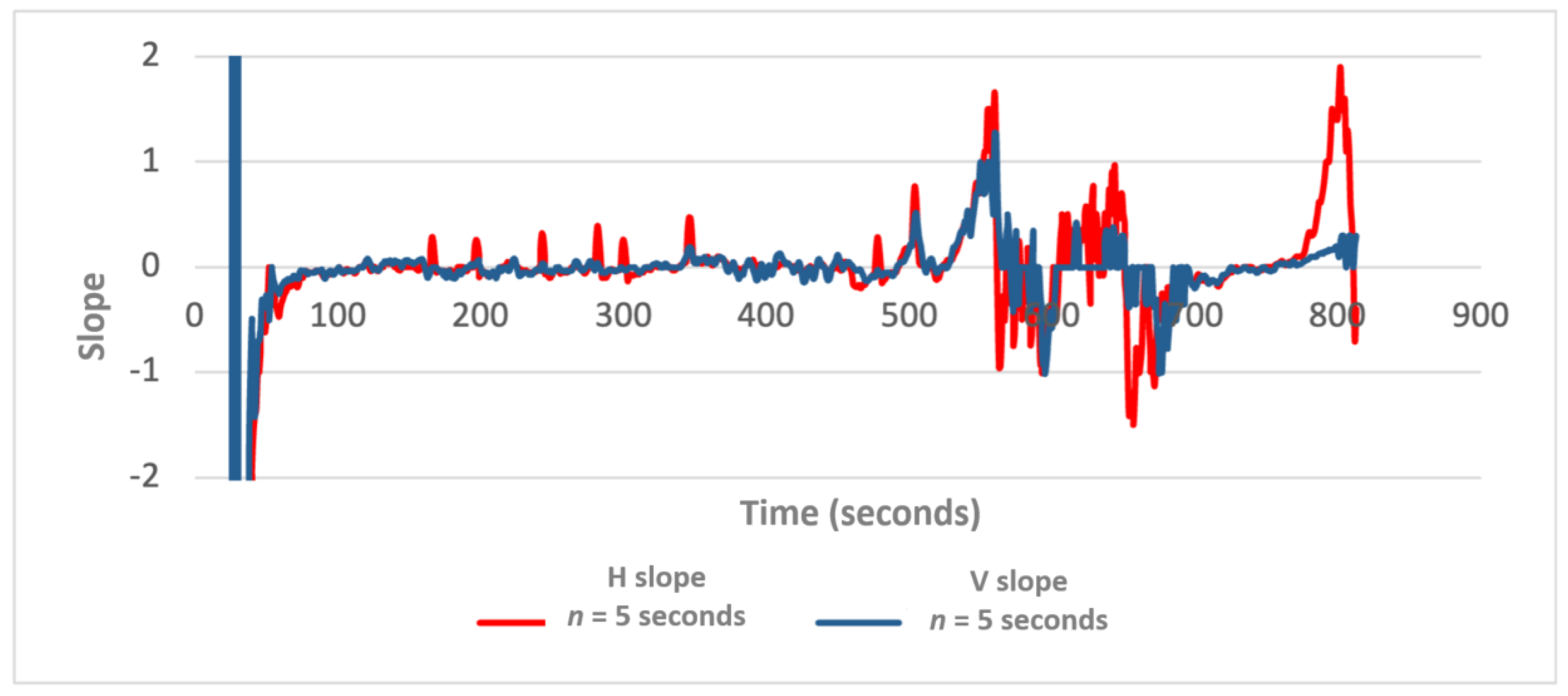
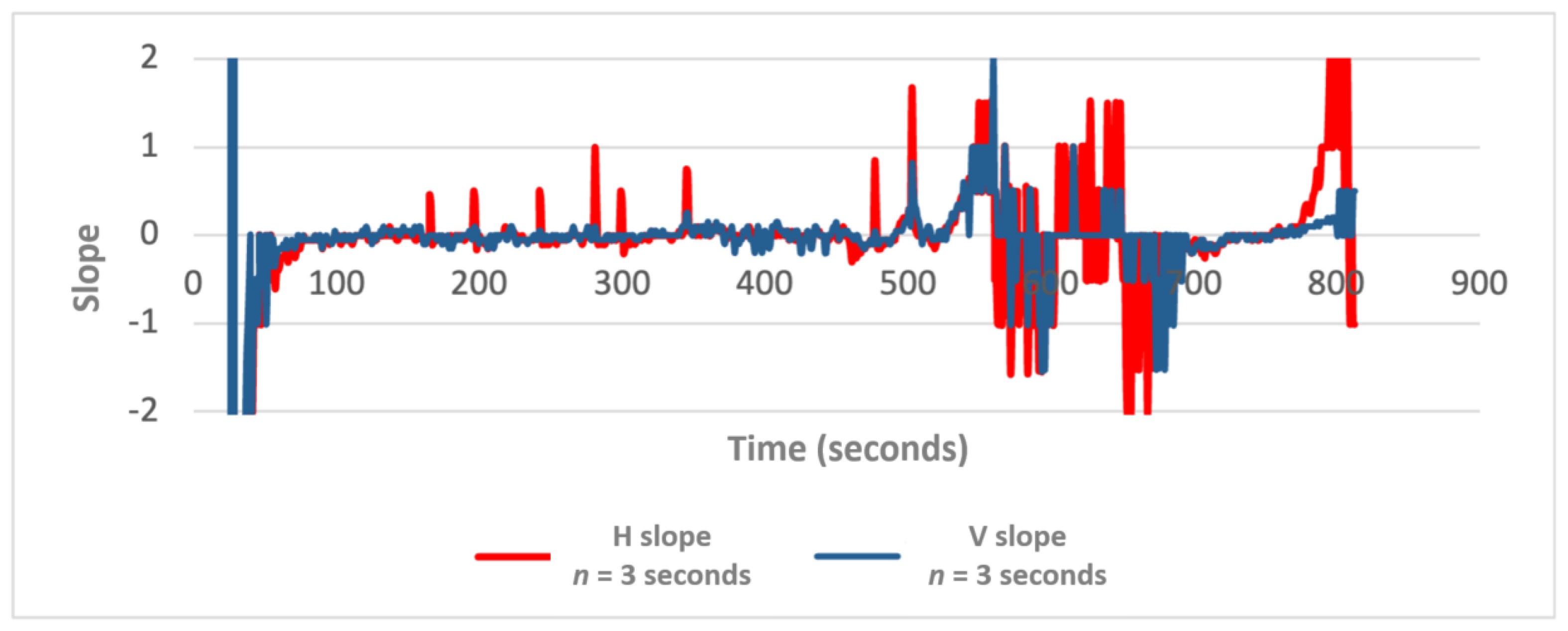
In this subsection, the slope of the horizontal error using a different time window of n = 10, 5, and 3 s has been computed and examined. The size of this window was selected due to the low motion dynamics (walking) that were used for data acquisition during tests. A very high n would imply that the positions of the people carrying out the positioning system might change significantly. The slope, defined as the ratio of the vertical change to the horizontal change between two consecutive points, when calculated over a shorter period (n = 3), highlights sharp changes in errors, while over a longer duration (n = 10), it results in a smoother representation. Figure 11, Figure 12 and Figure 13 illustrate examples of these time windows, plotting the slope derived from a set of n horizontal and vertical errors values for the “PMT-LAB” test area.

Figure 11.
Slope calculated in a time window of 10 s, using as input the horizontal error (red) and vertical error (blue).
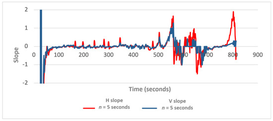
Figure 12.
Slope calculated in a time window of 5, using as input the horizontal error (red) and vertical error (blue).
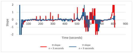
Figure 13.
Slope calculated in a time window of 3 s, using as input the horizontal error (red) and vertical error (blue).
The red peaks that emerge in each graph signify an encountered obstacle in the environment. This is promising because drastic changes are well visualized, especially in the 5- and 3-s graphs. In contrast, the graph calculated using the 10-s window does not show these peaks prominently enough (Figure 13).
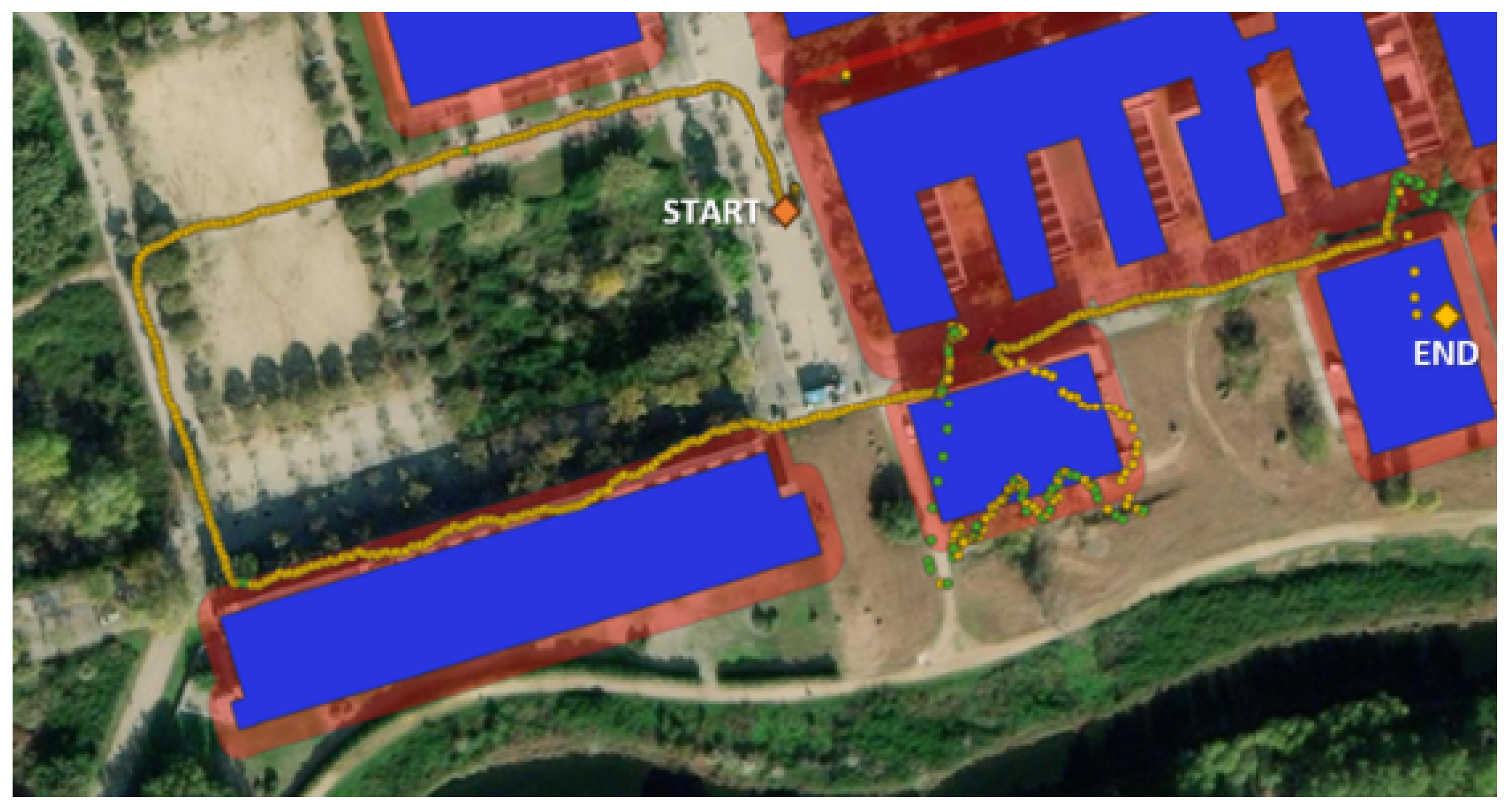
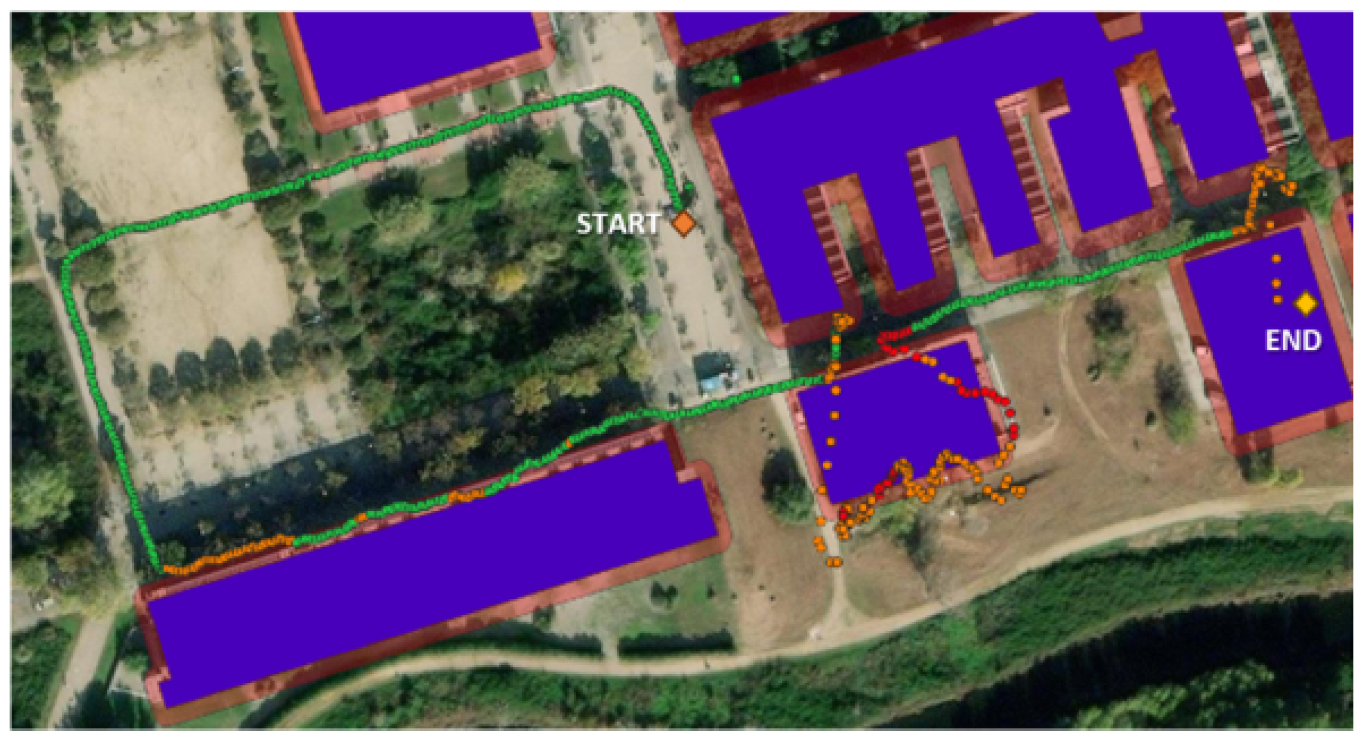
Looking for criteria to determine if the area is indoor, outdoor, or a transition area, and so to decide when the positioning system must change from GNSS-based to VIO-based trajectory solution, the slope at 3 s was chosen as an indicator as it has the sharpest peaks. Following the decision tree introduced in Figure 5, the used values are detailed thereafter: S1 = 0.5, Tin1 to a interval of [0;2] seconds; Th1 = 6 m, S2 = 1.0, Tin2 to [2;10] seconds; Th2 = 10 m, and S2 = −1.0.
Following the defined rules, they were configured in QGIS to visualise the trajectory’s appearance. The green colour denotes the moment of transition from the GNSS-based trajectory to the VIO-based trajectory, discernible near the encountered buildings. Upon analysing this outcome, it might seem suitable to switch to VIO in all the suggested cases. However, there is not a significant improvement compared to the previous results obtained from [8]. While this method might seem suitable initially, there is a notable and substantial delay, especially upon entering the last building shown in the figure below (Figure 14).

Figure 14.
Slope test applied to the trajectory of “PMT-LAB”. Yellow points are points classified as good GNSS areas, while green points are points belonging to be transition or indoor areas. Building layouts are shown in blue, while transition or semi-outdoor area for the “PMT-LAB” is shown in red.
4.4. Determination of Areas Using GNSS Mann–Kendall
Applying the MK test to the entire dataset simultaneously lacks significance. A single value computed for the entire dataset fails to discern the specific moments or locations where the trajectory is affected by the surrounding area. Furthermore, its application to small areas is unfeasible due to its requirement for real-time analysis or sequential processing of acquired data along the path. The intended approach is to employ the MK test on the most recent 10, 5, and 3 s of acquired data, with the 10-second analysis yielding the most favourable results.
At this point, we implemented a criterion similar to the one previously used for slope. While identifying the transition area remains crucial, the positioning device now switches exclusively between the GNSS-based and VIO-based trajectories. A rule distinguishing solely between outdoor and indoor areas is unnecessary; instead, we require a rule encompassing both indoor and transitional zones, which significantly impact GNSS data. Thus, we used the same criteria to detect transitional and indoor areas. The newly applied rules for this trajectory are outlined in Figure 6. The used values are detailed thereafter: S1 = 2.0, Tin1 to 10 s, Th1 = 4 m, S2 = 2.0, Tin2 to 10 s, Th2 = 4 m, S3 = −2.0, Tin3 to 10 s, and Th3 = 8 m.
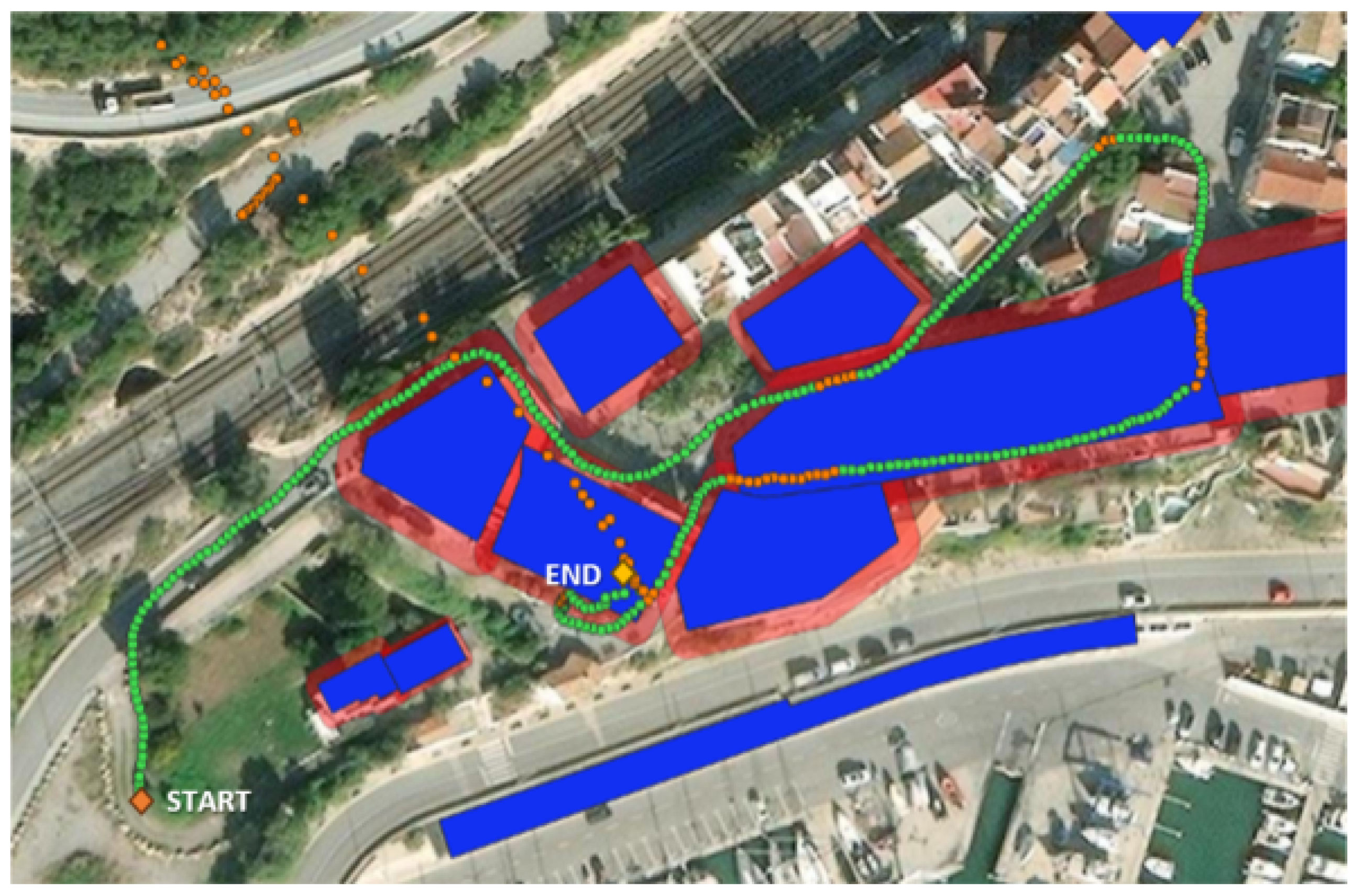
The resulting outcome is shown in a new coloured trajectory (Figure 15). The indoor area becomes recognisable before entering a building, and the outdoor area is identified in less than 10 s upon exiting indoors. Additionally, the transition areas are detected when a significant multipath affects the GNSS receiver, eliminating smaller disturbances. This improvement can significantly alter the time taken to switch from GNSS-based to VIO-based and vice versa, using only the last 10 s of collected data. Figure 16 and Figure 17 show the results of the new approach using the MK test at the Garraf, Falconera, and Collsuspina sites.
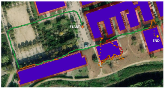
Figure 15.
MK test applied to the trajectory of “PMT-LAB”. Green points are good GNSS areas, orange points are transitional areas from outdoor to indoor, and red are from indoor to outdoor. Building layouts are shown in blue, while transition or semi-outdoor area for the “PMT-LAB” is shown in red.

Figure 16.
MK test applied to the trajectory in Garraf town. Green points are good GNSS areas, orange points are transitional areas from outdoor to indoor. Building layouts are shown in blue while transition or semi-outdoor area for the Garraf town is shown in red.
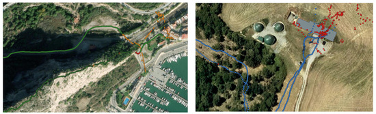
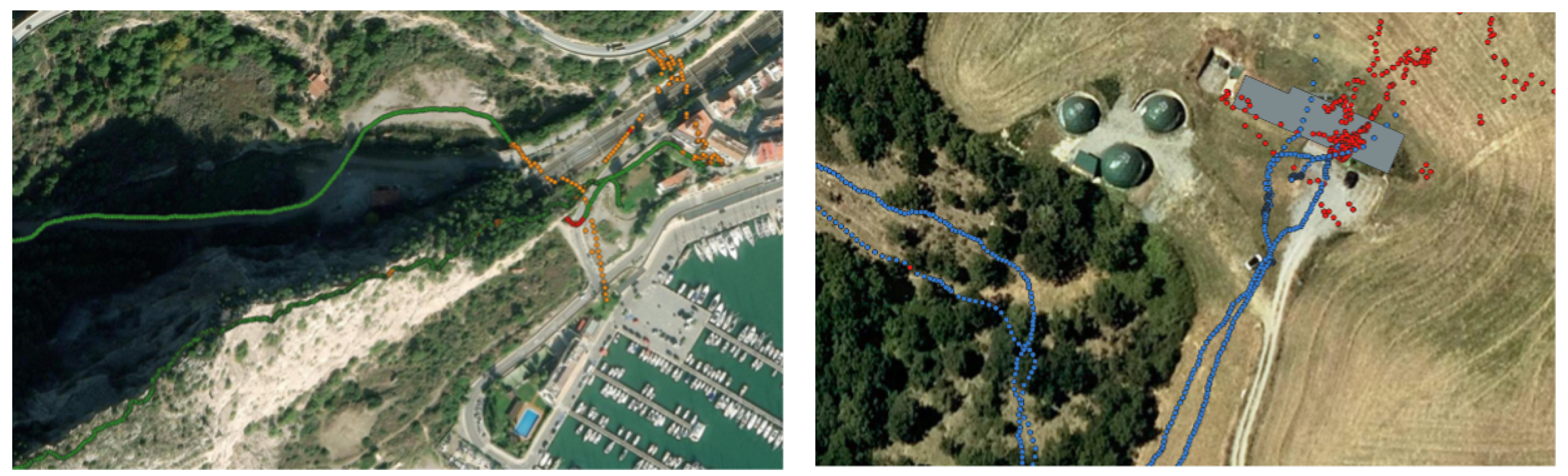
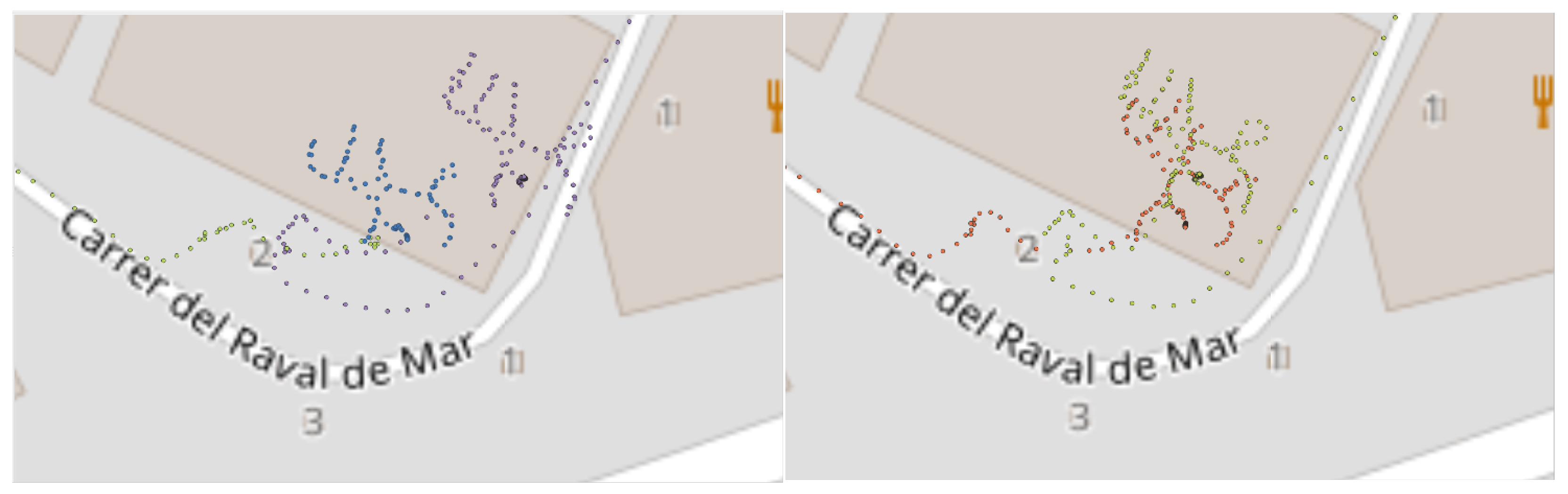
Figure 17.
MK test applied to the trajectory of Falconera (left) and Colluspina (right). On the left figure, green points are good GNSS areas, orange are transitional areas from outdoor to indoor, and red are from indoor to outdoor. On the right, blue points are good GNSS areas while red points are indoor areas.
4.5. Improved Hybrid Trajectory Using MK Context Information vs. GNSS Error Estimation Context Information
This subsection presents the results obtained with the hybrid trajectory estimation procedure.
An example of the estimated trajectory can be observed in the “PMT-LAB” case (Figure 15). Upon examining the outcomes around the second building from the bottom left, it can be observed that a user spent some time inside it. When inside a building, there might be an enhancement in the received GNSS signal as the user passes near a window, thereby entering a semi-indoor–outdoor area, for instance. Consequently, certain areas within the building might be marked as red, signifying a transition from the VIO-based to the GNSS-based solution. Nevertheless, this does not pose an operational challenge for the hybrid trajectory estimation software because transitioning from VIO-based to GNSS-based also requires waiting for the improvement of GNSS location accuracy and the classification of the area as green (outdoor).
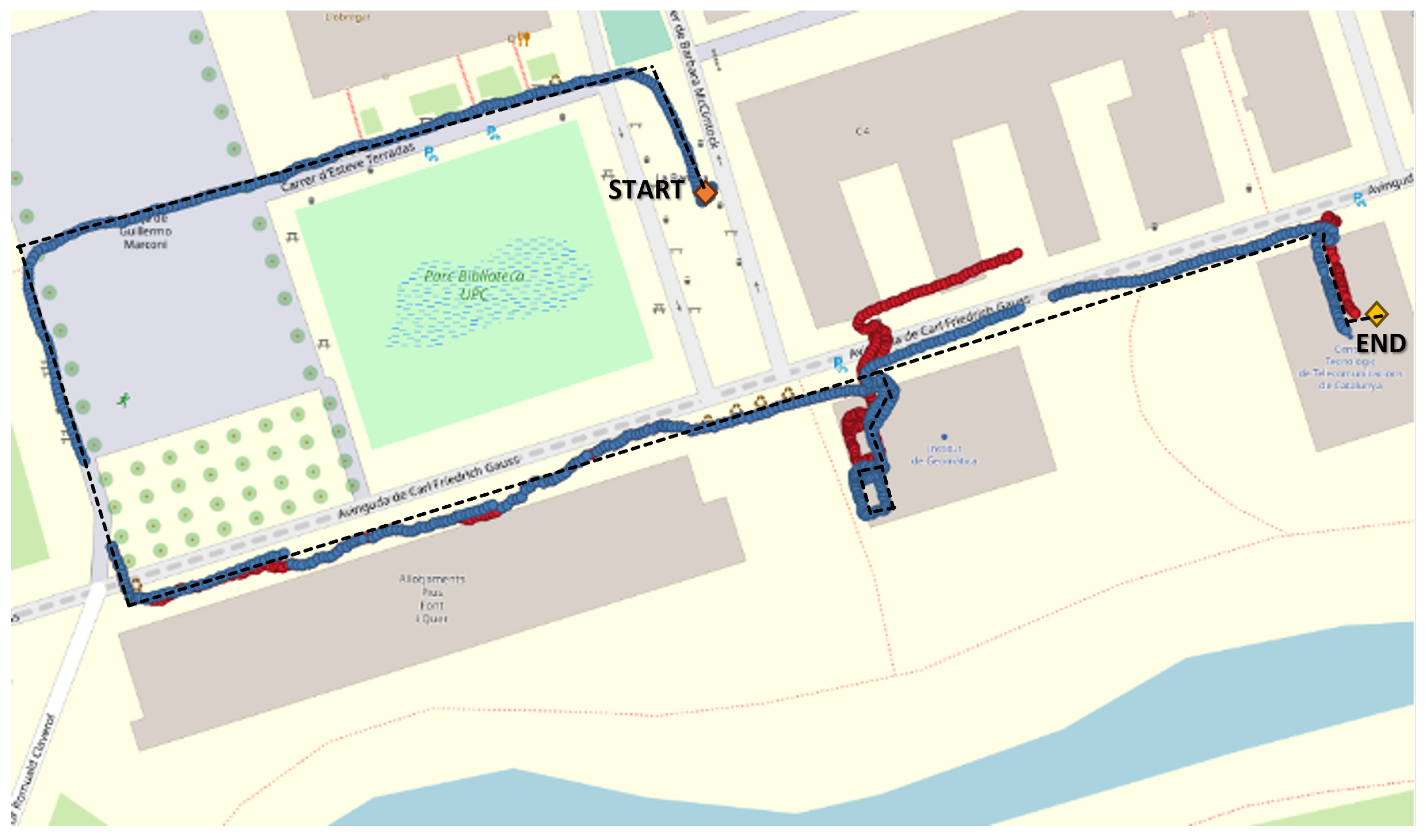
The hybrid trajectory has been estimated for the “PMT-LAB” case based on the MK outcome, as depicted in Figure 18. The newer hybrid trajectory is denoted in blue, while the older hybrid trajectory is displayed in red. Particularly noticeable within indoor spaces, the newer trajectory is much more accurate achieving less than 5 m and sub-metric precision. Furthermore, during transitions from indoors to outdoors, the updated trajectory closely mirrors the actual walking path. This similarity is especially evident in areas with GNSS open-sky conditions, such as the space between the two buildings.
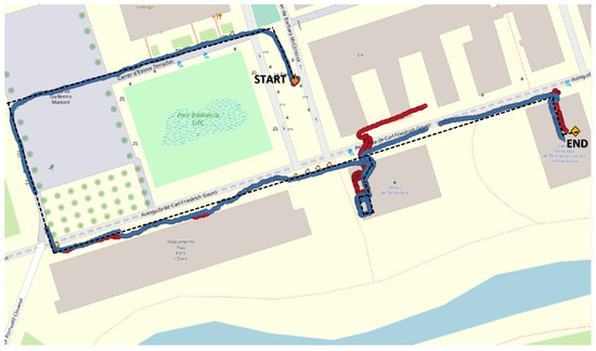
Figure 18.
Comparison of the older seamless indoor–outdoor trajectory (red) with the newer one (blue) for the “PMT-LAB”. Ground truth trajectory is depicted in black (dashed line).
The previous result highlighted the potential of this approach for urban navigation. Nevertheless, it is crucial to assess its performance across various scenarios and evaluate its reliability, especially in areas with narrow streets, dense canopy cover, or tunnels, which are integral in applications like urban mapping, logistics, and emergency management. To do so, the hybrid trajectory has been estimated for the Falconera, Garraf, and Colluspina sites, encompassing these diverse scenarios. The results are shown in Figure 19 and Figure 20.

Figure 19.
Comparison of the older (red) estimated trajectory with the newer one (blue) in Collsuspina site. Ground truth trajectory is depicted in black (dashed line).
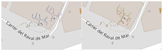
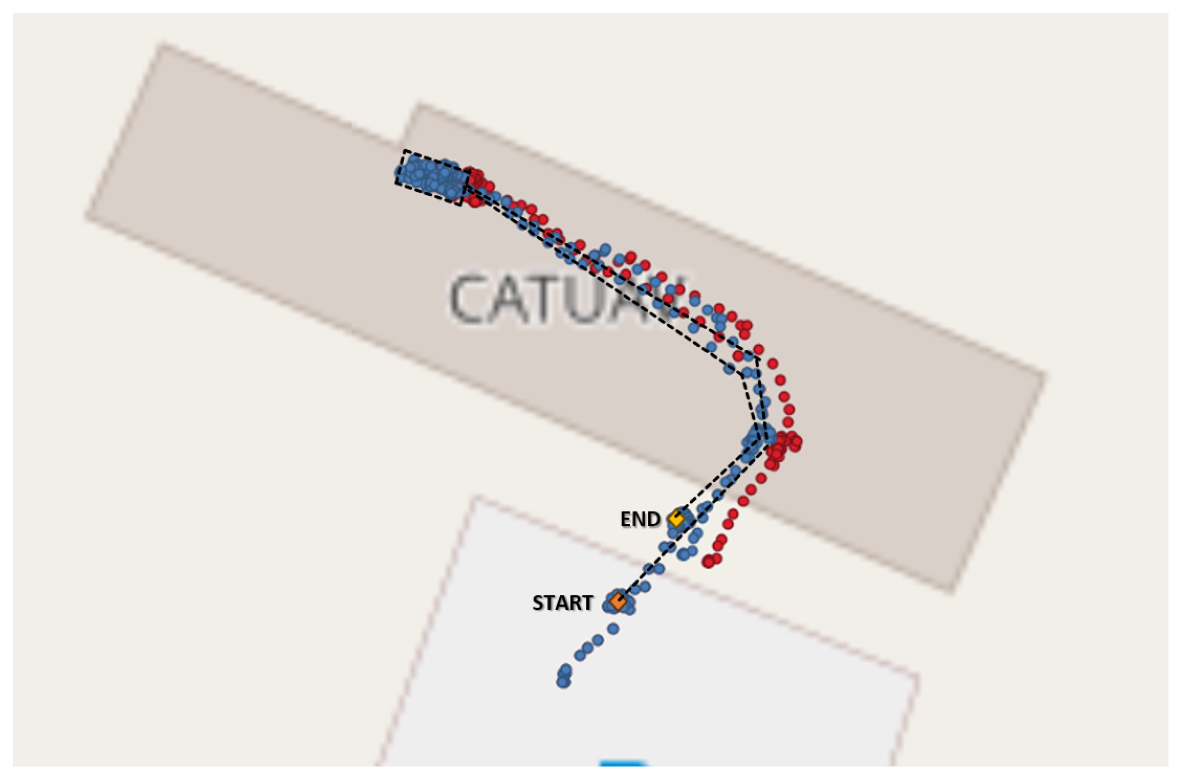
Figure 20.
The final segments of the Falconera and Garraf estimated trajectories conclude at the same building. The left side displays the previous trajectories, while the right side shows the updated trajectories.
The Collsuspina test follows a nearly symmetrical walking path, starting outdoors, moving to an inner area, and then retracing the same route back to the starting point. Figure 19 illustrates the previously estimated trajectory alongside the updated one derived from GNSS and MK test time series data. A significant deviation between the two trajectories is evident, particularly emphasising that the outbound and return paths are closer together in the blue trajectory (the new one) compared to the red one (the former trajectory). Notably, the average distance between the two trajectories has decreased from 8 to 2 m. Additionally, detailed floor plans of the building interior have been utilizsed to confirm that the updated trajectory provides greater accuracy, averaging below 5 m.
To emphasise the proposed approach more strongly, two different trajectories were estimated, each comprising distinct walking paths that concluded indoors at the same building while also following the same indoor route. These walking paths were previously illustrated in Figure 16 and Figure 17 (left image). One corresponds to the Falconera site, while the other represents the Garraf town site. As the Falconera area covered is quite extensive, the final segments of both estimated trajectories, using both the older and newer approaches, are displayed in Figure 20 below.
Given that the indoor path was identical for the conclusion of both the Falconera and Garraf trajectories, a comparison of their final segments is feasible. In Figure 20 (left), a considerable distance (averaging 10–15 m) between the two trajectories is evident when employing the older approach, based on the latest GNSS error indicator. Conversely, with the new approach (Figure 20 right), the two trajectories align closely, with an average reduction of less than 5 m. Although a slight error persists even with the new approach, it remains well within the initially established requirements.
5. Discussion and Conclusions
In this paper, we propose an enhanced approach to detecting outdoor, indoor, and transition areas based on a time series of GNSS error statistics rather than a single epoch. This approach utilises gained knowledge of the contextual environment to improve the decision strategy, for choosing between GNSS-based or VIO-based methods, thereby providing a more robust and accurate seamless indoor and outdoor trajectory. We implemented and tested two methodologies for classifying space based on a time series of GNSS error statistics. The results highlight that the method based on Mann–Kendall outperforms those based on the slope of a GNSS error time series and those based on a single epoch GNSS error statistic. The feasibility of the approach has been verified by obtaining and analysing estimated trajectories corresponding to a variety of scenarios with different characteristics. The results demonstrate that a seamless indoor–outdoor trajectory can be estimated with an accuracy below 5 m and with greater precision.
Two recent works provided a performance evaluation of estimated indoor–outdoor trajectories in scenarios with some similarities to those used in this work. In [36], the authors reported errors (in terms of 2D positioning error) of less than 15 m for the Track 6 scenario and higher than 45 m for the Track 3 scenario. Meanwhile, in [37], the authors reported errors for the Door01 (indoor–outdoor switching) scenario between 0.7 and 9.3 m using VIO-based approaches or GNSS-RTK based approaches. Although these scenarios are similar to those presented in the results section, a quantitative evaluation cannot be properly performed since the scenarios, positioning sensors, and motion dynamics are not the same. Future work should include the additional validation of our approach using other scenarios/datasets, including other motion dynamics (robot and car), and a comparison of the performance achieved with the proposed approach against other state-of-the-art approaches using benchmark datasets such as WHUVID [38] and M2DGR [37].
While this work represents a step forward in seamless indoor–outdoor positioning performance, there is still room for improvement in terms of overall performance and robustness. Consideration of context information is essential to enhance the fusion strategy in future works and to characterise the features of these transition areas. Implementing the semantic classification of urban scenes and scene/place recognition using images provided by the VIO system and deep learning techniques, as proposed in studies such as those by [39,40,41,42], could be beneficial. Furthermore, considering hybrid methods that merge the current approach with a trajectory forecasting approach based on Artificial Intelligence, as suggested in works by [43,44], could also be valuable.
The research presented here originates from the IOPES project, which aimed to continuously and robustly track members of civil protection or emergency teams, regardless of whether they are indoors or outdoors, during the emergency or post-emergency phase of a disaster [13]. The proposed solution operates independently of any deployed infrastructure, yet it is delivered through cost-effective equipment, intending to serve a wide number of users. This dual combination may enable the adoption of the proposed solution by other groups that might need robust and continuously seamless indoor/outdoor positioning, such as elderly and differently-abled people [1], wildlife [45], or warehouse assets [21]. Moreover, the proposed solution holds potential for applications in autonomous car and robot navigation; various automotive services such as vehicle accident detection; smart parking systems; and the estimation of free slots, real-time car parking monitoring, and automatic billing [21]. Furthermore, it could be combined with mapping sensors to generate point clouds that can be used with further post-processing for building information modeling purposes or virtual reality applications.
Author Contributions
Conceptualization, Alban Gorreja, Eduard Angelats, Roberto Pierdicca, and Eva Savina Malinverni; methodology, Alban Gorreja, Eduard Angelats and M. Eulàlia Parés; software, Alban Gorreja and Eduard Angelats; validation, Alban Gorreja and Eduard Angelats; formal analysis, Alban Gorreja and Eduard Angelats; investigation, Alban Gorreja, Eduard Angelats, M. Eulàlia Parés, Roberto Pierdicca and Eva Savina Malinverni; resources, Roberto Pierdicca and Eva Savina Malinverni; data curation, Pedro F. Espín-López; writing—original draft preparation, Alban Gorreja, Eduard Angelats, M. Eulàlia Parés and Roberto Pierdicca; writing—review and editing, Alban Gorreja, Eduard Angelats, M. Eulàlia Parés, Pedro F. Espín-López, Roberto Pierdicca and Eva Savina Malinverni; visualization, Alban Gorreja; supervision, Roberto Pierdicca and Eva Savina Malinverni; project administration, Roberto Pierdicca and Eva Savina Malinverni; and funding acquisition, Alban Gorreja, Roberto Pierdicca and Eva Savina Malinverni. All authors have read and agreed to the published version of the manuscript.
Funding
The data used in this research were acquired in the frame of the IOPES project funded from the European Commission, Directorate-General Humanitarian Aid and Civil Protection (ECHO), under the call UCPM-2019-PP-AG. E.A, M.E.P, and P.E received funds from Generalitat de Catalunya through 2021SGR00536 grant.
Data Availability Statement
Data are available on request to the authors.
Conflicts of Interest
The authors declare no conflicts of interest.
Abbreviations
The following abbreviations are used in this manuscript:
| GNSS | Global Navigation Satellite System |
| H_err | Horizontal error |
| IMU | Inertial Measurement Unit |
| MK | Mann–Kendall |
| NLOS | Non Line of Sight |
| RGB-D | Red Green Blue-Depth |
| S | Slope |
| S_i | Slope number i |
| SLAM | Simultaneous localization and mapping |
| UWB | Ultra-Wide Band |
| Th | Threshold |
| Th i | Threshold number i |
| T_in | Time to get in/out to/from indoor |
| T_in i | Time to get in/out to/from indoor number i |
| V_err | Vertical Error |
| VIO | Visual Inertial Odometry |
Appendix A
The following assumptions underlie the MK test (https://vsp.pnnl.gov/help/index.htm#vsample/design_trend_mann_kendall.htm (accessed on 1 February 2024)):
- When no trend is present, the measurements (observations or data) obtained over time are independent and identically distributed. The assumption of independence means that the observations are not serially correlated over time.
- The observations obtained over time are representative of the true conditions at sampling times.
- The sample collection, handling, and measurement methods provide unbiased and representative observations of the underlying populations over time.
The mean of S is , and the variance is
where p is the number of the tied groups in the data set and is the number of data points in the tied group. The statistic S is approximately normal distributed provided that the following Z-transformation is employed:
References
- Mallik, M.; Panja, A.K.; Chowdhury, C. Paving the way with machine learning for seamless indoor–outdoor positioning: A survey. Inf. Fusion 2023, 94, 126–151. [Google Scholar] [CrossRef]
- Rossi, L.; Ajmar, A.; Paolanti, M.; Pierdicca, R. Vehicle trajectory prediction and generation using LSTM models and GANs. PLoS ONE 2021, 16, e0253868. [Google Scholar] [CrossRef] [PubMed]
- Osaba, E.; Pierdicca, R.; Malinverni, E.S.; Khromova, A.; Álvarez, F.J.; Bahillo, A. A smartphone-based system for outdoor data gathering using a wireless beacon network and GPS data: From cyber spaces to senseable spaces. ISPRS Int. J.-Geo-Inf. 2018, 7, 190. [Google Scholar] [CrossRef]
- Cheng, T.; Teizer, J. Real-time resource location data collection and visualization technology for construction safety and activity monitoring applications. Autom. Constr. 2013, 34, 3–15. [Google Scholar] [CrossRef]
- Mautz, R. Overview of current indoor positioning systems. Geod. Kartogr. 2009, 35, 18–22. [Google Scholar] [CrossRef]
- Ho, H.Y.; Ng, H.F.; Leung, Y.T.; Wen, W.; Hsu, L.T.; Luo, Y. Smartphone level indoor/outdoor ubiquitous pedestrian positioning 3DGMA GNSS/VINS integration using FGO. Int. Arch. Photogramm. Remote Sens. Spat. Inf. Sci. 2023, 48, 175–182. [Google Scholar] [CrossRef]
- Bai, Y.B.; Holden, L.; Kealy, A.; Zaminpardaz, S.; Choy, S. A hybrid indoor/outdoor detection approach for smartphone-based seamless positioning. J. Navig. 2022, 75, 946–965. [Google Scholar] [CrossRef]
- Angelats, E.; Espín-López, P.; Navarro, J.; Parés, M. Performance analysis of the iopes seamless indoor–outdoor positioning approach. Int. Arch. Photogramm. Remote Sens. Spat. Inf. Sci. 2021, 43, 229–235. [Google Scholar] [CrossRef]
- Cioffi, G.; Scaramuzza, D. Tightly-coupled Fusion of Global Positional Measurements in Optimization-based Visual-Inertial Odometry. In Proceedings of the 2020 IEEE/RSJ International Conference on Intelligent Robots and Systems (IROS), Las Vegas, NV, USA, 25–29 October 2020; pp. 5089–5095. [Google Scholar] [CrossRef]
- Lee, W.; Geneva, P.; Yang, Y.; Huang, G. Tightly-coupled GNSS-aided Visual-Inertial Localization. In Proceedings of the 2022 International Conference on Robotics and Automation (ICRA), Philadelphia, PA, USA, 23–27 May 2022; pp. 9484–9491. [Google Scholar] [CrossRef]
- Boche, S.; Zuo, X.; Schaefer, S.; Leutenegger, S. Visual-Inertial SLAM with Tightly-Coupled Dropout-Tolerant GPS Fusion. In Proceedings of the 2022 IEEE/RSJ International Conference on Intelligent Robots and Systems (IROS), Kyoto, Japan, 23–27 October 2022; pp. 7020–7027. [Google Scholar] [CrossRef]
- Cao, S.; Lu, X.; Shen, S. GVINS: Tightly Coupled GNSS–Visual–Inertial Fusion for Smooth and Consistent State Estimation. IEEE Trans. Robot. 2022, 38, 2004–2021. [Google Scholar] [CrossRef]
- Parés, M.; Angelats, E.; Espín-López, P.; Navarro, J.; Munaretto, D.; Salvador, J.; Delgado, C.; Olbrich, F.; Martínez, A.; Örn Arnarson, G.; et al. IOPES, a new full-fledged approach to provide an end-to-end tracking system for emergency staff. Int. J. Disaster Risk Reduct. 2024, 100, 104180. [Google Scholar] [CrossRef]
- Angelats., E.; Navarro, J.A.; Parés Calaf, M.E. Towards seamless indoor–outdoor positioning: The IOPES project approach. In Proceedings of the International Archives of the Photogrammetry, Remote Sensing and Spatial Information Sciences: XXIV ISPRS Congress, Commission IV (Volume XLIII-B4-2020), Online, 22–26 June 2020; pp. 313–319. [Google Scholar] [CrossRef]
- Alinsavath, K.N.; Nugroho, L.E.; Widyawan; Hamamoto, K. The seamlessness of outdoor and indoor localization approaches based on a ubiquitous computing environment: A survey. In Proceedings of the 2nd International Conference on Information Science and Systems, Tokyo, Japan, 16–19 March 2019; pp. 316–324. [Google Scholar] [CrossRef]
- Chumkamon, S.; Tuvaphanthaphiphat, P.; Keeratiwintakorn, P. A blind navigation system using RFID for indoor environments. In Proceedings of the 2008 5th International Conference on Electrical Engineering/Electronics, Computer, Telecommunications and Information Technology, Krabi, Thailand, 14–17 May 2008; Volume 2, pp. 765–768. [Google Scholar] [CrossRef]
- Jiang, W.; Cao, Z.; Cai, B.; Li, B.; Wang, J. Indoor and outdoor seamless positioning method using UWB enhanced multi-sensor tightly-coupled integration. IEEE Trans. Veh. Technol. 2021, 70, 10633–10645. [Google Scholar] [CrossRef]
- Sturari, M.; Liciotti, D.; Pierdicca, R.; Frontoni, E.; Mancini, A.; Contigiani, M.; Zingaretti, P. Robust and affordable retail customer profiling by vision and radio beacon sensor fusion. Pattern Recognit. Lett. 2016, 81, 30–40. [Google Scholar] [CrossRef]
- Saeed, N.; Nam, H.; Al-Naffouri, T.Y.; Alouini, M.S. A state-of-the-art survey on multidimensional scaling-based localization techniques. IEEE Commun. Surv. Tutor. 2019, 21, 3565–3583. [Google Scholar] [CrossRef]
- Maghdid, H.S.; Lami, I.A.; Ghafoor, K.Z.; Lloret, J. Seamless outdoors-indoors localization solutions on smartphones: Implementation and challenges. ACM Computing Surv. CSUR 2016, 48, 1–34. [Google Scholar] [CrossRef]
- Asaad, S.M.; Maghdid, H.S. A comprehensive review of indoor/outdoor localization solutions in IoT era: Research challenges and future perspectives. Comput. Netw. 2022, 212, 109041. [Google Scholar] [CrossRef]
- Zlatanova, S.; Yan, J.; Wang, Y.; Diakité, A.; Isikdag, U.; Sithole, G.; Barton, J. Spaces in spatial science and urban applications—state of the art review. ISPRS Int. J.-Geo-Inf. 2020, 9, 58. [Google Scholar] [CrossRef]
- Xie, P.; Petovello, M.G. Measuring GNSS multipath distributions in urban canyon environments. IEEE Trans. Instrum. Meas. 2014, 64, 366–377. [Google Scholar]
- Næsset, E.; Gjevestad, J.G. Performance of GPS precise point positioning under conifer forest canopies. Photogramm. Eng. Remote Sens. 2008, 74, 661–668. [Google Scholar] [CrossRef]
- Zlatanova, S.; Liu, L.; Sithole, G. A conceptual framework of space subdivision for indoor navigation. In Proceedings of the Fifth ACM SIGSPATIAL International Workshop on Indoor Spatial Awareness, Orlando, FL, USA, 5 November 2013; pp. 37–41. [Google Scholar] [CrossRef]
- Zlatanova, S.; Liu, L.; Sithole, G.; Zhao, J.; Mortari, F. Space Subdivision for Indoor Applications; Delft University of Technology, OTB Research Institute for the Built Environment: Delft, The Netherlands, 2014. [Google Scholar] [CrossRef]
- Yang, L.; Worboys, M. Similarities and differences between outdoor and indoor space from the perspective of navigation. In Proceedings of the Conference on Spatial Information Theory (COSIT 2011), Belfast, ME, USA, 12–16 September 2011. [Google Scholar]
- Yang, Z.; Wu, C.; Liu, Y. Locating in fingerprint space: Wireless indoor localization with little human intervention. In Proceedings of the 18th Annual International Conference on Mobile Computing and Networking, Istanbul, Turkey, 22–26 August 2012; pp. 269–280. [Google Scholar] [CrossRef]
- Kray, C.; Fritze, H.; Fechner, T.; Schwering, A.; Li, R.; Anacta, V.J. Transitional spaces: Between indoor and outdoor spaces. In Proceedings of the Spatial Information Theory: 11th International Conference, COSIT 2013, Scarborough, UK, 2–6 September 2013; Proceedings 11. Springer: Berlin/Heidelberg, Germany, 2013; pp. 14–32. [Google Scholar] [CrossRef]
- Ortiz, A.; Bonnin-Pascual, F.; Garcia-Fidalgo, E.; Company, J.P. Saliency-driven Visual Inspection of Vessels by means of a Multirotor. In Proceedings of the Workshop on Vision-Based Control & Navigation of Small Lightweight UAVs, Hamburg, Germany, 28 September–2 October 2015; pp. 20–46. [Google Scholar]
- Wang, W.; Chang, Q.; Li, Q.; Shi, Z.; Chen, W. indoor–outdoor detection using a smart phone sensor. Sensors 2016, 16, 1563. [Google Scholar] [CrossRef] [PubMed]
- Feriol, F.; Vivet, D.; Watanabe, Y. A review of environmental context detection for navigation based on multiple sensors. Sensors 2020, 20, 4532. [Google Scholar] [CrossRef] [PubMed]
- Kendall, M.G. Rank correlation methods. J. Inst. Actuar. 1948, 75, 140–141. [Google Scholar] [CrossRef]
- Mann, H.B. Nonparametric tests against trend. Econom. J. Econom. Soc. 1945, 13, 245–259. [Google Scholar] [CrossRef]
- Yue, S.; Pilon, P.; Cavadias, G. Power of the Mann–Kendall and Spearman’s rho tests for detecting monotonic trends in hydrological series. J. Hydrol. 2002, 259, 254–271. [Google Scholar] [CrossRef]
- Potortì, F.; Crivello, A.; Lee, S.; Vladimirov, B.; Park, S.; Chen, Y.; Wang, L.; Chen, R.; Zhao, F.; Zhuge, Y.; et al. Offsite evaluation of localization systems: Criteria, systems and results from IPIN 2021-22 competitions. IEEE J. Indoor Seamless Position. Navig. 2024, 1–39. [Google Scholar] [CrossRef]
- Yin, J.; Li, A.; Li, T.; Yu, W.; Zou, D. M2DGR: A Multi-sensor and Multi-scenario SLAM Dataset for Ground Robots. IEEE Robot. Autom. Lett. 2021, 7, 2266–2273. [Google Scholar] [CrossRef]
- Chen, T.; Pu, F.; Chen, H.; Liu, Z. WHUVID: A Large-Scale Stereo-IMU Dataset for Visual-Inertial Odometry and Autonomous Driving in Chinese Urban Scenarios. Remote Sens. 2022, 14, 2033. [Google Scholar] [CrossRef]
- López-Cifuentes, A.; Escudero-Viñolo, M.; Bescós, J.; García-Martín, Á. Semantic-aware scene recognition. Pattern Recognit. 2020, 102, 107256. [Google Scholar] [CrossRef]
- Zhang, X.; Wang, L.; Su, Y. Visual place recognition: A survey from deep learning perspective. Pattern Recognit. 2021, 113, 107760. [Google Scholar] [CrossRef]
- Yang, M.Y.; Kumaar, S.; Lyu, Y.; Nex, F. Real-time semantic segmentation with context aggregation network. ISPRS J. Photogramm. Remote Sens. 2021, 178, 124–134. [Google Scholar] [CrossRef]
- Xie, Y.; Yan, J.; Kang, L.; Guo, Y.; Zhang, J.; Luan, X. FCT: Fusing CNN and transformer for scene classification. Int. J. Multimed. Info. Retr. 2022, 11, 611–618. [Google Scholar] [CrossRef]
- Gupta, A.; Johnson, J.; Fei-Fei, L.; Savarese, S.; Alahi, A. Social GAN: Socially Acceptable Trajectories with Generative Adversarial Networks. In Proceedings of the 2018 IEEE/CVF Conference on Computer Vision and Pattern Recognition, Salt Lake City, UT, USA, 18–23 June 2018; pp. 2255–2264. [Google Scholar] [CrossRef]
- Rossi, L.; Paolanti, M.; Pierdicca, R.; Frontoni, E. Human trajectory prediction and generation using LSTM models and GANs. Pattern Recognit. 2021, 120, 108136. [Google Scholar] [CrossRef]
- Tenreiro Machado, J.; Lopes, A.M. Analysis of forest fires by means of pseudo phase plane and multidimensional scaling methods. Math. Probl. Eng. 2014, 2014, 575872. [Google Scholar] [CrossRef]

Disclaimer/Publisher’s Note: The statements, opinions and data contained in all publications are solely those of the individual author(s) and contributor(s) and not of MDPI and/or the editor(s). MDPI and/or the editor(s) disclaim responsibility for any injury to people or property resulting from any ideas, methods, instructions or products referred to in the content. |
© 2024 by the authors. Licensee MDPI, Basel, Switzerland. This article is an open access article distributed under the terms and conditions of the Creative Commons Attribution (CC BY) license (https://creativecommons.org/licenses/by/4.0/).