Abstract
The Voronoi diagram on the Earth’s surface is a significant data model, characterized by natural proximity and dynamic stability, which has emerged as one of the most promising solutions for global spatial dynamic management and analysis. However, traditional algorithms for generating spherical raster Voronoi diagrams find it challenging to dynamically adjust the Voronoi diagram while maintaining precision and efficiency. The efficient and accurate construction of the spherical Voronoi diagram has become one of the bottleneck issues limiting its further large-scale application. To this end, this paper proposes a dynamic construction scheme for the spherical Voronoi diagram based on the QTM (Quaternary Triangular Mesh) system, with the aim of enabling efficient generation, local updates, and multi-scale visualization of the spherical Voronoi diagrams. In this paper, canonical ordering is introduced. Tailored for the properties of the spherical triangular grid, it constructs a unified and standardized sorting strategy for the dilation of the spherical grids. The construction and updating of the spherical Voronoi diagram are achieved through the ordered dilation of sites. Furthermore, the multi-scale visualization of the spherical Voronoi diagram is realized through the hierarchical structure of the QTM. The paper presents our algorithm intuitively through pseudocode, conducts comparative experiments on the feasibility and efficiency, and designs an experiment for the dynamic navigation and management of ocean-going vessels based on the global multi-resolution Voronoi diagram. The experimental results demonstrate that our algorithm effectively controls the error of the generation of the raster Voronoi diagram and has a significant efficiency advantage when processing dynamic environments.
1. Introduction
With the rapid advancement of space science and technology, coupled with the continuous deepening of global economic integration, the scope of human research has progressively expanded from localized regions to encompass the entire globe. The evolution of modern surveying techniques, including photogrammetry, remote sensing, and GPS, has enabled the acquisition of extensive, multi-scale, and multi-temporal data on a global scale. To effectively store, manage, and analyze spatial data across the globe, there is a necessity for the development of a global, continuous, and multi-scale dynamic data model. Spherical Voronoi diagrams, as a significant data model endowed with beneficial attributes such as natural proximity and dynamic stability, have been widely utilized in critical domains including oceanography, meteorology, airspace management, and satellite planning [1,2,3,4,5]. They stand out as one of the most promising approaches for the dynamic management and analysis of global spatial information.
Existing algorithms for generating spherical Voronoi diagrams are often extensions of their planar counterparts. They can be categorized based on the foundational models they employ: algorithms based on vector models and those based on raster models. Both categories of algorithms possesses distinct characteristics, making them suitable for a variety of applications.
Vector algorithms [6,7,8,9,10,11] generally perform well with sets of points on the sphere, but they encounter complex calculations and produce intricate data structures when dealing with sets of lines and surfaces on the sphere. Moreover, the results of vector algorithms are not conducive to the multi-scale representation of spatial data. Additionally, constructing vector Voronoi diagrams on an ellipsoidal surface requires iterative calculations based on approximate coordinates of an auxiliary sphere [2]. The vector Voronoi diagrams struggle to fundamentally address the challenges of multi-scale integrated processing and the comprehensive analysis of massive global data [12], which is one of the bottleneck issues limiting their wider application on a larger scale.
In Earth science applications, the generation of Voronoi diagrams based on raster models is of significant importance. First, raster Voronoi diagrams allow for the multi-scale visualization of complex shapes through a set of grids, reducing the complexity associated with constructing Voronoi diagrams for spherical line and surface sets and simplifying the generation process for these geometric elements. Second, the algorithms for generating these diagrams are more easily extended to ellipsoidal surfaces, eliminating the need for additional computational steps. Lastly, grids are pivotal within the digital Earth system, serving as the foundational structure for contemporary digital and intelligent management applications [13]. A wide variety of data, including remote sensing imagery, are stored and represented in raster format. Raster-based Voronoi diagrams utilize this grid data directly, thus avoiding the complex conversion process from raster to vector formats [14].
Many scholars have conducted research on the generation of raster-based spherical Voronoi diagrams. In 2003, Zhao et al. [12] proposed a classic dilation algorithm for constructing spherical raster Voronoi diagrams, which partitions the sphere into a Quaternary Triangular Mesh (QTM) grid and then uses dilation from digital morphology to progressively expand generation points throughout the sphere. However, utilizing the QTM grid distance as the benchmark for dilation results in an approximation of the exact Voronoi diagram on Earth, with errors that are challenging to control [14]. Furthermore, the dilation process necessitates the manipulation of all neighboring grids, including the repeated selection and subsequent elimination of duplicates, which introduces significant computational overhead and substantially reduces algorithmic efficiency. In 2014, Hu et al. [14] introduced an ellipsoid-based raster Voronoi diagram generation algorithm that employs an ellipsoidal distance metric during the raster scan distance transformation process. In 2022, Kazemi et al. [15] leveraged the multi-resolution properties of Discrete Global Grid Systems, employing a hierarchical and progressive approach to implement an efficient spherical distance transformation algorithm. The algorithms developed by Hu and Kazemi significantly improved the construction efficiency of raster Voronoi diagrams and were effective in controlling errors within the confines of a single grid.
However, the algorithms by Hu and Kazemi encounter significant challenges in dynamically constructing Voronoi diagrams. In the myriad of practical applications for Voronoi diagrams, the underlying environments frequently experience dynamic changes. These changes necessitate real-time updates and ongoing maintenance to ensure the accuracy and effectiveness of the Voronoi diagram. Given the dynamic stability characteristic of Voronoi diagrams, only the parts corresponding to the local regions affected by environmental changes undergo alteration, while the majority of the overall diagram’s structure remains unaffected. Utilizing its local mechanism, this targeted process, which addresses changes solely within the affected Voronoi regions and precludes the need for a comprehensive reconstruction of the entire diagram, is referred to as a Voronoi diagram update. In most instances, this approach can significantly reduce computational costs. The algorithm by Hu and Kazemi does not possess a strategy capable of accurately pinpointing the regions that necessitate updates, thereby rendering it unsuitable for direct application in Voronoi diagram updates. As illustrated in Figure 1, Figure 1a depicts the Voronoi diagram constructed with generation points A, B, C, and D. Upon the insertion of a new generation point E within the Voronoi region of point D, the resulting updated Voronoi diagram is shown in Figure 1b. The gray area in this figure represents the Voronoi region corresponding to the new generation point E and is also the region where the Voronoi diagram has undergone change. It can be observed from Figure 1b that this area overlaps with parts of the Voronoi regions originally associated with generation points A, B, C, and D. This region is neither enclosed by the region formed by the neighboring generation points of point D nor covered by the Voronoi regions corresponding to the neighboring generation points of point D. Consequently, it is not feasible to determine the area needing an update based solely on the topological adjacency of the inserted point.
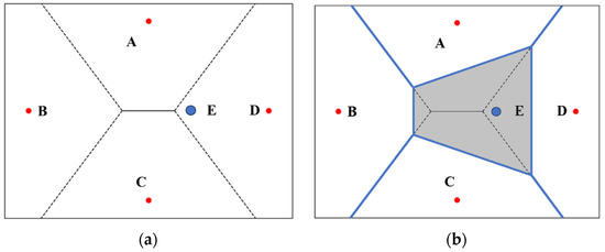
Figure 1.
The update area in the Voronoi diagram. (a) Voronoi diagram with generation points A, B, C, and D. (b) Updated diagram with generation points A, B, C, D and E.
Canonical ordering, a strategy for the rearrangement of matrices, is utilized to reorganize complex topological structures into a simplified, ordered list or sequence. This method reduces the complexity of processing, facilitating more convenient analysis and visualization. It has been widely applied in various fields, including optimized image processing, real-time pathfinding on regular grids, and distance transformations on planar lattices [16,17,18,19]. However, due to significant topological differences between spherical and planar spaces, and considering the singularities at the Earth’s poles and the distortions caused by projection [15], the rules of canonical ordering applicable to planar lattices are not directly transferable to spherical spaces.
This paper introduces a canonical ordering strategy and presents a dynamic construction scheme for spherical Voronoi diagrams based on the Quaternary Triangular Mesh (QTM) system. This scheme is tailored for the generation, dynamic updating, and multi-scale visualization of spherical Voronoi diagrams. Initially, the Earth’s surface is partitioned according to the QTM methodology. Subsequently, a three-level data structure, composed of dictionaries and queues, is designed. Thereafter, an ordered dilation algorithm is devised. By incorporating the canonical ordering strategy and considering the properties of the spherical triangular grid, a procedural sequence for the ordered dilation of the spherical grids is designed. Special treatment methods are also developed to address changes in the topological structure of neighborhoods across the basic faces. A unified and standardized sorting framework is constructed for the grid dilation process, aiming to enhance overall efficiency and performance. Ultimately, the spherical Voronoi diagram is constructed and updated through the ordered dilation of points, lines, and surfaces on the sphere. The delineation of the update region’s boundary is determined by the grid dilation. Additionally, the multi-resolution attribute of the grid enables the multi-scale visualization of the global Voronoi diagram.
This paper is organized into five sections, beginning with an introduction. Section 2 details the specific steps of the ordered dilation algorithm proposed for the generation and rapid local updating of spherical Voronoi diagrams. Section 3 presents a comparative analysis of the algorithm’s feasibility and efficiency, complemented by an application demonstration. Section 4 offers discussions on the findings. Section 5 concludes the paper.
2. Methods
2.1. Selection of the Base Model
The Discrete Global Grid System (DGGS) serves as a foundational model for the modern digital Earth framework, based on real geospatial space. It conforms to the Earth’s surface through infinite recursive subdivision of the sphere, thereby avoiding the distortions and data gaps inherent in planar projections. Utilizing grid coding in place of traditional geographic coordinates for data manipulation, the DGGS establishes a seamless and non-overlapping multi-resolution grid hierarchy. This system facilitates the effective integration, organization, and management of globally sourced, multi-scale foundational data, functioning as a platform for the integration and sharing of heterogeneous spatial data. The DGGS has been widely applied in various fields [20,21,22,23,24].
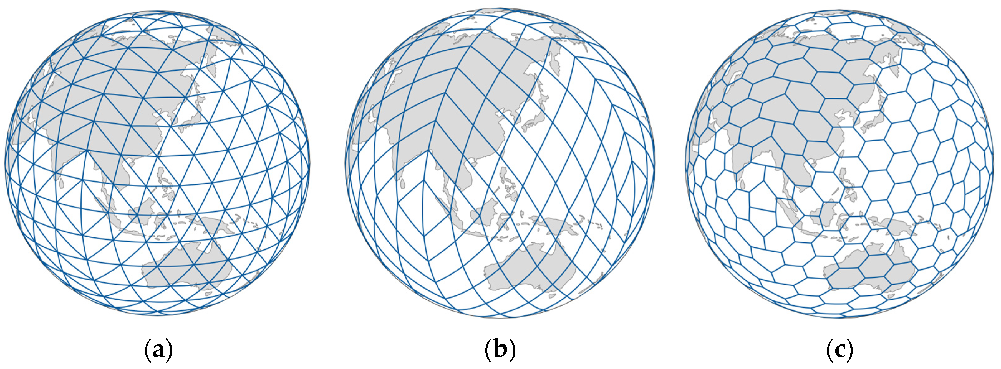
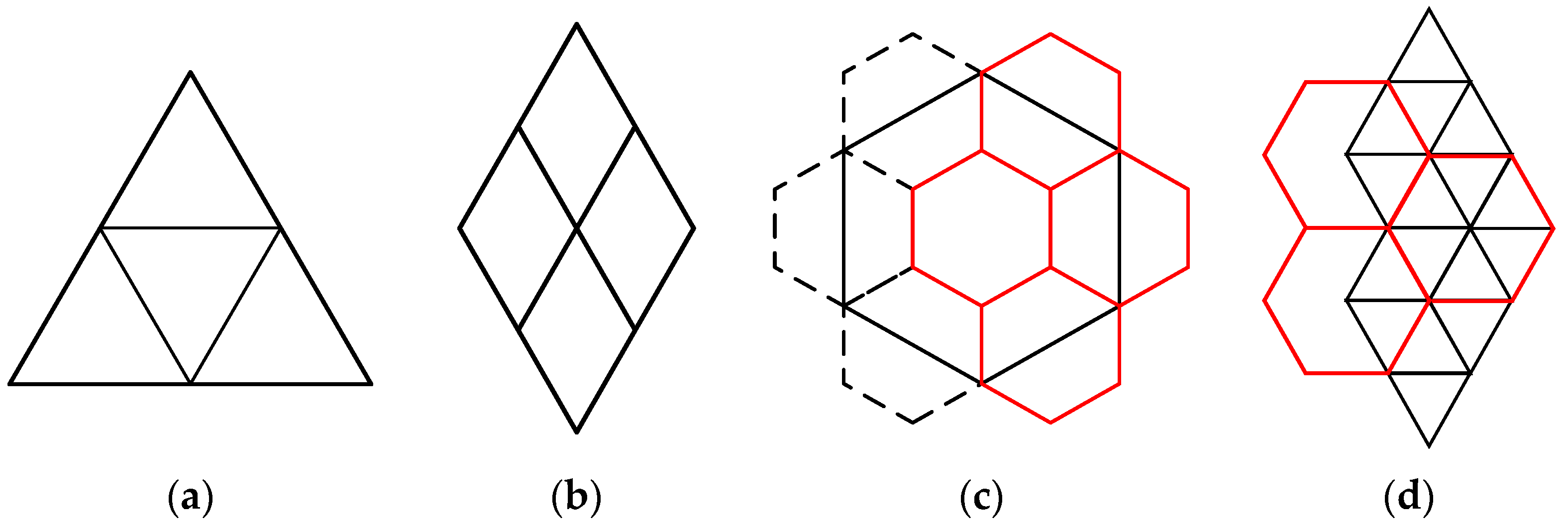
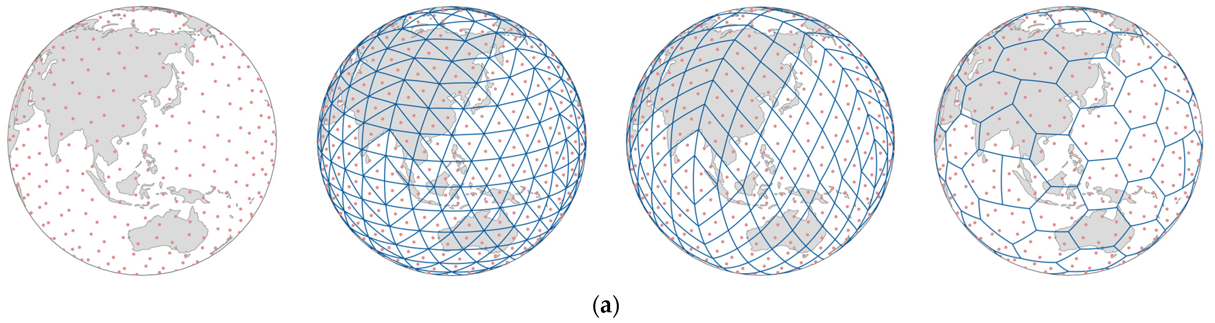
Within the Discrete Global Grid System (DGGS), scholars from around the world, after several decades of exploration and research, have designed and developed a variety of grid model systems and coding schemes. The commonly utilized shapes for global discrete grid cells include spherical triangles, diamond shapes (quadrilateral), and hexagons. Figure 2 illustrates these grids, which take on different shapes based on the octahedral structure.
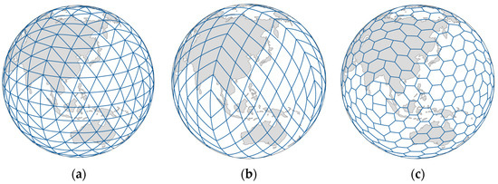
Figure 2.
Discrete Global Grid System (DGGS) with different grid shapes. (a) Triangular grid; (b) diamond grid; (c) hexagonal grid.
The subdivision of rhombus and triangular meshes is relatively straightforward, as the coverage area of the parent cells aligns perfectly with the several sub-cells of each shape, as shown in Figure 3a,b. In contrast, hexagonal grid subdivision is more complex, requiring the management of combinations involving cross-border hexagons, as illustrated in Figure 3c. Different grid types can be conveniently interconverted through corresponding relationships. Triangles and diamonds are interconvertible through merging and splitting, with a single diamond being composed of two vertically aligned triangles. Furthermore, triangles and hexagons are interconverted through a dual relationship, wherein multiple triangles are combined and staggered to form multiple hexagons, as shown in Figure 3d.
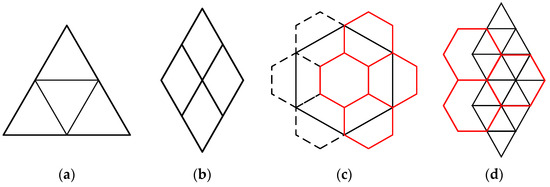
Figure 3.
Grids of different shapes [25]. (a) Triangular grid; (b) diamond grid; (c) hexagonal grid, with the red hexagon as a subunit of the black hexagon and the dashed hexagon having different parent units, ensures the uniqueness of affiliation; (d) correspondence.
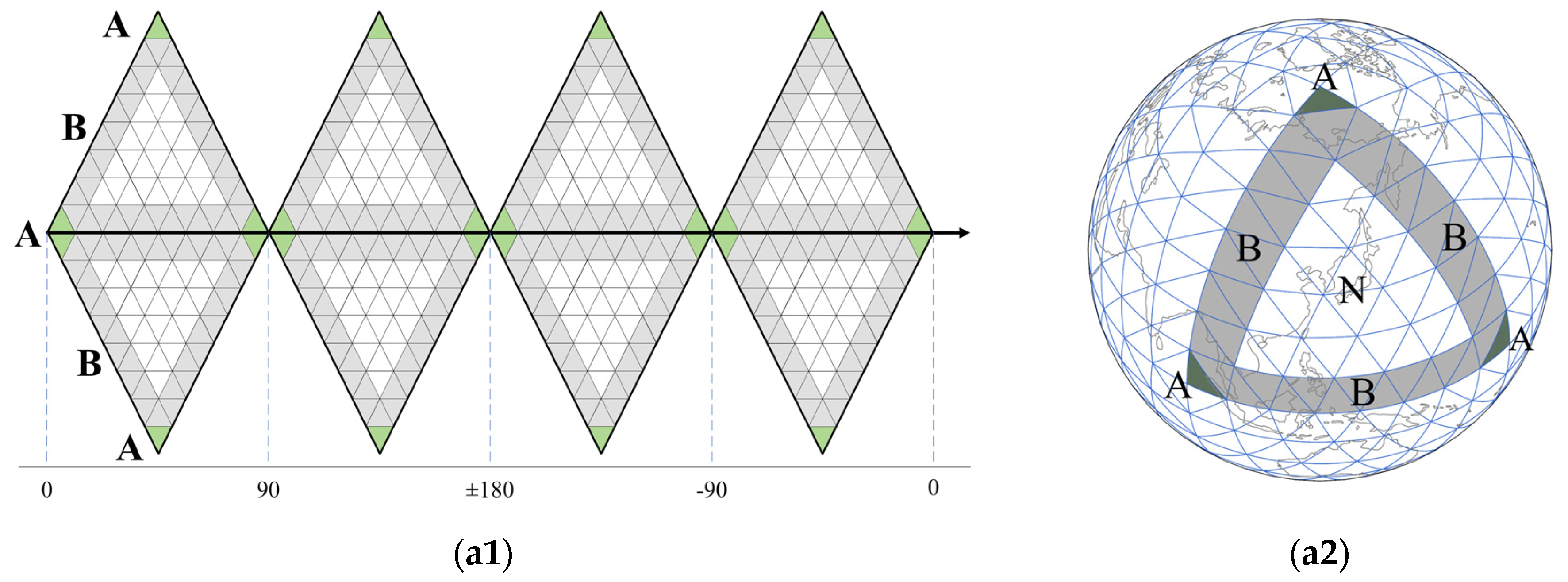
The Quaternary Triangular Mesh (QTM) system, as a type of spherical triangular grid, serves as a foundational grid within the DGGS. Initially proposed by Dutton [26], the hierarchical subdivision of the QTM is illustrated in Figure 4. The QTM exhibits favorable hierarchical and nested properties, ensuring that grid shapes and areas are approximately equal, which are characteristic features of typical grid models. The triangular grid is the most fundamental unit of a spherical grid, enabling more precise boundary fitting [27]. Compared to hexagonal grids, it offers better nesting properties. Consequently, this paper selects the QTM, based on the octahedron, as the foundational grid for the generation of spherical Voronoi diagrams.
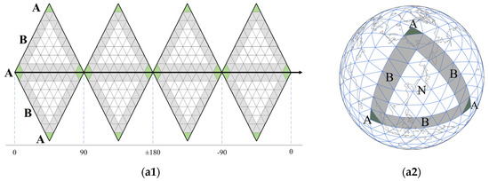
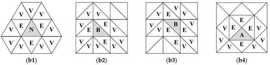
Figure 4.
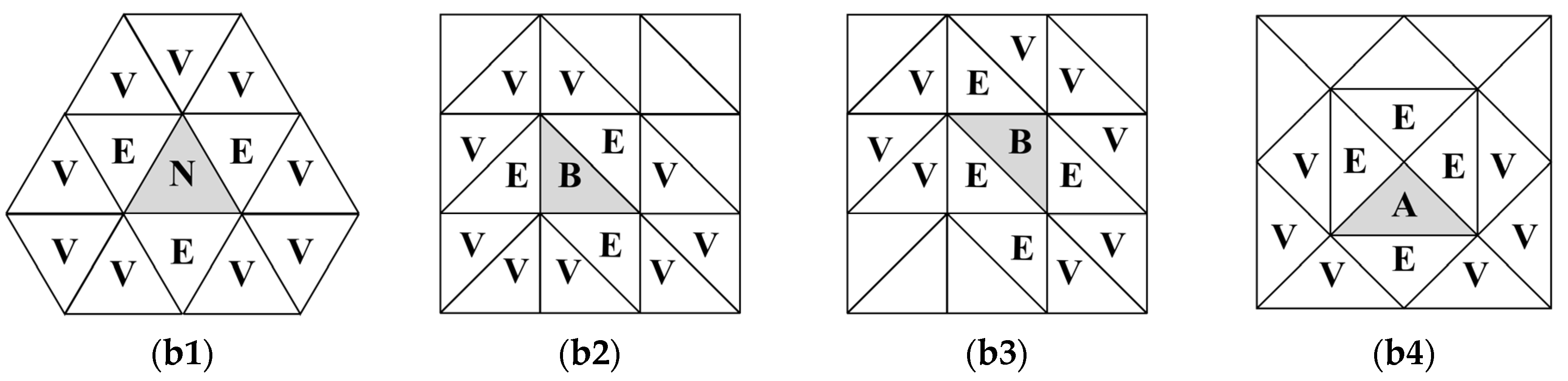
(a) Tessellation method. Gray grids located on the boundaries of the octahedral base faces (Grid B and green grids are at the vertices (Grid A). (b) neighboring triangles of QTM. The Grid E shares edge, while the Grid V shares vertex.
Within the QTM system, adjacent triangular grids that share a common edge or vertex are termed neighbor triangles (E and V). After the sphere is partitioned according to the QTM, the grids can be categorized into three types based on the topological relationships between its neighbor triangles. The first category includes the common triangular grids located within the interior of the octahedral base faces (Grid N in Figure 4a), and their topological relationships are depicted in Figure 4(b1). These grids possess four neighbor triangles in the east–west direction, three to the north, and five to the south, amounting to a total of twelve neighbor triangles. The second category encompasses triangular grids situated on the boundaries of the octahedral base faces (Grid B in Figure 4a). These exhibit two variations in topological relationships: one with four neighbor triangles in the east–west direction and two to the north and six to the south and the other with five neighbor triangles in the east–west direction and three to the north and four to the south, as shown in Figure 4(b2,b3), totaling twelve neighbor triangles. The third category comprises the triangular grids located at the apex corners of the octahedral base faces (Grid A in Figure 4a), which have ten neighbor triangles, as depicted in Figure 4(b4). For information regarding the QTM neighbor triangles search algorithm, please refer to the literature [12].
In grid space, grids are utilized as the fundamental units to represent points, and a series of neighboring grid units are employed to approximate the representation of regions. The measurement of distance within grid space, the great-circle distance or ellipsoidal distance between grid center points, does not entirely correspond to the point-to-point distances found in vector space, inevitably introducing a certain degree of error into the process [14]. It is commonly accepted that the most ideal outcome in representing spherical elements is to limit the error within the confines of a single spherical grid. The grid of QTM, with its attributes of multi-resolution and infinite subdivision, allows for precision control by adjusting the grid resolution to balance efficiency requirements and specific application demands in practical applications.
2.2. Principle of the Algorithm
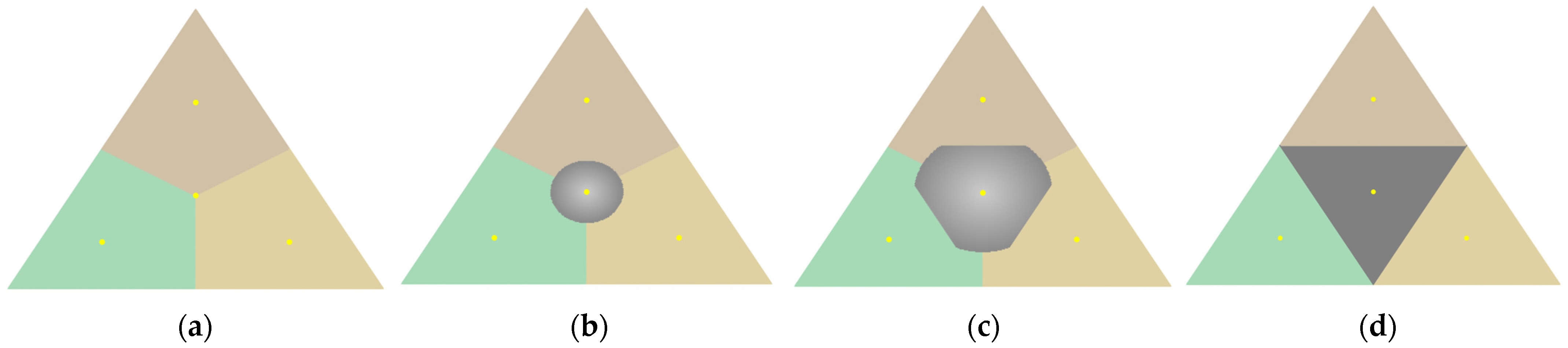
The fundamental principle underlying the algorithm presented in this paper is the design of a dilation canonical ordering strategy for the spherical triangular grid. The strategy facilitates an ordered outward expansion centered on point, line, and surface grid cells, enabling the construction and updating of the spherical Voronoi diagram, as depicted in Figure 5. The procedure initiates with the insertion of a new generation point, as shown in Figure 5a; it then undergoes outward dilation, propagating distance changes to neighboring cells, as illustrated in Figure 5b. The dilation process terminates, and propagation stops when it encounters grid cells that are equidistant from other generation points, ensuring that the distance change no longer affects the subsequent cell in the direction of dilation, as portrayed in Figure 5c,d. Ultimately, the dilation of the grid effectively delineates the updated region. The dilation not only enables the updating of local areas but also facilitates the construction of the entire spherical Voronoi diagram.

Figure 5.
Voronoi diagram update based on grid dilation. (a) Initial, representing different Voronoi regions with different colors; (b) beginning, Wherein the dilated area is indicated by the color gray; (c) process; (d) result.
Tailored to the characteristics of the algorithm and the multi-level attributes of the spherical triangular grid, this paper designs the data structure and expansion sorting strategy as follows:
2.2.1. Data Structure
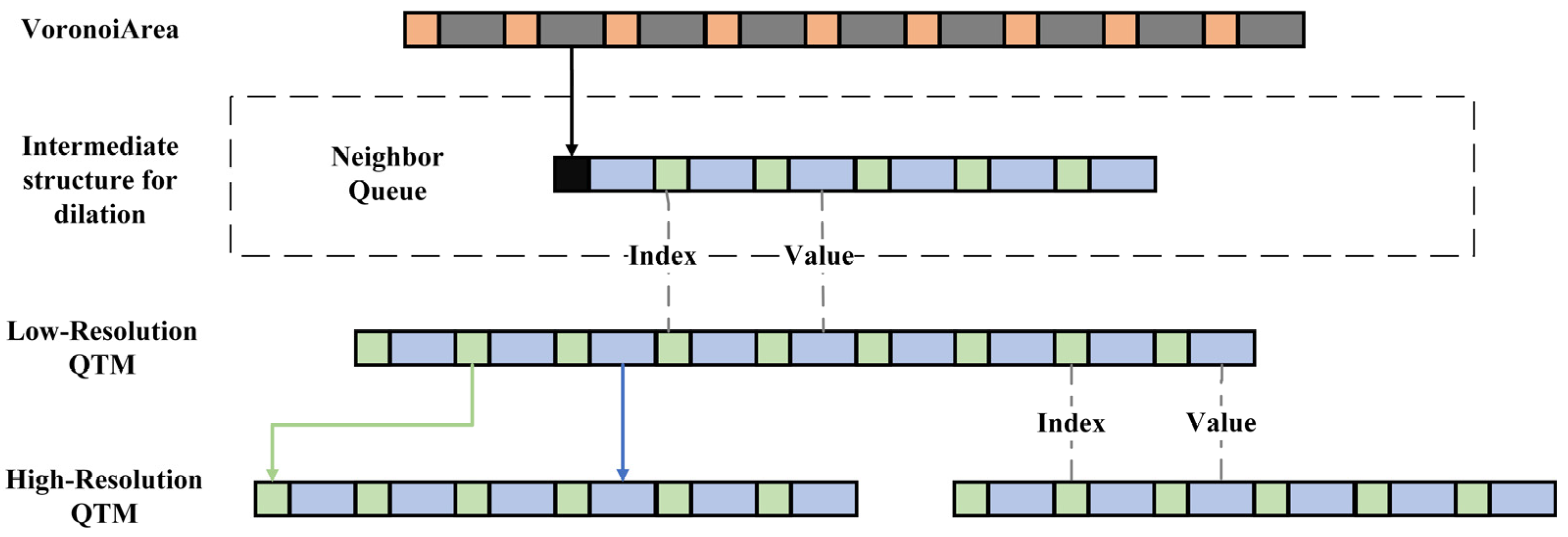
The overall data structure of the algorithm is a three-tiered architecture composed of dictionaries and queues, as depicted in Figure 6. The first tier pertains to the structure of the Voronoi regions, functioning to store growth point sites and to index the dilation queues. Each site is associated with a corresponding dilation queue. The second tier comprises the dilation queues (designated as dilationQueue), which act as an intermediate data structure in the generation of the Voronoi diagram, housing information on the dilated neighborhood grids. Here, the keys correspond to grid codes, while the values contain the site codes and their associated expansion grid properties. The third tier involves the QTM grid structure (called QTMDict), which is responsible for storing Voronoi attributes, with keys again corresponding to grid codes and values storing the respective Voronoi site codes and grid properties. The construction of the Voronoi diagram is considered complete once all QTM grids have been accurately assigned Voronoi region codes. Additionally, the third tier incorporates a multi-resolution QTM data structure designed to accommodate potential visualization and application requirements.

Figure 6.
Data structure. Orange represents sites, gray represents the dilation queue, green represents keys storing grid numbers, and blue represents values storing site codes and grid properties.
Each site is associated with a DilationQueue, which serves to store temporary information of the neighborhood grids involved in the dilation process. The grids within this queue originate from the neighborhood grids resulting from prior dilation operations and are also designated as the target grids for subsequent dilation operations. During each dilation operation, a grid is retrieved from the queue, subjected to a dilation operation, and subsequently, the neighboring grids influenced by this operation are placed back into the queue in preparation for the subsequent round of propagation.
2.2.2. Spherical Grid Ordering Strategy
Canonical ordering is a method employed for the rearrangement of matrices. It restructures the rows and columns of a matrix to enhance its structural properties, thereby facilitating more efficient analysis and indexing. Owing to the exceptional performance of canonical ordering in reducing the search space, this strategy is utilized in this paper to direct the directionality and sequencing of the dilation process of grids of QTM during the construction of Voronoi diagrams.
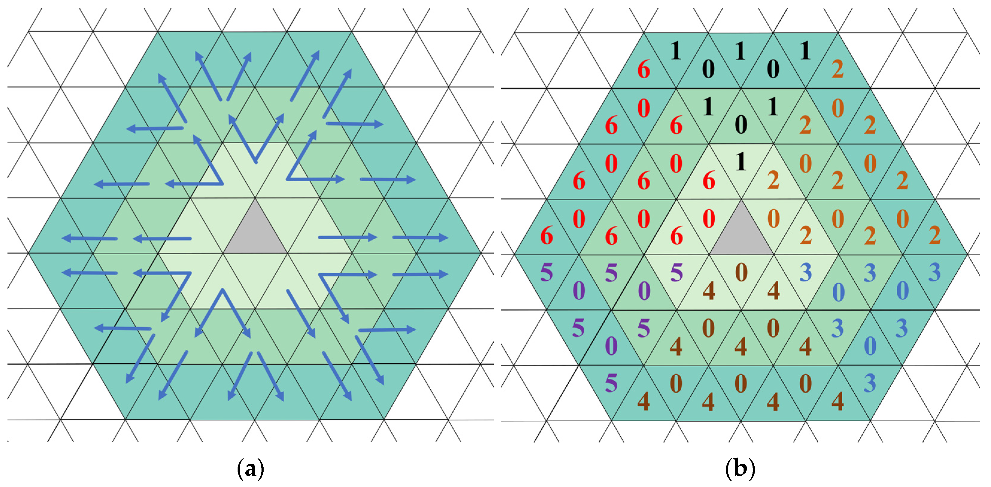
The topologies of spherical and planar structures differ, making the expansion strategy of a planar square grid unsuitable for the sphere. For the QTM, as a spherical triangular grid, we have designed six basic dilation directions, as shown in Figure 7. With this canonical ordering rule, the gray grid cell is centered and dilation occurs outward along the blue arrows, ensuring that most grid cells are visited only once. Similarly, to label different grid dilation directions, we have defined seven grid attributes, termed GridType, labeled consecutively from 0 to 6, with each GridType corresponding to a distinct base dilation direction, as depicted in Figure 7b. For instance, a grid with GridType set to 1 (referred to as Grid1) expands towards three grids in the north direction. When the dilation process reaches Grid1, it is removed from the dilationQueue, and the three northern grids are then placed into the dilationQueue, each assigned GridType 0 or 1. Upon operating on a new Grid1, the northern grids of this new Grid1 are also placed into the queue, facilitating the northward expansion of Grid1. Grid2-6 are assigned dilation directions in a similar fashion, each expanding in a systematically ordered outward direction based on their respective GridType. In contrast, Grid0, when extracted from the queue, undergoes computational and judgmental operations without actual dilation. Figure 7 illustrates a dilation process centered on an upright triangle, with the dilation direction of the inverted triangle being mirror-symmetric to that of the upright triangle, and thus, is not elaborated further. The QTM neighborhood search method, neighborsSearchAlgorithm(), is detailed in the literature [12]. In this paper, the aforementioned canonical sorting strategy is encapsulated within the function findSuccessors(). The pseudocode for the canonical sorting algorithm findSuccessors() is presented in this paper, as shown in Algorithm 1.
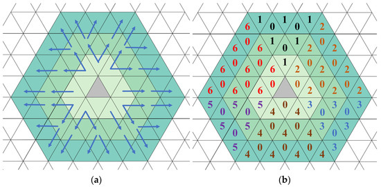
Figure 7.
Dilation ordering rule based on QTM. Numbers in different colors, which correspond to the respective arrows, represent different dilation directions. Different shades of green represent different levels of neighborhoods.
In the Discrete Global Grid System, polylines and polygons are considered as being composed of a series of grids. The ordered dilation of polylines and polygons is achieved through the ordered dilation of each individual grid cell. As shown in Figure 8, the generator is a polyline composed of a series of grid cells, represented by the gray grids. The dilation begins from grid a, expanding northward to Grid1, northeastward to Grid2, southeastward to Grid3, southwestward to Grid5, and northwestward to Grid6. Next, grid b is processed, except for the grids that have already been dilated, expanding to Grid2 in the northeast, Grid4 in the south, Grid5 in the southwest, and Grid6 in the northwest. The process then moves to grid c, and so on. After all the gray grids have been dilated, the first neighborhood grid cells, represented in light green, are assigned their respective dilation directions. The next round of dilation targets the second neighborhood grid cells in green, assigning dilation directions to each grid cell, followed by the third neighborhood grid cells in teal.
| Algorithm 1: Pseudocode for the findSuccessors() function |
| Input: gIn: input grid, gtIn: the grid type of gIn |
| Output: gOut: the successor grids, gtOut: the grid type of gOut |
| 1. switch gtIn do |
| 2. case a value of gridType do |
| 3. gOut ← neighborsSearchAlgorithm(gIn) |
| 4. w = whether crossed the vertexes of fundamental plane in neighborsSearchAlgorithm() |
| 5. gtOut ← gridType(w, gtIn) |
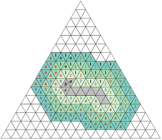
Figure 8.
The dilation of a polyline. Numbers in different colors represent different dilation directions. Different shades of green represent different levels of neighborhoods.
The dilation algorithm introduced in this paper does not expand uniformly in all directions during the dilation process. Instead, it employs the findSuccessors() function to filter neighboring grid cells based on canonical ordering principles. As depicted in Figure 7, only grids aligned with the indicated arrow directions are chosen as candidates for the subsequent round of dilation, while other grids are disregarded. Under most circumstances, each affected cell is visited solely once, thereby eliminating the computational redundancy associated with indiscriminate expansion and significantly enhancing the algorithm’s efficiency.
2.2.3. Treatment at the Boundary of the QTM Foundation Surface
The QTM is constructed from eight fundamental faces of an octahedron, which collectively form the surface of a sphere. As the grid dilation process crosses the boundaries of these base faces, the topological relationships undergo changes. Consequently, the directions for the ordered dilation of the grid must be correspondingly adjusted, necessitating special handling.
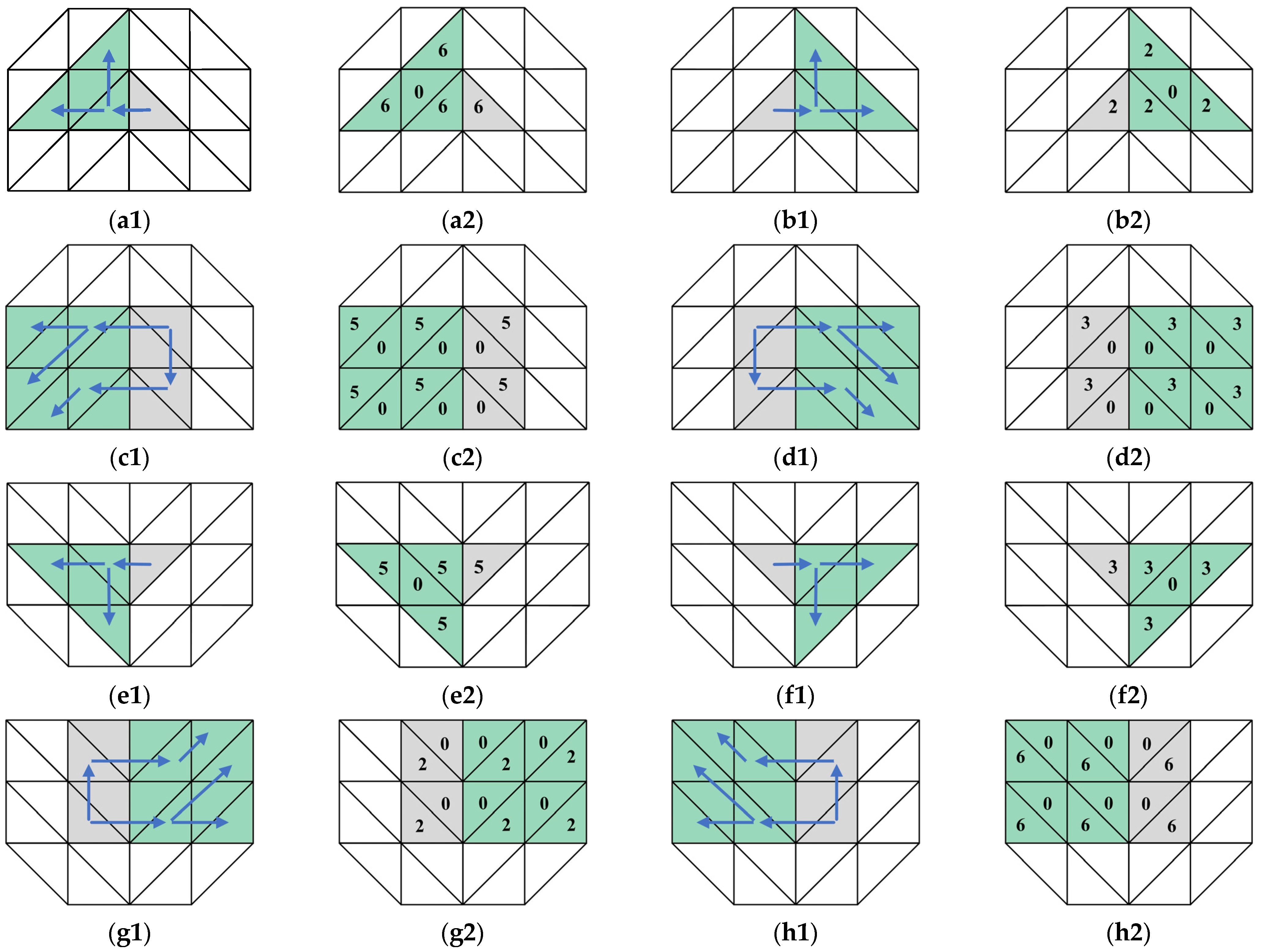
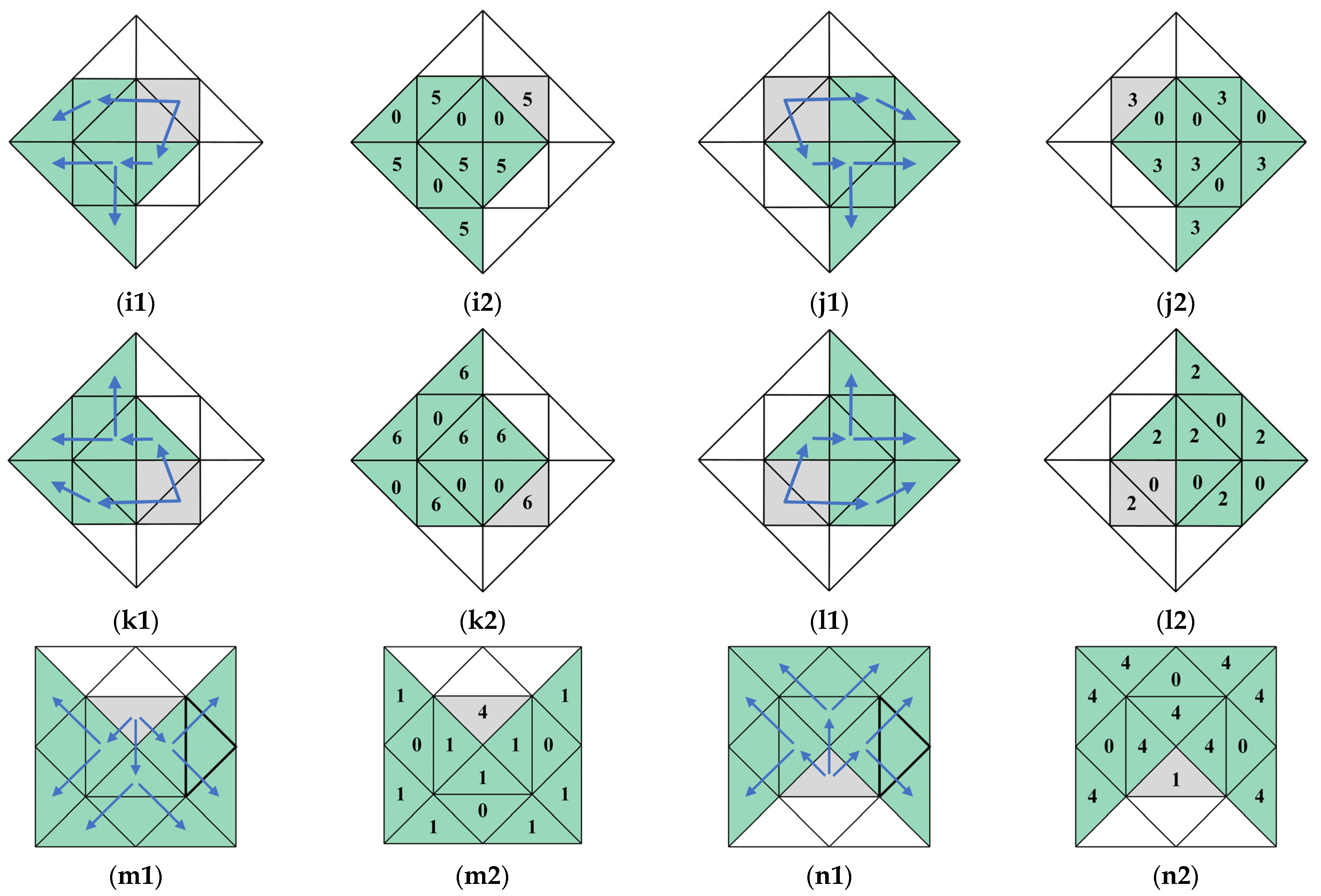
In the northern hemisphere, the grid of QTM undergoes dilation towards the northwest direction, crossing the boundary of a base plane (grid B in Figure 4). The gray Grid6 in Figure 9a, and its western neighboring grid, which is also an upright triangle, are initially dilated and assigned GridType 6. The dilation then proceeds in the northwest direction, as depicted by the green grids in Figure 9(a2). Similarly, when the dilation direction is towards the northeast and crosses the base plane boundary, the resulting dilation is shown in Figure 9b. When the dilation direction in the northern hemisphere is towards the southwest and crosses the base plane boundary, the gray Grid5 in Figure 9c transfers GridType 5 to the grid directly to its south and assigns GridType 0 to the first two grids to its west. The third grid to the west is given GridType 5. The grid then continues to propagate in the southwest direction. The dilation towards the southeast direction across the base plane boundary yields results, as shown in Figure 9d. In the southern hemisphere, the dilation directions and operations are mirror images of those in the northern hemisphere, as illustrated in Figure 9e–h.
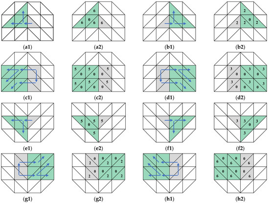
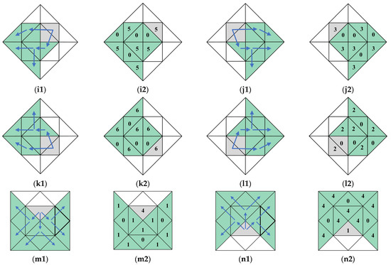
Figure 9.
Treatment at the boundary of the QTM foundation surface. Gray represents the initial grid, green represents the target grid for dilation, and the arrows corresponding to different numbers indicate the directions of dilation.
Figure 9i illustrates the dilation operation when the southwestward expansion crosses the angle formed by the base plane boundary and the equator (grid A in Figure 4). The gray Grid5 undergoes dilation affecting a southern grid with GridType 5, as well as three western grids—two are labeled GridType 0 and one is labeled GridType 5. Figure 9j–l depict the dilation operations when expansion traverses the angles at the boundaries with the equator in the northwest, southeast, and southwest directions, respectively. When the dilation process reaches the spherical poles, the direction of dilation inverts. As depicted in Figure 9n, upon reaching the North Pole, the dilation starts expanding towards the south, and the GridType is modified from 1 to 4; conversely, upon reaching the South Pole, the dilation shifts to expand towards the north, and the GridType is switched from 4 to 1.
2.3. Algorithm Process
2.3.1. Initialization
Algorithm 2 presents the pseudocode for the initialization phase in the construction of a Voronoi diagram. The function buildQTMGrids() is utilized to establish the foundational framework of the QTM. This encompasses processes such as grid partitioning, grid encoding, and the computation of coordinates of grid points. Subsequently, each generated point, denoted as sites[i], is sequentially inserted into the dilationQueue. For every sites[i], a dilationQueue[i] is instantiated. Concurrently, the generated points are stored within the QTMDict, with the gridType initialized to 0, designating each point as the nearest growth site.
| Algorithm 2: Pseudocode for the initialization section |
| Input: sites: the sites of Voronoi diagram |
| 1. buildQTMGrids() |
| 2. for each sites[i] in sites do |
| 3. put sites[i] in dilationQueue[i] |
| 4. gridType← 0 |
| 5. site ← i |
| 6. QTMDict [sites[i]] ← gridType, site |
2.3.2. Ordered Dilation
The pseudocode outlining the steps of the algorithm’s ordered expansion process is presented in Algorithm A1 of Appendix A. The specific procedural steps of the algorithm are as follows:
- Initial Dilation. The initial dilation step involves adding the neighboring grids of the growth point site, referred to as siteNeighbor, into the dilationQueue. Each grid within siteNeighbor is assigned a gridType to prepare for the subsequent ordered dilation process. The siteNeighbor consists of grids labeled Grid1-6 and three instances of Grid0, making a total of twelve grids. This collection of grids, siteNeighbor, marks the starting point for all subsequent ordered dilations. Following the initial dilation, the resulting configuration of siteNeighbor and its gridType are stored in the QTMDict. The origin of the dilation, identified as site, is recorded as the closest growth point. Once the initial dilation is complete, the growth point is extracted from the dilationQueue. (This process is detailed in lines 1 to 7 of Algorithm A1 in Appendix A.)
- Ordered Dilation. Sequentially, grids are taken from the dilationQueue[i] and are marked as g. Using the findSuccessors() function, the new dilation cell gridSuccessor for the current grid g is identified based on its gridType. The gridType of gridSuccessor is then stored in the QTMDict. The site of its dilation originator is set to the nearest growth point. (This process is outlined in lines 8 to 14 of Algorithm A1 in Appendix A).
- Repeated Dilation Process. The dilation process is repeated until the dilated regions from different growth points intersect. The spherical distances from the intersecting grid to each of the two growth points are computed individually, denoted as disNew and disOld. If disNew is less than disOld, the grid will be incorporated into the dilationQueue associated with the growth point corresponding to disNew. The dilation continues until disNew exceeds disOld, indicating that the dilation has reached the midpoint between the two growth points, when the dilation is terminated. Here, Dist() represents the function for calculating the spherical distance.
- Termination of Dilation Process. The dilation process is halted when the dilationQueue[i] becomes empty. At this juncture, within the QTMDict, each grid cell has stored the nearest growth point site. This indicates that the grids belong to the Voronoi region represented by the site. All grids that share the same growth point are aggregated into the same Voronoi region, and the union of these distinct Voronoi regions constitutes the entire Voronoi diagram.
In grid space, lines and surfaces are represented by a series of grids, and the dilation of lines and surfaces is carried out in the same manner as the dilation of points set. In the process of ordered dilation, no distance calculations are performed until the different dilations meet and the spherical distances between them are calculated and compared. The dilation of the shorter distance continues until the distances between the two are approximately equal. This method ensures that the error in the generated Voronoi diagram is contained within one grid.
It is important to note that when constructing a Voronoi diagram for a localized region on the sphere rather than the entire spherical surface, irregular boundaries of the region may impede the propagation of ordered dilation. Consequently, in the construction of a Voronoi diagram for a localized spherical area, once the dilation reaches the boundary of the region, the ordered dilation is aborted. Instead, dilation is modified to proceed in all directions along neighboring grids to prevent the omission of grids.
2.3.3. Voronoi Diagram Update Procedure
Algorithm A2 presents partial pseudocode for the update of Voronoi diagrams. It is composed of two fundamental operations, insert() and delete(), both of which are facilitated by the ordered dilation process, orderedDilate().
In the insertion operation, the process commences with an initialization step. The grid to be inserted is added to dilationQueue and QTMDict. The nearest site is set to the grid itself. It is crucial to ensure that the identifier assigned to the inserted sites is differentiated from the identifiers of the existing sites to avoid any confusion or errors. (This corresponds to lines 1 through 4 of Algorithm A2.) Subsequently, the orderedDilate() function is utilized to perform an orderly dilation, until a grid cell equidistant from other sites is encountered, thereby halting further propagation.
When a delete operation is performed, two dilation operations are performed. Initially, the process begins with initialization, where the grid designated for deletion, referred to as deleteSites, is added to the dilationQueue[ds] (corresponding to lines 6 to 9 of Algorithm A2). Subsequently, an ordered dilation is performed to locate all grids nearest to deleteSites. The nearest sites are then set to null, which signifies that the attributes of all grids and sites corresponding to deleteSites are rendered invalid (corresponding to lines 10 to 18 of Algorithm A2). Ultimately, the dilation process is reinitiated from the opposite side of the boundary. This continues until the previously invalidated area is fully covered once more.
3. Experiment
The programming language utilized for the algorithm presented in this paper is Python (3.9.0). The three-dimensional visualization is accomplished using the Matplotlib toolkit. Calculations for spherical and ellipsoidal distances are facilitated by the PYPROJ library. The hardware environment consists of an 11th Gen Intel(R) Core(TM) i5-1135G7 @ 2.40 GHz, with 24.0 GB of RAM.
3.1. Feasibility and Completeness of the Algorithm
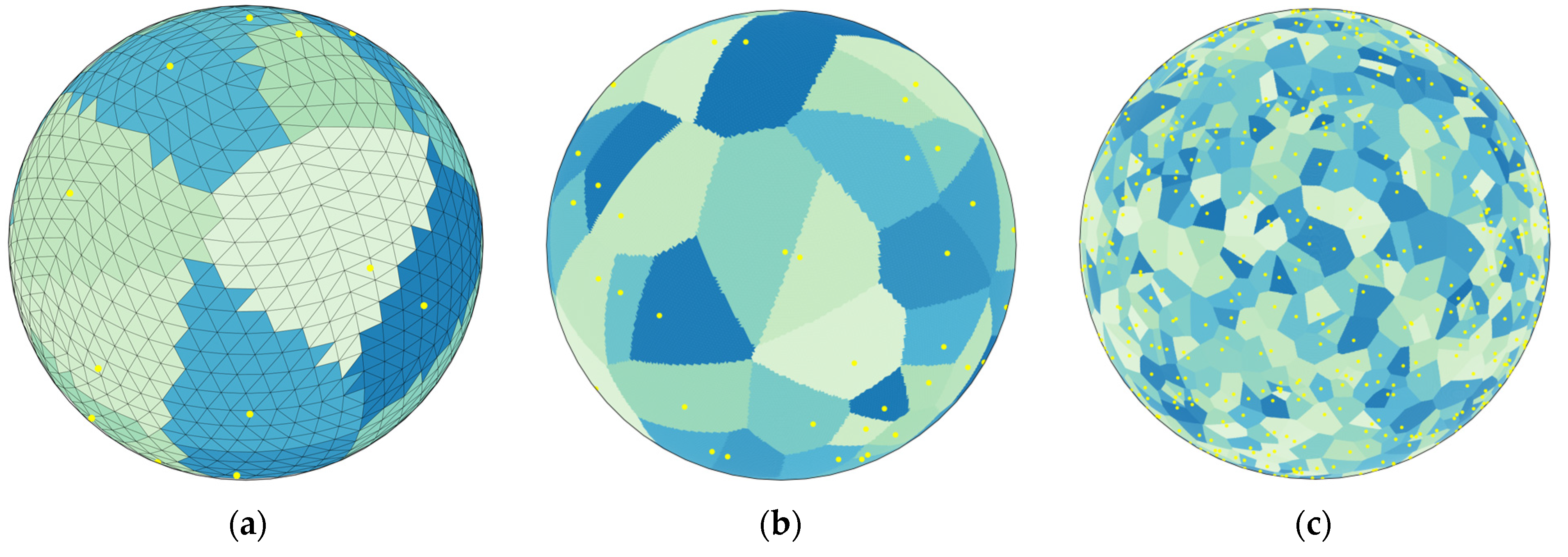
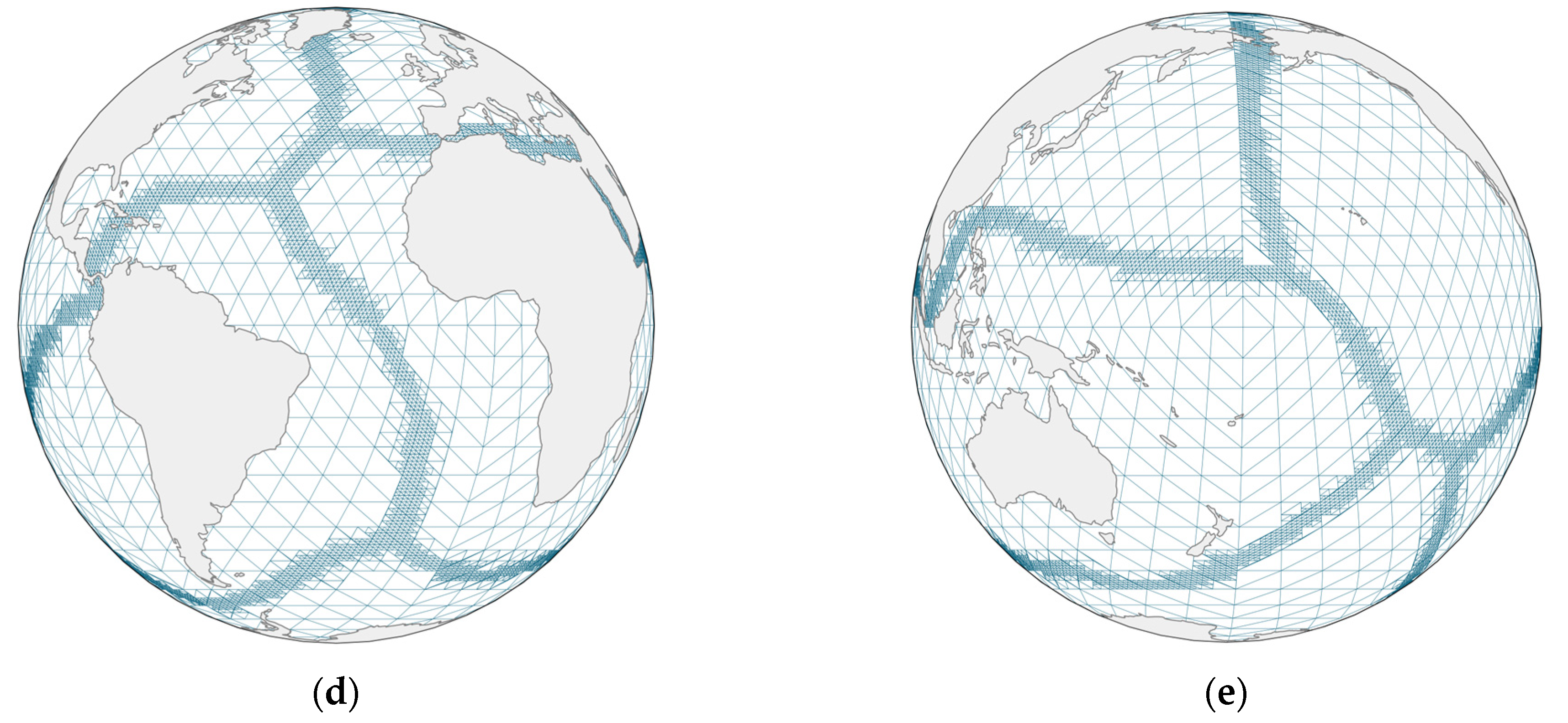
This paper conducts an experimental validation of the feasibility of the proposed method. Figure 10a–c present illustrations of the results generated by the ordered expansion algorithm under various grid levels and different numbers of generation points. Figure 10d,e showcase illustrations of the spherical Voronoi diagrams constructed by the algorithm, utilizing the major landmasses as the generation surface.


Figure 10.
Spherical Voronoi diagrams’ generation results. (a–c) Generated by spherical points, where different colors represent different Voronoi regions. (d,e) Generated by major landmasses.
An experiment is designed to measure the error by directly applying the definition of Voronoi, which involves randomly sampling points on the boundary lines and calculating the absolute value of the distance difference between the sampled points and the two sides of the Voronoi generator. As shown in Figure 11, the boundary points, represented by red dots, are randomly located on the shared edges of adjacent grid cells. The yellow dots represent the Voronoi generators. The spherical distances between these points and their respective Voronoi generators, indicated by black lines, are used to calculate the Voronoi error, which is the absolute difference between these two distances.
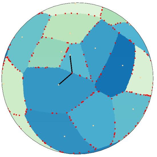
Figure 11.
Voronoi error calculation. The red points represent boundary points, the yellow points represent generators, with different colors indicating different Voronoi regions.
Equation (1) is used to calculate the algorithm error results. In the equation, the function is utilized to compute the spherical distance between the generator and the boundary point, and represent the two sides of the Voronoi generator, means the randomly sample point on the boundary line, and denotes the maximum edge length of the grid at the current hierarchical level.
Due to the close relationship between error magnitude and grid cell size, is defined as the ratio of the error to the edge length of the grid cell. Since the grid cells at the same level have slight variations in size and edge length, we select the maximum edge length of the grid cells as the evaluation standard. It should be noted that the maximum grid edge length at each level is approximately 1.5 times the average edge length. The experimental results of the algorithm’s error are depicted in Table 1, with the 6th, 7th, 8th, 10th, and 14th levels of QTM serving as the foundations.

Table 1.
Error analysis through the distance calculation.
As shown in the results, the error for most boundary random points falls within the range of 0 to 0.3. The error of all boundary points is confined within one grid cell of the corresponding hierarchical level, i.e., the error is less than 280,006 m at level 6 and less than 18,086 m at level 10. By increasing the subdivision level locally, according to the specific needs, the error can be controlled more precisely.
The algorithm by Kazemi et al. [15] has demonstrated its accuracy through experimental validation. The spherical distance transformation produced by their method exhibits only minor errors when compared to the results generated by ArcGIS Pro, which can be disregarded. This study reproduces their algorithm and employs the same spherical distance calculation tool used in our algorithm. The spherical results of their algorithm are utilized as a benchmark for the accuracy assessment of our algorithm’s results.
This paper employs Equation (2) to calculate the error of the algorithm’s results. In the equation, the function Dist(a, b) is utilized to compute the spherical distance between the site and the grid, and and represent the closest growth points calculated using the algorithm presented in this paper and Kazemi’s algorithm, respectively. L denotes the average edge length of the grid at the current hierarchical level. The experimental results of the algorithm’s error are depicted in Table 2. The experiments are based on a set of 100 sites that are randomly distributed across the surface of a sphere, with the 7th, 8th, 9th, and 10th levels of QTM serving as the foundations.
Table 2.
Errors analysis of algorithm.
As can be observed, using Kazemi’s algorithm as a benchmark, the Voronoi diagrams generated by the algorithm presented in this paper have controlled the error within one grid. Given that raster data inherently possess an error equivalent to one grid cell in expressing geospatial entities, the algorithm proposed is considered to have achieved a comparable level of accuracy to Kazemi’s algorithm. This affirms the completeness of our algorithm.
3.2. Efficiency Evaluation
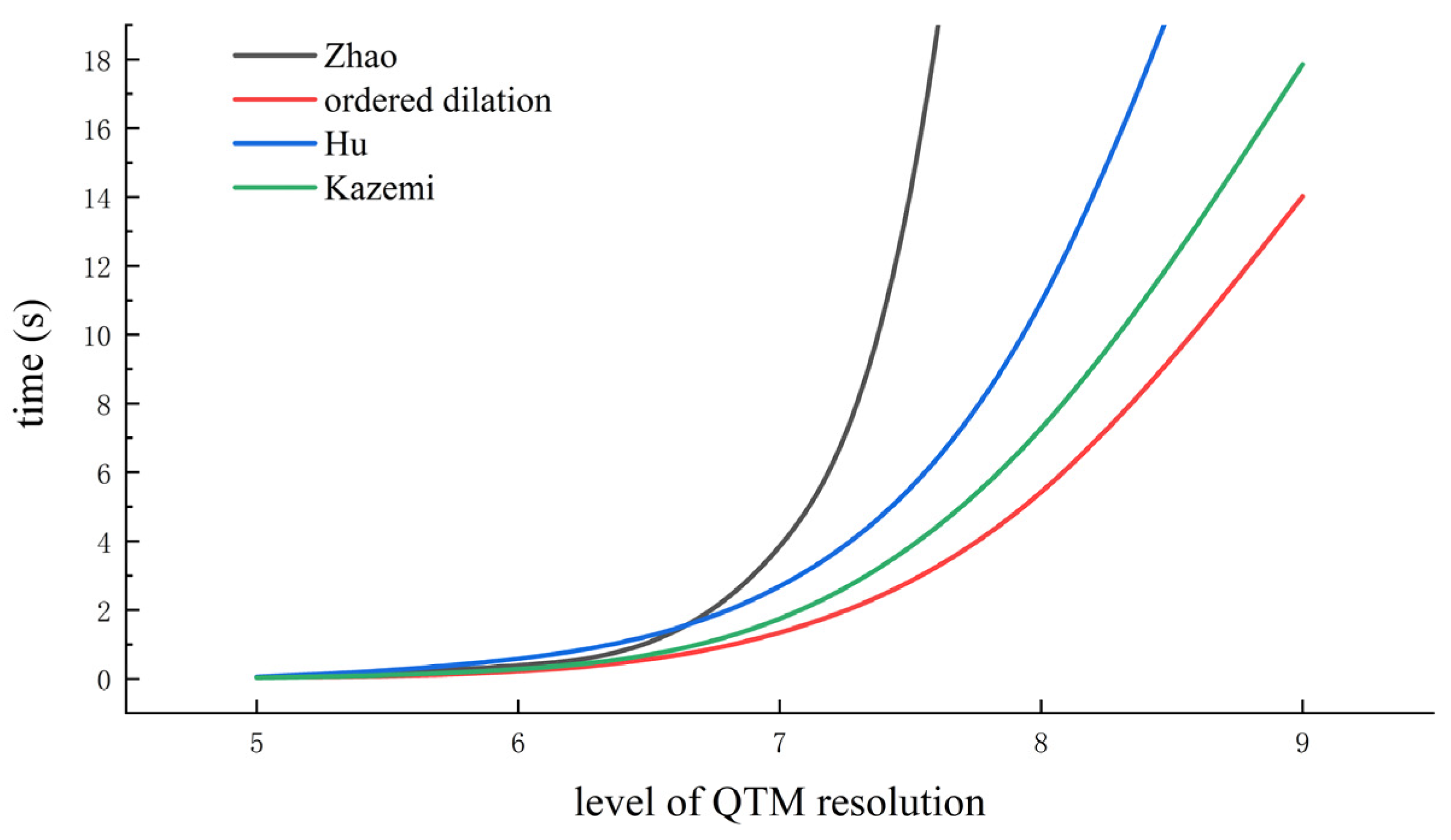
This paper reproduces the algorithms of Kazemi [15], Zhao [12], and Hu [14] and conducts efficiency comparison experiments with them. The reproduced algorithms of others adopted the same distance metric as this paper and utilized the same spherical toolbox. The sites consist of a set of 100 randomly distributed spherical points. The experimental results of the overall construction of the spherical Voronoi diagram are presented in Table 3 and illustrated in Figure 12. Figure 12 represents the time required by the algorithm, while the horizontal axis delineates the levels of the QTM. It should be noted that Hu’s algorithm is predicated on a planar grid; hence, the time recorded for Hu’s algorithm is under an equivalent number of grids. The experimental results demonstrate that, in the context of constructing a complete spherical Voronoi diagram, the efficiency of the ordered dilation algorithm proposed in this paper is significantly higher than that of Zhao’s algorithm and slightly superior to the algorithms of Kazemi and Hu. Overall, the efficiency of our algorithm is broadly considered to be on par with the algorithms of Kazemi and Hu in terms of overall efficiency.
Table 3.
Generating times of different algorithms.
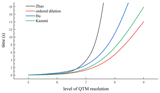
Figure 12.
Efficiency comparison of different algorithms for generating spherical Voronoi diagrams.
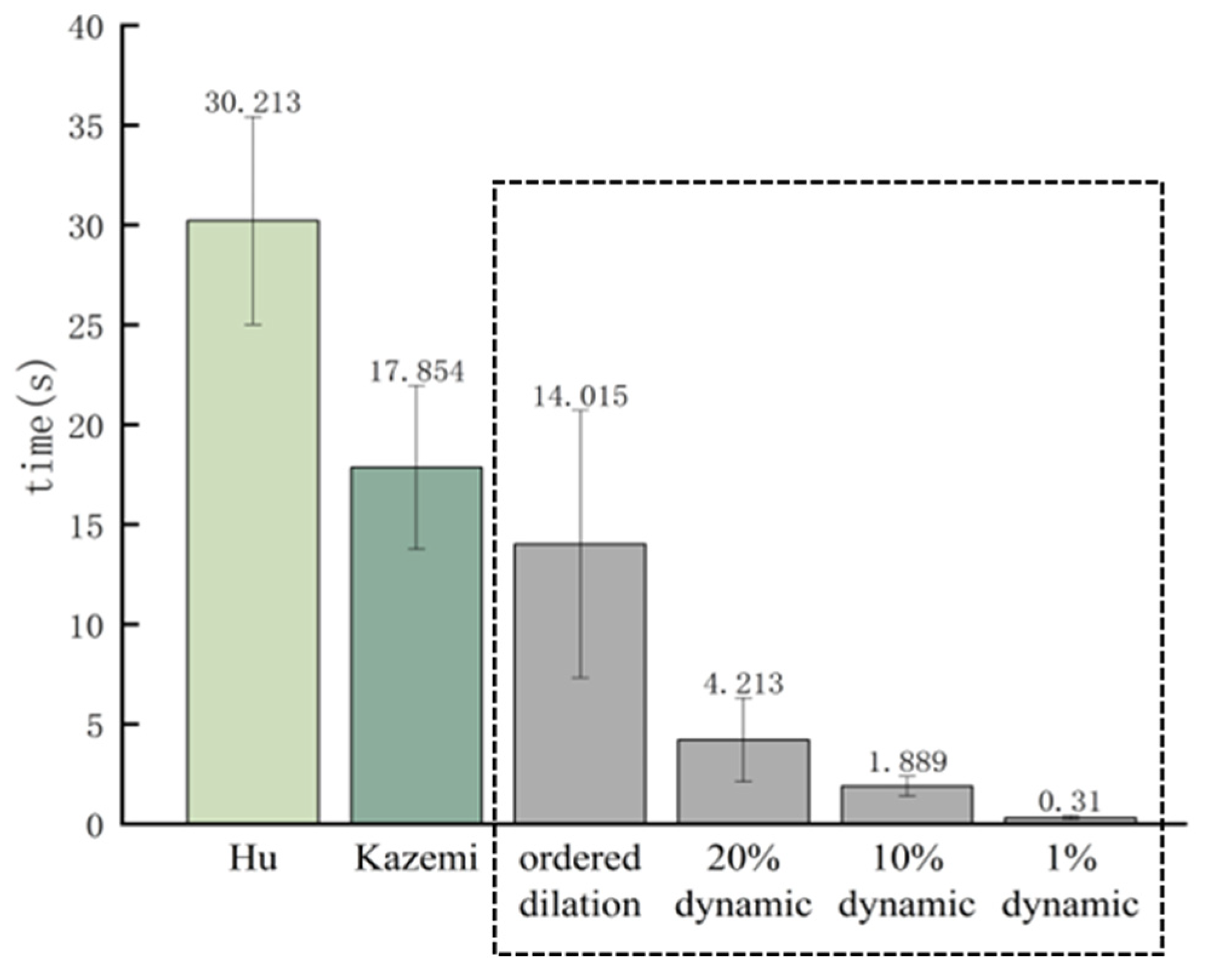
Similarly, for scenarios where changes occur in local environments, the algorithm presented in this paper is capable of selectively updating the affected regions without the need for a complete reconstruction of the Voronoi diagram. An efficiency comparison experiment was conducted, based on a nine-level QTM, consisting of 2,097,152 grids, with 100 random spherical points serving as the sites. This paper has designed four distinct scenarios: In the first scenario, all sites undergo changes, necessitating the construction of an entirely new spherical Voronoi diagram; in the second scenario, the coordinates of 20% of the sites are altered, which includes operations such as insertions, movements, or deletions; in the third scenario, the coordinates of 10% of the sites are changed; and in the fourth scenario, the change affects 1% of the sites. Figure 13 presents the time required by the algorithms of Hu and Kazemi and the algorithm proposed in this paper for the first scenario, as well as the time consumed by our algorithm for the second, third, and fourth scenarios. In the second, third, and fourth scenarios, the algorithms of Hu and Kazemi are not readily amenable to localized updates, resulting in an invariant expenditure of time. The experimental results substantiate that our proposed update algorithm can effectively enhance efficiency when changes occur in localized environments.

Figure 13.
Comparison of algorithm efficiency in different scenarios. The content within the dashed boxes represents the results of the algorithms in this paper.
From the perspective of time complexity, when reconstructing the entire spherical Voronoi diagram, the algorithm presented in this paper, as well as the algorithms by Hu and Kazemi, exhibit a time complexity of O(n), where n is the number of spherical grids. In the context of dynamic updates, our algorithm’s time complexity is O(m), where m is the number of grids requiring updates. Should the area experiencing dynamic changes be considerably smaller than the entire domain, that is, when m is much less than n ((m << n), the efficiency can be significantly enhanced. The current best vector algorithms have time complexity O(n), where n depends on the number and shape of spatial objects. Given the distinct logical constructs inherent in vector and raster algorithms, a straightforward comparison based on time complexity alone is not feasible.
3.3. Application Examples of Dynamic Navigation and Management for Ocean Vessels
Voronoi diagrams are extensively utilized in the fields of maritime navigation and vessel management [28,29,30]. By employing Voronoi diagrams, a series of distance-based boundary lines can be generated in maritime areas. This approach facilitates the analysis of ship distribution and aids in the planning and optimization of shipping routes. It ensures safe distances between vessels and coordinates their direction of travel to prevent congestion and navigate around obstacles, such as land, reefs, and other ships. Furthermore, the analysis of Voronoi diagrams enables rapid emergency response and rescue operations and allows for the more effective management of maritime resources, including the identification of the nearest rescue points, oil platforms, and fishing resources.
Taking into account the advancing automation in maritime navigation and the imperatives for safety and real-time capabilities within practical applications, this application calls for an algorithm that is not only highly precise but also efficient. To achieve this, it is essential to integrate a variety of data types and sources, including weather and vessel information, within a cohesive framework. Furthermore, the application necessitates the multi-scale construction of Voronoi diagrams and the real-time, dynamic updating of Voronoi diagrams.
3.3.1. Dynamic Construction of Spherical Voronoi Diagrams and Ship Routing
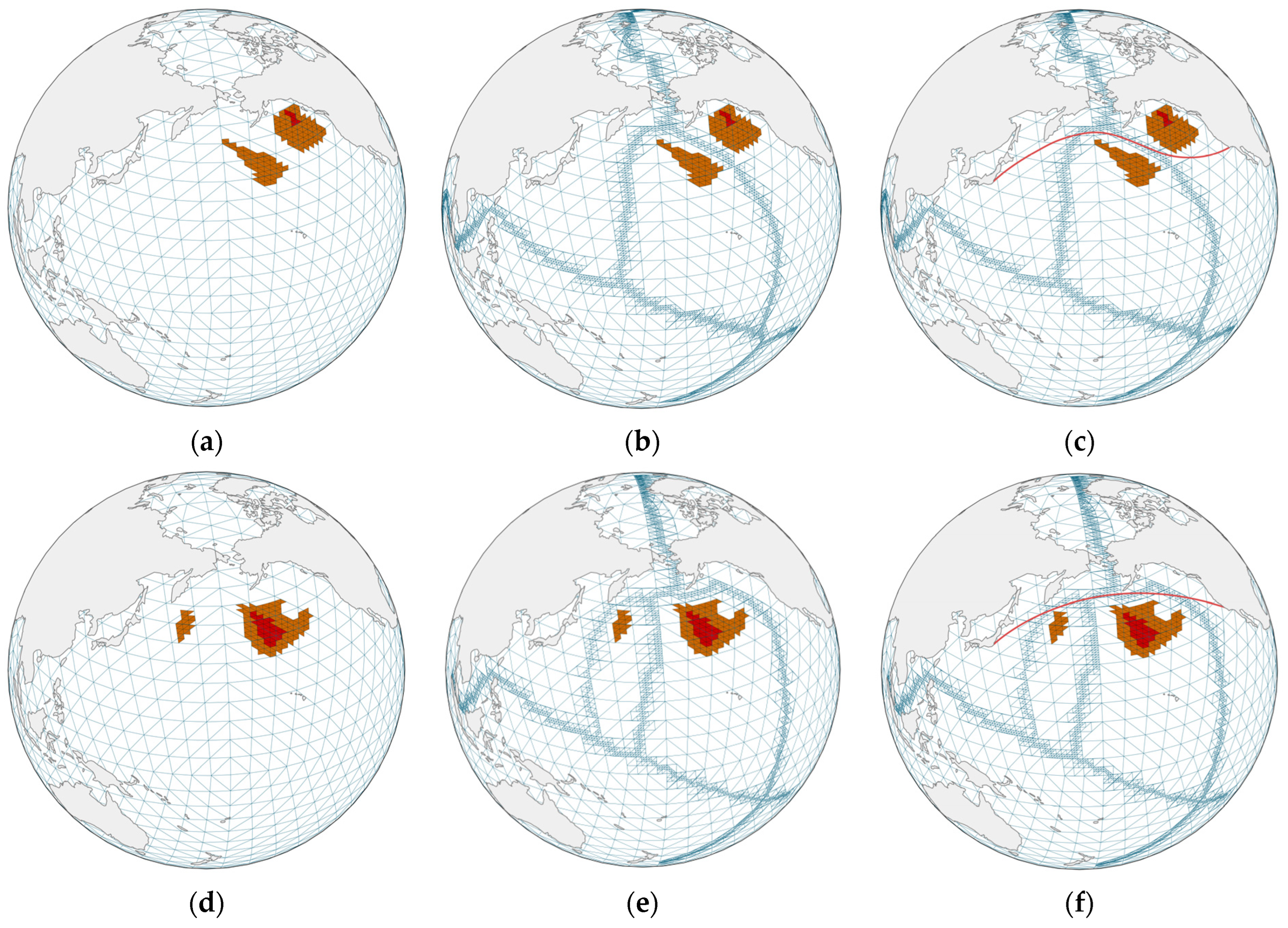
This paper employs a multi-level Quadrilateralized Triangular Mesh (QTM) as a framework for global data integration. Utilizing the sixth level of the QTM, with an approximate edge length of 200 km, the study incorporates authentic ocean storm wave height data sourced from the National Oceanic and Atmospheric Administration of the United States. Oceanic regions with wave heights exceeding 5 m are delineated by orange grids, while areas with waves over 9 m are represented by red grids, as illustrated in Figure 14a.

Figure 14.
Dynamic construction of Voronoi diagrams based on landmasses and storm areas, and ship routing. The orange-red area represents storm regions, gray represents landmasses, and red lines denote planned shipping routes.
Subsequently, the spherical Voronoi diagram is constructed using the land and storm regions as the generating surfaces, as depicted in Figure 14b. Thereafter, the A* algorithm is employed to derive safe routes that circumvent both land and storm areas, followed by the application of a polynomial interpolation method to smooth these paths, with the results presented in Figure 14c. Maritime weather conditions are subject to change, with significant alterations in the oceanic wind and wave hazard areas, as shown in Figure 14d, necessitating adjustments to the navigation paths of ocean vessels. Utilizing the spherical Voronoi diagram update algorithm presented in this paper, the Voronoi diagram is updated, with the outcomes displayed in Figure 14e. Subsequently, the ship’s path is adjusted accordingly, as depicted in Figure 14f.
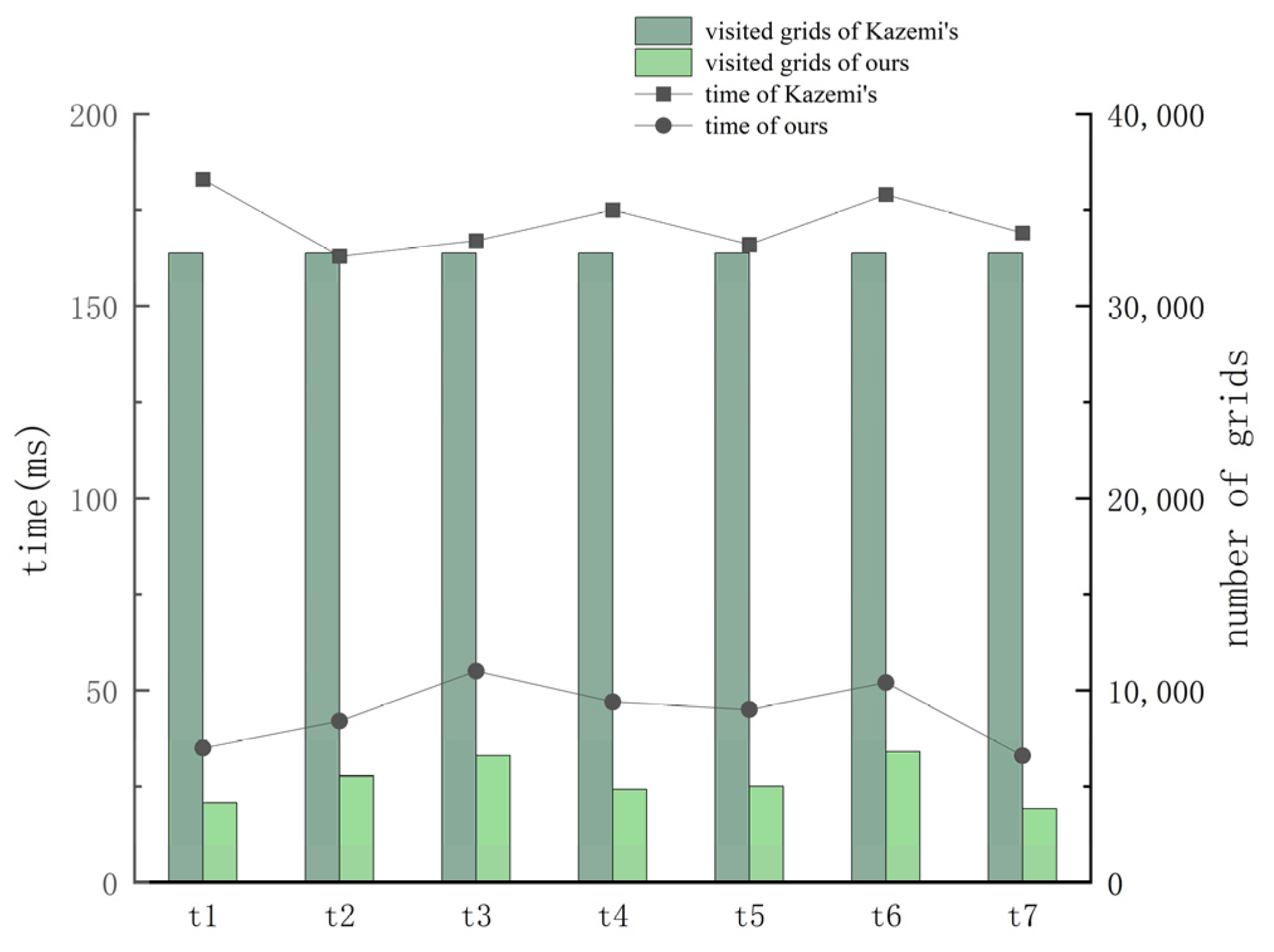
Figure 15 presents a comparative analysis of the number of grids accessed and the time required for the updates of spherical Voronoi diagrams over time between the algorithm introduced in this paper and Kazemi’s algorithm. Kazemi’s algorithm involves a complete reconstruction of the Voronoi diagram, resulting in an invariant number of grid accesses and a nearly constant time requirement. In contrast, our algorithm accesses a significantly smaller number of grids within the updated regions. This indicates that our algorithm offers improved efficiency under dynamic conditions.
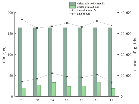
Figure 15.
Efficiency comparison of different algorithms in dynamic environments.
3.3.2. Global Vessel Management Based on Multi-Scale Voronoi Diagrams
This paper employs the 10th level of the QTM, with edges roughly 10 km in length, to integrate over 9000 global fishing vessel coordinates from Global Fishing Watch, constructing a global Voronoi diagram, as shown in Figure 16a. The Voronoi diagram delineates fishing resource areas for different vessels. Over time, the coordinates of approximately 500 vessels shifted, prompting updates to the Voronoi diagram. The outcomes of these updates are presented in Figure 16b, with the Voronoi regions corresponding to the altered vessels highlighted in green.
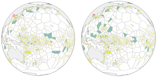
Figure 16.
Dynamic construction of Voronoi diagrams based on landmasses and vessels. The red box represents the area in the Figure 17 and altered vessels are highlighted in green.
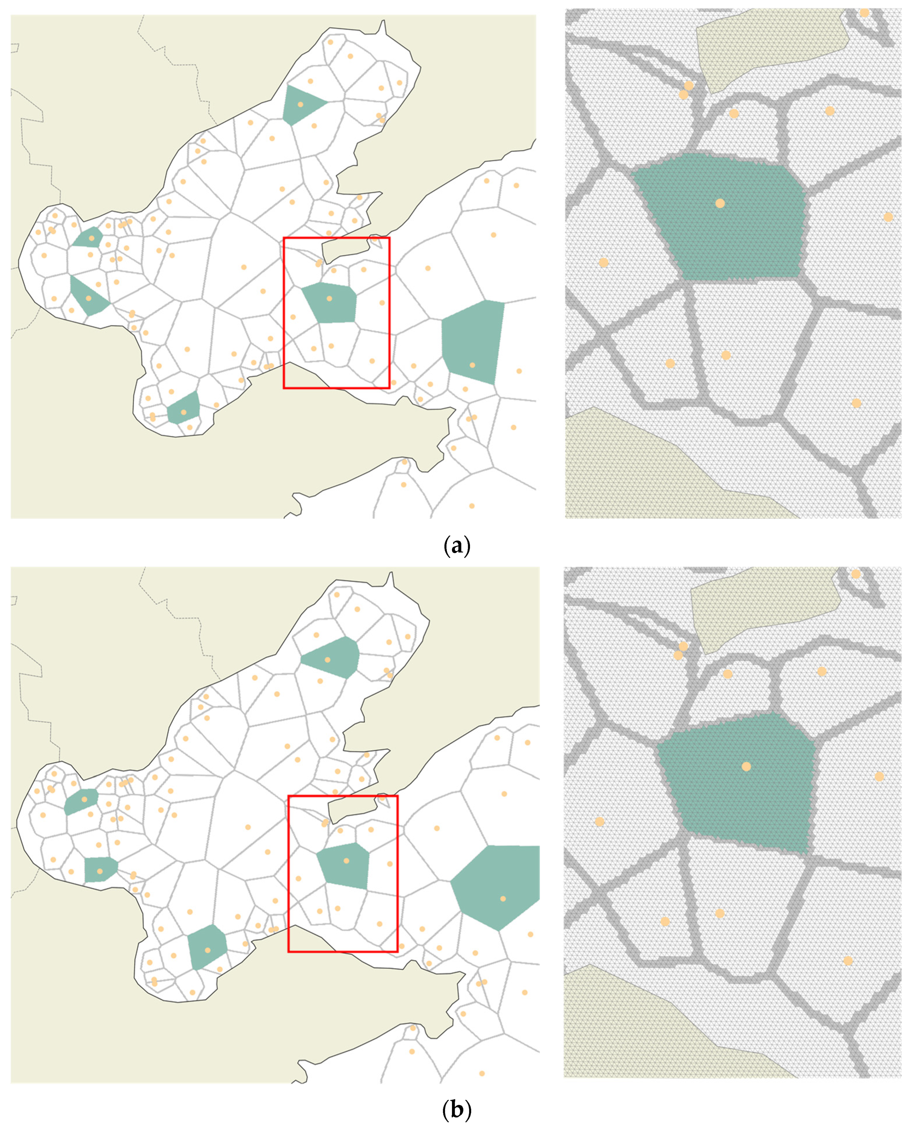
Within the context of a localized area, this study selects the Bohai Bay as the experimental region, based on the 14th level of the QTM, where the edge length of the grids is approximately 0.5 km. Figure 17 displays a grid-based Voronoi diagram constructed on a local scale within a globally unified framework, utilizing vessels and peninsulas as the generating elements. The positions of ships at sea change over time, and the updates to the Voronoi diagram are reflected in the results presented in Figure 17. An enlarged view on the right side of the figure highlights the changes in the grid-based Voronoi diagram following these updates.
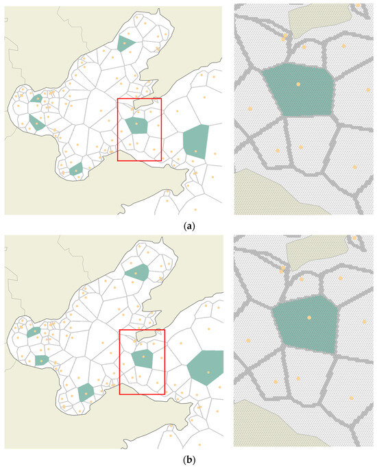
Figure 17.
Dynamic construction of Voronoi diagrams in a local area with higher resolution. The red box in the left figure represents the area in the right figure and altered vessels are highlighted in green.
In our global maritime dynamics management experiment, we constructed Voronoi diagrams at various scales. The environment incorporated static elements like landmasses and some ships, alongside dynamic factors such as storms and moving vessels, causing localized Voronoi diagram alterations over time. Our algorithm performs these updates locally rather than resorting to full reconstruction. Table 4 contrasts our approach with Kazemi’s algorithm in terms of the average update time and grid numbers across scales, demonstrating the superior efficiency of our method in the dynamic experiment.
Table 4.
Efficiency comparison of different algorithms for constructing Voronoi diagrams under dynamic environments.
It is noteworthy that beyond the application to ocean vessel management as covered in the experiments of this paper, spherical Voronoi diagram structures have found extensive application in significant domains such as airspace management and satellite planning. The algorithm presented in this paper has the potential to be extended to these fields, demonstrating a broad spectrum of application prospects.
4. Discussion
4.1. Spherical and Ellipsoidal Spatial Reference
Due to the distortions caused by projection and significant topological differences between the spherical and planar spaces [15], existing algorithms for updating planar space Voronoi diagrams [19,31,32,33,34,35] are not readily applicable to spherical space. Kazemi et al. [15] have experimentally demonstrated the superior accuracy of DGGS in performing spherical distance transformations compared to planar algorithms. Additionally, planar algorithms face challenges in processing at the Earth’s poles, as the singularity of the topological relationship at the poles also makes it difficult for planar algorithms to adapt. The Discrete Global Grid System (DGGS) is a global grid model based on the true geospatial space, which fits the Earth’s surface by recursively subdividing the spherical surface, thereby avoiding the various deformations and data fractures caused by planar projection. This paper, grounded in a spherical spatial reference, presents the design of Voronoi diagram generation and updating algorithms that are tailored to the characteristics of spherical grids, effectively resolving the aforementioned issues.
In the realms of geography and Earth science, to more effectively cater to the geospatial demands of the real world, numerous applications favor the use of a geodetic ellipsoid model—such as the WGS84 ellipsoid—over a basic spherical model as their foundational framework. These applications employ geodetic ellipsoidal distances as the standard measure, rather than spherical distances. The construction of vector Voronoi diagrams on an ellipsoidal surface is a complex task that necessitates iterative calculations based on the approximate coordinates derived from an auxiliary sphere [2]. For instance, Kastrisios et al. [6] constructed vector Voronoi diagrams on an ellipsoidal surface, where 17% of the vertices required iteration in excess of a hundred times.
The algorithm presented in this paper is applicable to both spherical and ellipsoidal spaces, contingent upon the underlying QTM framework employed. It may be predicated on a generic spherical model or aligned with an ellipsoidal model, with the distance metric selected being either spherical or ellipsoidal. The foundational triangles of the spherical QTM are constituted by spherical triangles with their vertices situated on the spherical surface. Conversely, the foundational triangles of the ellipsoidal QTM consist of ellipsoidal triangles with vertices positioned on the surface of the reference ellipsoid. This paper delineates the spherical distance benchmark and the ellipsoidal distance benchmark as the great-circle arc distance between the centroids of the spherical triangle grids or the ellipsoidal distance, respectively. For the computation of ellipsoidal distances, this paper adopts the WGS84 reference ellipsoid as the basis for the ellipsoidal model. The Python PYPROJ package, renowned for its robust ellipsoidal computation functions [36], is utilized, which is predicated on the classical Jacobi ellipsoidal functions; the ellipsoid is defined as
the ellipsoidal distance is defined as
Herein, (β, ω) represents the ellipsoidal latitude and longitude, and represents the path azimuth angle:
This paper leverages the PYPROJ toolkit to test the efficiency of distance calculations on spherical and ellipsoidal surfaces. The left axis of Figure 18 shows the time needed to compute distances 100,000 times. Subsequently, based on the eighth-level QTM tessellation, which includes approximately over half a million cells, Voronoi diagrams are constructed using both spherical and ellipsoidal distance metrics. The results are presented on the right axis of Figure 18. The experimental results indicate that the construction time for the ellipsoidal Voronoi diagram is slightly higher than that for the spherical Voronoi diagram, but it is still within an acceptable range.
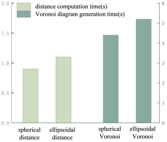
Figure 18.
Distance calculations and Voronoi diagram construction for spherical and ellipsoidal references.
This paper defines the distance metric as the spherical or ellipsoidal distance between the centroids of spherical triangular grids. The spherical distance is calculated based on the great-circle arc length, while the ellipsoidal distance is measured by the shortest path length over the reference ellipsoidal surface. The distance measurement within the grid space is not entirely equivalent to the point-to-point distance in vector space, and this process inevitably introduces some error. The results of the algorithm presented in this paper limit the error to within a single grid cell. The grid of QTM possesses attributes of multi-resolution and infinite subdivision. The average unit area and average edge length of the grids at different levels of the QTM, based on ellipsoidal and spherical benchmarks, are shown in Table 5. In practical applications, one can select the grid scale based on specific requirements, balancing the needs for efficiency and accuracy to control the error. For instance, in the experiments of Section 3.3, a global-scale route is approximated for ocean-going vessels, utilizing the sixth-level grid to establish a 20 km navigational interval for vessel transit. When allocating fishing resources for marine fishing boats, the 14th-level grid is chosen, with a grid edge length of approximately 500 m and a boundary error within 500 m. For detailed navigation and obstacle avoidance operations of the vessels, a higher-resolution grid can be delineated in the local area. If the requirement is to control the error within 10 m, the 20th-level grid can be selected.
Table 5.
Average side length and average area of grid based on spherical and ellipsoidal surfaces at different resolutions.
4.2. Voronoi Diagram Construction Based on Multi-Resolution Grids
In global spatial applications, there is a significant disparity in the scales of various applications and data. Spherical vector Voronoi diagrams face certain challenges when applied across multiple scales. This is due to the fact that vector data are typically stored as a collection of geometric elements such as points, lines, and polygons, each with specific positional and attribute information. When attempting to represent spatial information at different scales, the vector data structure may need to adapt by either subdividing or simplifying geometric elements, which can lead to an increase in data complexity and storage volume. This also augments the complexity of data processing and analysis.
In comparison, the QTM allows for infinite recursive subdivision to closely fit the Earth’s surface, with grids of varying resolutions nested within one another. The Voronoi diagrams constructed in this paper based on the QTM are inherently capable of adapting to geographic data from different sources and with different resolutions. The multi-level nature of the QTM provides a unified framework for Voronoi diagrams at various scales, enabling the integration and interaction of heterogeneous data and Voronoi diagrams with different resolutions within the same framework. This approach enhances the consistency and operability of the algorithms.
Taking Section 3.3 on ocean-going vessel navigation and management as an example, our approach balances efficiency and accuracy to generate Voronoi diagrams of varying resolutions based on application context. At a macro scale, we utilize continents and storm areas as generators to create high-resolution Voronoi diagrams for overall direction and route planning. In contrast, micro-scale local areas are addressed with finer resolution for more detailed boundary delineation.
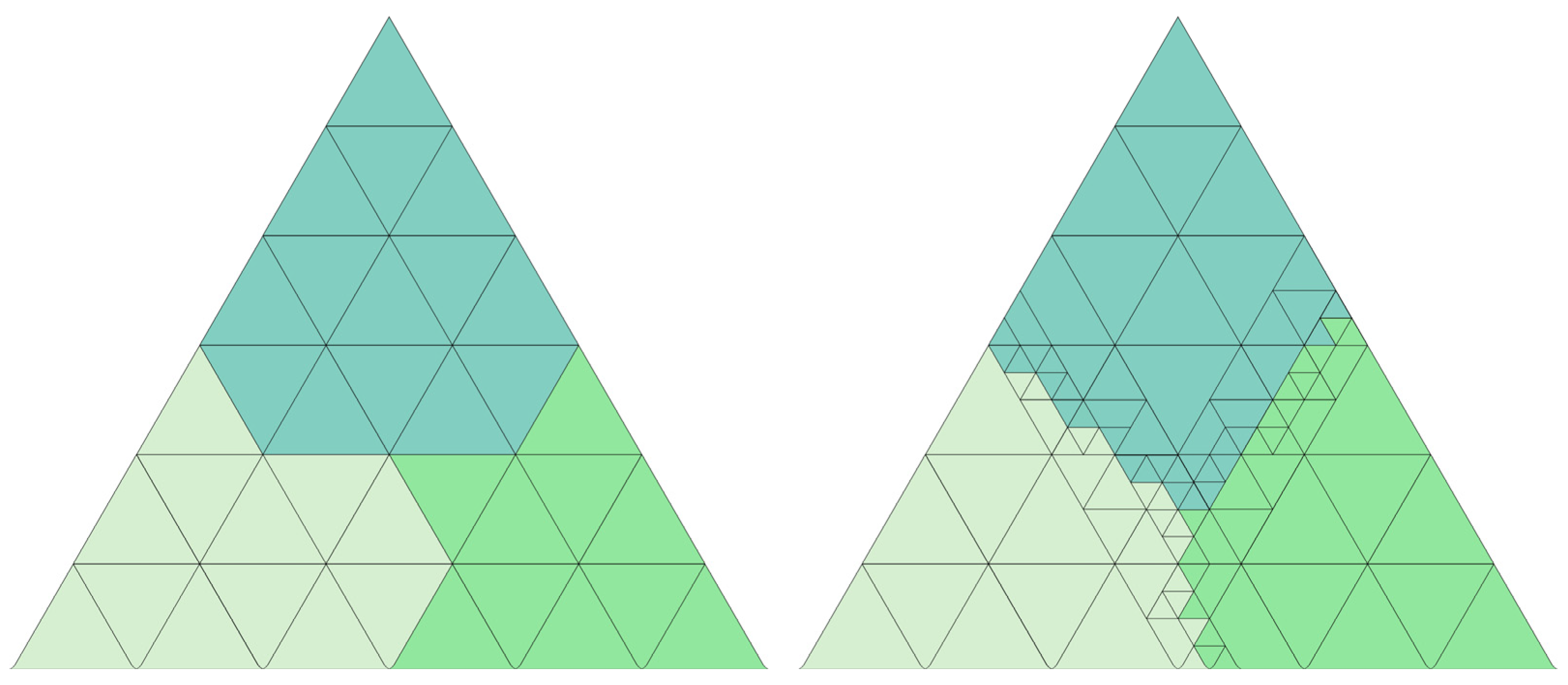
In the research presented in this paper, the transformation between Voronoi diagrams of different resolutions is achieved through the subdivision and merging of the Voronoi diagram’s boundary grids, as depicted in Figure 19. Specifically, when transitioning from a high-resolution Voronoi diagram to a lower-resolution one, the process begins with the subdivision of the boundary grids, yielding four smaller triangles. The subsequent goal is to determine the closest feature point to each of these four smaller triangles individually. Given that grids within the same Voronoi region are generally continuous, the four smaller triangles can each select the closest feature point from the nearest feature points of their parent grid and the neighboring grids of the parent grid. After calculating the distances to each of these points individually, the new boundary of the Voronoi region is established. Subsequently, the aforementioned process is repeated until the grid resolution of the Voronoi region boundary meets the desired target resolution. Conversely, the conversion from a low-resolution grid Voronoi diagram to a high-resolution grid is relatively straightforward. This is because the nearest feature point for the high-resolution grid can be derived from the feature point of the most central small triangle. This operation can be accomplished based on the hierarchical indexing of the grids.
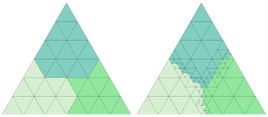
Figure 19.
Interconversion of Voronoi diagrams with different resolutions, with different colors indicating different Voronoi regions.
This study has achieved interconversion between Voronoi diagrams of different resolutions by the hierarchical characteristics of the QTM. However, the research has not fully utilized the multi-level features within the process of the Voronoi diagram update algorithm. Specifically, in this study, when dealing with high-resolution and low-resolution Voronoi diagrams, updates were performed independently for each, without fully integrating the update process for multi-scale Voronoi diagrams at the algorithmic level. This is due to the fact that we must consider the update frequency and the update areas of Voronoi diagrams at different scales. If we aim to establish a unified update process for multi-resolution Voronoi diagrams, we should fully consider the relationships between Voronoi diagrams of various scales, including the selection of the scale and direction for the dilation. For example, during an ordered dilation of the grid, one might choose to dilate by expanding 10 units of the 6th-level grid, 2 units of the 8th-level grid, and 1 unit of the 10th-level grid in the northeast direction. This approach helps to reduce computational redundancy and the need for redundant judgment when converting between different resolution Voronoi diagrams, thereby achieving consistency and efficiency in the global update of Voronoi diagrams. It allows the algorithm to be more flexible in adapting to the needs of different scales, which may potentially enhance the efficiency of the algorithm. We express a keen interest in further exploring this aspect and plan to focus on resolving this issue in our subsequent research.
4.3. Interoperability between Different Grids in Voronoi Diagrams
Global discrete grids are available in various fundamental shapes, with the shape of grid cells determining the storage, indexing, and relational characteristics of the grid system. Each type of partitioned grid possesses distinct structural advantages. A triangular grid offers high rendering efficiency and more accurate boundary fitting. A diamond-shaped grid can leverage the rich algorithms of planar grids. A hexagonal grid benefits from adjacency consistency. Since different grids are suitable for different application scenarios, to meet the application needs of various fields and to achieve the optimal expression, processing, and analysis of various types of global spatiotemporal data, there is a requirement for transformation between different grid models.
The global discrete grid system is constituted by “grid points”, “grid edges,” and “grid cells”. Grid points act as the central control elements of the DGGS, usually arranged at certain intervals across the Earth’s surface. Their density is contingent upon the selected grid system and its corresponding level of partitioning. Grid edges represent the boundaries or connectors between adjacent grid points, delineating the regional boundaries and the structural framework of the grid system. Grid cells are polygons formed by the grid edges surrounding adjacent grid points, with each grid cell signifying a spatial unit within the global discrete grid system. Grid points that share the same spatial distribution can create various grid cell systems through distinct arrangements of grid edges. There is potential to investigate a unified expression pattern from grid points to different grid cells.
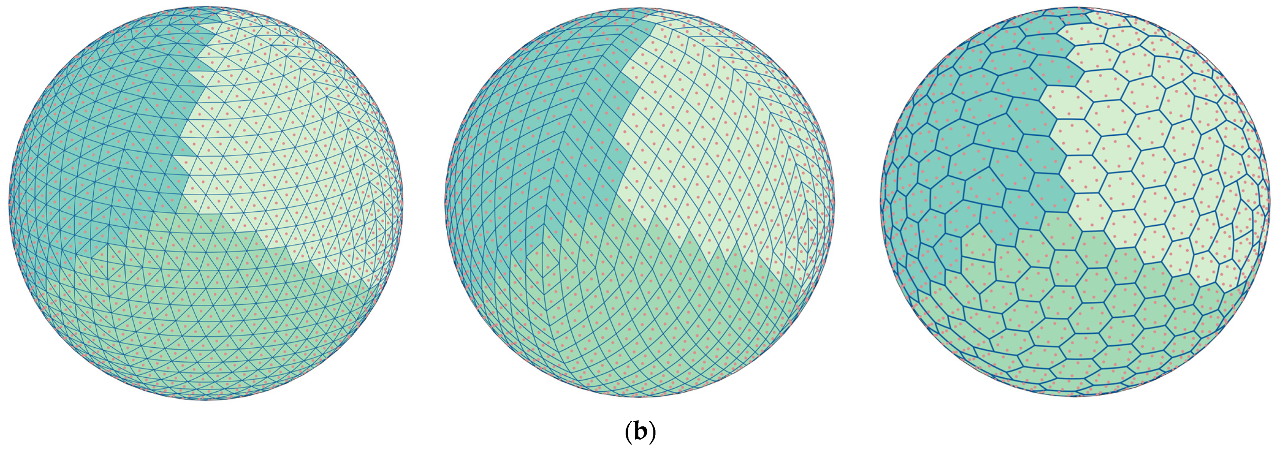
Based on this concept, we can develop a set of spherical Voronoi diagram construction and update models centered around grid points, independent of the shape of the grid cells. Specifically, using the centroids of octahedral QTM as grid points, we can construct isomorphic diamond-shaped and hexagonal grids. Each triangular grid encompasses a single grid point, while a diamond-shaped grid, which is composed of two triangular grids, encompasses two grid points. Furthermore, a hexagonal grid, consisting of six triangular grids, encompasses six grid points, as depicted in Figure 20a. Utilizing this unified model centered on grid points enables facile transformation between grid cells of diverse shapes.
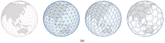
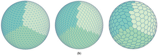
Figure 20.
Interoperability of Voronoi diagrams based on grid points. (a) Grid points; (b) Voronoi diagrams, with different colors indicating different Voronoi regions.
For raster spherical Voronoi diagrams, the Voronoi region attribute of each grid is determined by the proximity of the central point to the nearest feature point. The algorithm presented in this paper is capable of determining the nearest feature point for each grid point within a triangular grid. In diamond-shaped Voronoi diagrams, the grids are defined by the two internal grid points, whereas in hexagonal Voronoi diagrams, the grids are determined by the six internal grid points, as depicted in Figure 20b. Utilizing this method, the transformation between grids of different shapes based on the grid point system can be easily accomplished, thus meeting the needs of various application scenarios. It should be noted that this conversion process may lead to some information loss.
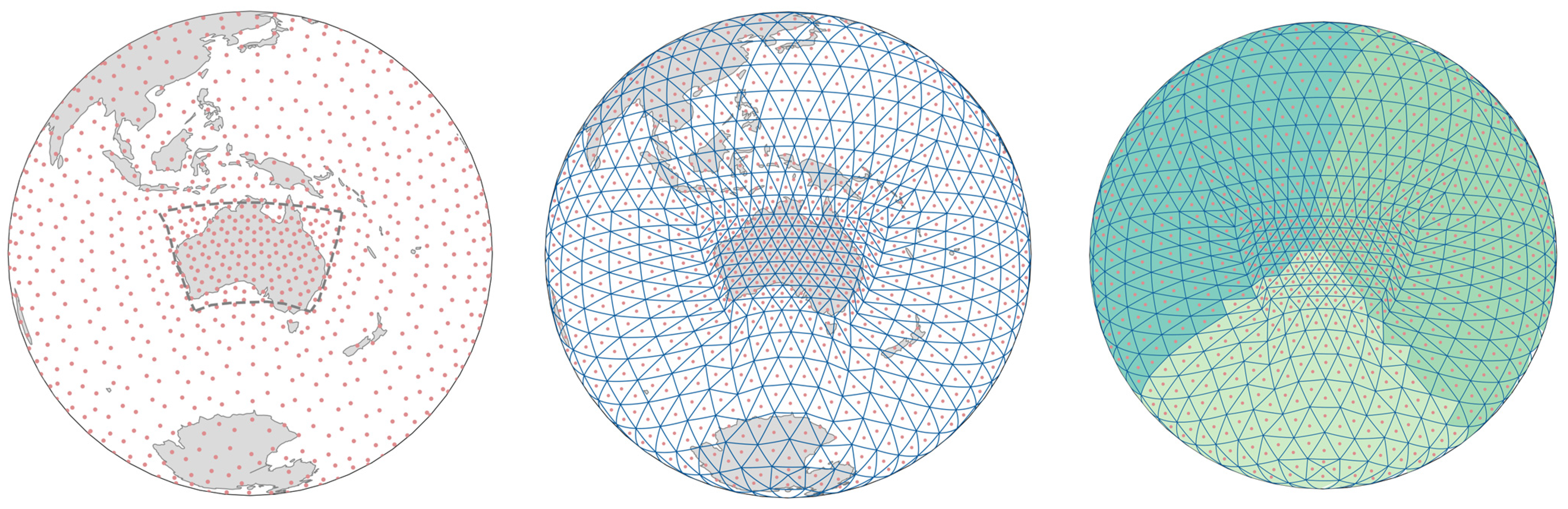
In conclusion, the construction of spherical Voronoi diagrams based on grid points offers the flexibility to adapt to various grid shapes and application backgrounds, along with high scalability and universality. Moreover, the mobility of grid points allows for a better fit to the data, thereby enhancing the accuracy of the model. As illustrated in Figure 21, grid points can be aggregated into areas of interest without altering the topological structure of the grid, which does not impact the application of the Voronoi diagram algorithm presented in this paper. This aggregation results in a denser Voronoi diagram in specific regions, effectively increasing the local resolution. Consequently, this approach enables a clearer acquisition of information from focal areas, facilitating a more in-depth analysis of the characteristics and variations within those regions.
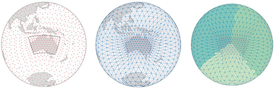
Figure 21.
Variable-resolution Voronoi diagrams. The red dots represent grid points, with different colors indicating different Voronoi regions.
The perturbation of grid points enables the construction of spherical Voronoi diagrams with variable resolutions. The unaltered topological relationships of the grid ensure the usability of the algorithm presented in this paper. However, the acceptable degree of perturbation requires further research. Perturbation can alter the distribution of grid points to a certain extent, and it is essential to ensure that such alterations do not adversely affect the accuracy and stability of the Voronoi diagram algorithm to an unacceptable degree. Therefore, additional experimental testing is necessary to determine the acceptable range of perturbation. Moreover, the multi-level of the grid point system is also worth exploring, implementing hierarchical subdivision based on the perturbed grid points and constructing spherical Voronoi diagrams on this foundation. This provides new perspectives and methodologies for the modeling and updating of Voronoi diagrams based on a global discrete grid.
5. Conclusions
In the realm of Earth science applications, spherical raster Voronoi diagrams are of considerable significance. The traditional generation algorithms of spherical raster Voronoi diagrams find it challenging to achieve precision and efficiency as well as to dynamically maintain the structure of the Voronoi diagrams. This study introduces a dynamic construction scheme for raster Voronoi diagrams based on the QTM, which is utilized for the generation, updating, and multi-scale visualization of spherical Voronoi diagrams. The main contributions are as follows:
- This paper designs a three-tier data structure, comprising dictionaries and queues, tailored to the attributes of spherical multi-level Voronoi diagrams and the characteristics of the algorithm.
- The canonical ordering strategy is introduced, a spherical ordered dilation algorithm is designed based on the properties of the spherical triangular grid, and a special treatment is designed for the topological structure of spherical grids.
- This paper presents our algorithm through pseudocode and conducts comparative experiments to evaluate its feasibility and efficiency. The experimental results indicate that when reconstructing the entire Voronoi diagram, the efficiency of our algorithm is comparable to that of other spherical grid algorithms; however, it demonstrates significant efficiency advantages when handling localized updates of the Voronoi diagram.
- Additionally, with the global dynamic navigation and management of ocean vessels as the application context, this paper designs and demonstrates the construction, updating, and visualization of spherical Voronoi diagrams at different scales, demonstrating the utility of the proposed algorithm.
In summary, the research findings contribute to the construction and updating of spherical Voronoi diagrams, offering broad potential in the global dynamic management applications. The next step involves extending the algorithm proposed to multiple scales and across various grid morphologies, followed by additional experimental testing and validation.
Author Contributions
Conceptualization, Qingping Liu and Xuesheng Zhao; methodology, Qingping Liu; software, Qingping Liu, Yuanzheng Duan and Mengmeng Qin; validation, Qingping Liu, Yuanzheng Duan and Mengmeng Qin; formal analysis, Qingping Liu and Mengmeng Qin; investigation, Qingping Liu and Yuanzheng Duan; resources, Mengmeng Qin and Wenlan Xie; data curation, Wenlan Xie; writing—original draft preparation, Qingping Liu; writing—review and editing, Qingping Liu and Xuesheng Zhao; visualization, Qingping Liu and Yuanzheng Duan; supervision, Xuesheng Zhao and Wenbin Sun; project administration, Qingping Liu; funding acquisition, Xuesheng Zhao and Wenbin Sun. All authors have read and agreed to the published version of the manuscript.
Funding
This research was supported by the general program of the National Natural Science Foundation of China [grant numbers 42371412 and 42271435].
Data Availability Statement
The meteorological data were sourced from the National Oceanic and Atmospheric Administration (NOAA) of the United States, which can be accessed at https://www.ndbc.noaa.gov/, accessed on 11 April 2024; the vessel data were retrieved from the non-profit organization Global Fishing Watch, available at https://globalfishingwatch.org/, accessed on 11 April 2024.
Acknowledgments
We would like to thank NOAA and Global Fishing Watch for providing data.
Conflicts of Interest
The authors declare no conflicts of interest.
Appendix A
| Algorithm A1: Partial pseudocode for the ordered dilation procedure |
| Input: dilationQueue: the queue of grids for the next dilation |
Output: QTMDict: the data Structure for Voronoi diagram on QTM
|
| Algorithm A2: Partial pseudocode for Voronoi diagram update procedure |
| insert() |
| Input: insertSites: the insert sites, QTMDict: the data Structure for Voronoi diagram on QTM |
Output: QTMDict: the data Structure for Voronoi diagram on QTM
|
| delete() |
| Input: ds: the delete element number of sites, QTMDict: the data Structure for storing attributes of Voronoi sites |
Output: QTMDict: the data Structure for storing attributes of Voronoi sites
|
References
- Dai, G.; Chen, X.; Wang, M.; Fernández, E.; Nguyen, T.N.; Reinelt, G. Analysis of satellite constellations for the continuous coverage of ground regions. J. Spacecr. Rockets 2017, 54, 1294–1303. [Google Scholar] [CrossRef]
- Zhang, J.; Chen, S.; Ning, P.; Zhang, X. An equidistance/equiratio method of maritime delimitation on the Earth ellipsoid. J. Sea Res. 2023, 191, 102322. [Google Scholar] [CrossRef]
- Hashemi Beni, L.; Mostafavi, M.A.; Pouliot, J.; Gavrilova, M. Toward 3D spatial dynamic field simulation within GIS using kinetic Voronoi diagram and Delaunay tetrahedralization. Int. J. Geogr. Inf. Sci. 2011, 25, 25–50. [Google Scholar] [CrossRef]
- Liu, Y.; Yang, T. Impact of Local Grid Refinements of Spherical Centroidal Voronoi Tessellations for Global Atmospheric Models. Commun. Comput. Phys. 2017, 21, 1310–1324. [Google Scholar] [CrossRef]
- Pang, M.Y.C.; Shi, W. Development of a process-based model for dynamic interaction in spatio-temporal GIS. GeoInformatica 2002, 6, 323–344. [Google Scholar] [CrossRef]
- Kastrisios, C.; Tsoulos, L. Voronoi tessellation on the ellipsoidal earth for vector data. Int. J. Geogr. Inf. Sci. 2018, 32, 1541–1557. [Google Scholar] [CrossRef]
- Jacobsen, D.; Gunzburger, M.; Ringler, T.; Burkardt, J.; Peterson, J. Parallel algorithms for planar and spherical Delaunay construction with an application to centroidal Voronoi tessellations. Geosci. Model Dev. 2013, 6, 1353–1365. [Google Scholar] [CrossRef]
- Na, H.-S.; Lee, C.-N.; Cheong, O. Voronoi diagrams on the sphere. Comput. Geom. 2002, 23, 183–194. [Google Scholar] [CrossRef]
- Zheng, X.; Ennis, R.; Richards, G.P.; Palffy-Muhoray, P. A Plane Sweep Algorithm for the Voronoi Tessellation of the Sphere. Electron.-Liq. Cryst. Commun. (e-LC) 2011, 1, 1–13. [Google Scholar]
- Sugihara, K. Laguerre Voronoi diagram on the sphere. J. Geom. Gr. 2002, 6, 69–81. [Google Scholar]
- Kabluchko, Z.; Thäle, C. The typical cell of a Voronoi tessellation on the sphere. Discret. Comput. Geom. 2021, 66, 1330–1350. [Google Scholar] [CrossRef]
- Chen, J.; Zhao, X.; Li, Z. An algorithm for the generation of Voronoi diagrams on the sphere based on QTM. Photogramm. Eng. Remote Sens. 2003, 69, 79–89. [Google Scholar] [CrossRef]
- Hojati, M.; Robertson, C.; Roberts, S.; Chaudhuri, C. GIScience research challenges for realizing discrete global grid systems as a Digital Earth. Big Earth Data 2022, 6, 358–379. [Google Scholar] [CrossRef]
- Hu, H.; Liu, X.H.; Hu, P. Voronoi diagram generation on the ellipsoidal earth. Comput. Geosci. 2014, 73, 81–87. [Google Scholar] [CrossRef]
- Kazemi, M.; Wecker, L.; Samavati, F. Efficient calculation of distance transform on discrete global grid systems. ISPRS Int. J. Geo-Inf. 2022, 11, 322. [Google Scholar] [CrossRef]
- Kant, G. Drawing planar graphs using the canonical ordering. Algorithmica 1996, 16, 4–32. [Google Scholar] [CrossRef]
- Harabor, D.; Botea, A. Breaking path symmetries on 4-connected grid maps. In Proceedings of the AAAI Conference on Artificial Intelligence and Interactive Digital Entertainment, Palo Alto, CA, USA, 11–13 October 2010; pp. 33–38. [Google Scholar]
- Sturtevant, N.R.; Rabin, S. Canonical Orderings on Grids. In Proceedings of the IJCAI, New York, NY, USA, 9–15 July 2016; pp. 683–689. [Google Scholar]
- Qin, L.; Hu, Y.; Yin, Q.; Zeng, J. Speed Optimization for Incremental Updating of Grid-Based Distance Maps. Appl. Sci. 2019, 9, 2029. [Google Scholar] [CrossRef]
- Deng, C.; Cheng, C.; Qu, T.; Li, S.; Chen, B. A Method for Managing ADS-B Data Based on a 4D Airspace-Temporal Grid (GeoSOT-AS). Aerospace 2023, 10, 217. [Google Scholar] [CrossRef]
- Zhai, W.; Tong, X.; Miao, S.; Cheng, C.; Ren, F. Collision detection for UAVs based on GeoSOT-3D grids. ISPRS Int. J. Geo-Inf. 2019, 8, 299. [Google Scholar] [CrossRef]
- Robertson, C.; Chaudhuri, C.; Hojati, M.; Roberts, S.A. An integrated environmental analytics system (IDEAS) based on a DGGS. ISPRS J. Photogramm. Remote Sens. 2020, 162, 214–228. [Google Scholar] [CrossRef]
- Rawson, A.; Sabeur, Z.; Brito, M. Intelligent geospatial maritime risk analytics using the Discrete Global Grid System. Big Earth Data 2022, 6, 294–322. [Google Scholar] [CrossRef]
- Li, M.; McGrath, H.; Stefanakis, E. Multi-resolution topographic analysis in hexagonal Discrete Global Grid Systems. Int. J. Appl. Earth Observ. Geoinf. 2022, 113, 102985. [Google Scholar] [CrossRef]
- Li, Y.; Zhao, X.; Sun, W.; Wang, G.; Luo, F.; Wang, Z.; Duan, Y. A GtoG Direct Coding Mapping Method for Multi-Type Global Discrete Grids Based on Space Filling Curves. ISPRS Int. J. Geo-Inf. 2022, 11, 595. [Google Scholar] [CrossRef]
- Dutton, G. Modeling locational uncertainty via hierarchical tessellation. In Accuracy of Spatial Databases; CRC Press: Boca Raton, FL, USA, 1989; pp. 125–140. [Google Scholar]
- Lin, B.; Zhou, L.; Xu, D.; Zhu, A.-X.; Lu, G. A discrete global grid system for earth system modeling. Int. J. Geogr. Inf. Sci. 2018, 32, 711–737. [Google Scholar] [CrossRef]
- Schoener, M.; Coyle, E.; Thompson, D. An anytime Visibility–Voronoi graph-search algorithm for generating robust and feasible unmanned surface vehicle paths. Auton. Robot. 2022, 46, 911–927. [Google Scholar] [CrossRef]
- Xiong, C.; Chen, D.; Lu, D.; Zeng, Z.; Lian, L. Path planning of multiple autonomous marine vehicles for adaptive sampling using Voronoi-based ant colony optimization. Robot. Auton. Syst. 2019, 115, 90–103. [Google Scholar] [CrossRef]
- Öztürk, Ü.; Akdağ, M.; Ayabakan, T. A review of path planning algorithms in maritime autonomous surface ships: Navigation safety perspective. Ocean Eng. 2022, 251, 111010. [Google Scholar] [CrossRef]
- Kalra, N.; Ferguson, D.; Stentz, A. Incremental reconstruction of generalized Voronoi diagrams on grids. Robot. Auton. Syst. 2009, 57, 123–128. [Google Scholar] [CrossRef]
- Lau, B.; Sprunk, C.; Burgard, W. Efficient grid-based spatial representations for robot navigation in dynamic environments. Robot. Auton. Syst. 2013, 61, 1116–1130. [Google Scholar] [CrossRef]
- Qin, L.; Yin, Q.; Zha, Y.; Peng, Y. Dynamic detection of topological information from grid-based generalized Voronoi diagrams. Math. Probl. Eng. 2013, 2013, 438576. [Google Scholar] [CrossRef]
- Yin, Q.; Qin, L.; Liu, X.; Zha, Y. Incremental construction of generalized Voronoi diagrams on pointerless quadtrees. Math. Probl. Eng. 2014, 2014, 456739. [Google Scholar] [CrossRef]
- Chen, Y.; Lai, S.; Cui, J.; Wang, B.; Chen, B.M. GPU-Accelerated Incremental Euclidean Distance Transform for Online Motion Planning of Mobile Robots. IEEE Robot. Autom. Lett. 2022, 7, 6894–6901. [Google Scholar] [CrossRef]
- Karney, C.F. Geodesics on an ellipsoid of revolution. arXiv 2011, arXiv:1102.1215. [Google Scholar]


Disclaimer/Publisher’s Note: The statements, opinions and data contained in all publications are solely those of the individual author(s) and contributor(s) and not of MDPI and/or the editor(s). MDPI and/or the editor(s) disclaim responsibility for any injury to people or property resulting from any ideas, methods, instructions or products referred to in the content. |
© 2024 by the authors. Licensee MDPI, Basel, Switzerland. This article is an open access article distributed under the terms and conditions of the Creative Commons Attribution (CC BY) license (https://creativecommons.org/licenses/by/4.0/).