Abstract
The shape pattern recognition of building footprints stands as a pivotal concern within GIS spatial cognition. In this study, we introduce a novel approach for the shape recognition of building footprints, leveraging t-distributed stochastic neighbor embedding (t-SNE) dimensionality reduction visualization. First, the Canonical Time Warping (CTW) algorithm is employed to gauge the shape similarity distance of building footprints. Subsequently, the t-SNE model is utilized to map the building footprints, featuring varying numbers of coordinate vertices, onto points within the Cartesian coordinate system. The shape similarity distance serves as the input to the t-SNE model for parameter optimization. Lastly, building footprint shapes are identified through the inherent clustering patterns of points using a Gaussian Mixture Model (GMM). Experimental results demonstrate the method’s robustness to the translation, rotation, scaling, and mirroring of geometric objects, while effectively measuring shape similarity between building footprints. Furthermore, diverse types of building footprints are discernible through natural clustering in low-dimensional spaces, aligning closely with human visual perception.
1. Introduction
Building footprints, a fundamental component of geographical data, play a pivotal role in cartography and embody the distinct cultural attributes of civilizations throughout history. Examples include the pyramids of ancient Egypt, the colosseums of ancient Rome, and the quadrangles of old Peking, each representing the unique architectural styles of its respective culture. Recognizing the shapes of building footprints holds increasing significance in Geographic Information Systems (GIS) applications, encompassing spatial cognition, spatial queries, spatial question answering (QA), cartographic generalization, and map updating [1].
Numerous studies have explored shape recognition within geospatial databases, facilitating inquiries into distribution patterns [2], the simplification of building footprints via template matching [3], and the assessment of data quality by measuring shape similarity against templates [4]. An effective model for recognizing building footprints can accurately convey characteristic spatial information. The process of shape recognition for building footprints involves two primary stages: quantitatively describing shape characteristics and establishing a measurement model for shape differences (or similarities) [5].
Pattern recognition, a cornerstone of computer vision, has seen various methodologies proposed, including Dynamic Programming (DP), Dynamic Time Warping (DTW), and Canonical Time Warping (CTW) [6,7,8]. DP techniques leverage contour point sequences to establish local correspondences between shapes for measuring shape dissimilarity. DTW algorithms align series instances by minimizing an objective distance function, often solved via DP. Numerous variations and extensions exist, such as weighted DTW [9], Fast-DTW [10], and vector quantization DTW [11]. However, DTW and its derivatives struggle to align multimodal data. CTW methods, employing Canonical Correlation Analysis (CCA) to extract features, align time-series signals of varying lengths using DTW. Widely used in gait sequence recognition and the temporal alignment of multiple sequences, CTW outperforms other DTW-based techniques [12].
While the coordinate sequence of vector building footprints resembles a time series, few studies have applied CTW to calculate the distances between polygon coordinate sequences. This study transforms 2D vector building footprints into 1D coordinate sequences and utilizes CTW to measure shape similarity distances. Additionally, a method based on t-distributed stochastic neighbor embedding (t-SNE) is employed to map high-dimensional building footprints onto low-dimensional points for shape recognition [13]. t-SNE, a nonlinear dimensionality reduction technique, replaces high-dimensional polygons with low-dimensional points and categorizes them by transforming them into matrices with pairwise similarity information. In contrast to existing methods, dimensionality reduction-based methods can maintain both the local and global structures of the original high-dimensional data by projecting it into a lower-dimensional space. These methods provide interpretable results for shape recognition, unlike deep learning-based methods that rely on training data. Additionally, some dimensionality reduction-based methods enable the measurement of shape similarity without the need for constructing complex shape descriptors, such as the CTW method. Therefore, this paper integrates the local and global structures of building footprints to recognize the building footprints at the visualization level, which directly utilizes polygon coordinate sequences for shape similarity measurement, eschewing complex shape descriptors, and employs t-SNE to cluster similar building footprints visually and intuitively.
The remainder of this paper is structured as follows: Section 2 provides a review of related works. Section 3 outlines the principles of building footprint recognition using the t-SNE algorithm. In Section 4, experiments are conducted, and the proposed method is analyzed using real data. Finally, Section 5 presents discussions and conclusions.
2. Related Works
Methods for shape pattern recognition can be categorized into two main groups: similarity-based and clustering-based techniques. The similarity-based approach typically involves two stages: the quantitative characterization of shape attributes and the assessment of similarity. Humans generally discern various shapes based on region, structure, and contour characteristics, which serve as the foundation for quantifying shapes [14]. Region-based methods, such as grid-based descriptors and moment-based techniques, utilize statistical data to represent shape region information [15,16]. Structure-based methods commonly employ skeleton features to convey geometric and topological structural details [17]. Contour-based methodologies, including Fourier descriptors [18], the chain code method [19], turning function [20], shape context [21], hierarchical models [22], and contour point distribution histograms [23], quantify shape attributes by delineating graphic contours. Region-based approaches are susceptible to noise and may lose contour details, making them suitable for shapes with simple boundaries. Structure-based methods entail complex processes for extracting structural information and are suitable for shapes with simple structures. Contour-based techniques require the design of shape descriptors and may lack accuracy in describing shapes. Most of these methods are sensitive to transformations such as rotation, scale, and translation, impeding direct application in shape similarity measurements.
Following the quantitative description of shape attributes, shape differences can be gauged through similarity or dissimilarity measures. A greater similarity corresponds to smaller distances. Statistical and shape attributes serve as common indicators for measuring building footprint similarity. Statistical characteristics like distance, direction, and geometric factors are frequently utilized [24]. Geometric coding, Fourier descriptors, and turning functions are prevalent shape attribute measurement techniques. Geometric coding methods compare coding similarity using simple calculation functions but are less accurate for complex shapes. Fourier descriptors represent shape contours via Fourier transform and measure similarity by comparing low-order coefficient differences. Turning functions represent the relationship between tangent angle and arc length, measuring similarity by tangent angle discrepancies. The conventional statistical features of polygons, such as area, perimeter, centroid, bounding rectangle, along with simple shape descriptors like geometric coding, Fourier descriptors, and turning functions, all struggle to adequately characterize the shape features of complex building footprint polygons. These complexities may encompass irregularities along the edges, variations in concave and convex sections, the presence of sharp angles, and unconventional contour shapes.
Recent advances in dimensionality reduction techniques have been leveraged for object and shape recognition. Dimensionality reduction maps high-dimensional input objects to lower-dimensional spaces, where similar attributes are clustered together [25]. These techniques are classified into linear and nonlinear reductions, with nonlinear methods prevalent due to the nonlinearity of real-world data. Local Binary Pattern (LBP), local directional patterns (LDP), and Maximum Variance Unfolding (MVU) are common nonlinear dimensionality reduction methods. For instance, LBP has been applied in face recognition [26], LDP in gender classification and object recognition [27,28], and t-distributed stochastic neighbor embedding in facial expression recognition [29] and eye movement pattern identification [30]. Additionally, a unique ship-handling behavior pattern has been recognized through t-SNE-based dimensionality reduction and visualization [31].
With the advancement of deep learning technology, neural networks have recently been employed in the field of map pattern recognition. Reference [32] presents a method for recognizing drainage patterns in river networks using a graph convolutional neural network. Meanwhile, reference [33] details a technique for the pattern recognition and segmentation of administrative boundaries, utilizing a one-dimensional convolutional neural network and grid shape context descriptor. However, the aforementioned methods are primarily focused on the pattern recognition of linear features in maps. Building footprints, characterized by artificial traces and typical right-angle features, necessitate the development of specialized methods for their shape pattern recognition. This study innovatively employs t-SNE to recognize building footprint shapes through intuitive point visualization in low-dimensional spaces. High-dimensional space distances are calculated using the CTW algorithm as shape similarity distances, with Gaussian Mixture Model (GMM) used for recognition accuracy assessment. The proposed method introduces a novel approach to shape similarity measurement and recognition within the GIS domain.
3. Methodology
The methodology for building footprint recognition is illustrated in Figure 1, encompassing three main stages: (1) Transformation of shapes into vector coordinate sequences, followed by a computation of the similarity distances between these sequences using the CTW algorithm. (2) Integration of the t-SNE algorithm to incorporate shape similarity distances as the matrix among high-dimensional data. After dimensionality reduction, vector representations of building footprints (in high dimension) are projected onto multiple point clusters (in low dimension), each cluster representing a distinct shape type. (3) Utilization of the GMM algorithm to evaluate recognition accuracy based on the inherent clustering patterns of points and actual building footprints. The shape recognition result is determined by the clustering category assigned to each building footprint.
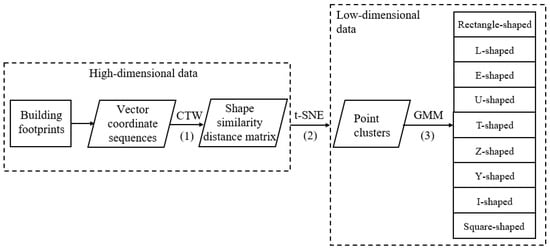
Figure 1.
The comprehensive flowchart outlining the recognition of building footprints using t-SNE.
Through this methodology, building footprints on a 2D plane are represented as 1D coordinate sequences. In process (1), the CTW algorithm enables the warping of one (or two) sequences by skipping several points within the local range to achieve optimal alignment. The distance obtained via the CTW algorithm serves as the shape similarity metric between building footprints, preserving invariance to translation, rotation, and scaling. In process (2), t-SNE utilizes a Gaussian distribution to transform the shape similarity among building polygons (in high-dimensional space) into a probability distribution. Subsequently, Student’s t-distribution is employed to convert distances into a probability distribution within point clusters (in low-dimensional space). The optimization of Kullback–Leibler divergence between these two distributions yields the dimensional reduction visualization. Buildings with similar shapes in high-dimensional space will approach each other and cluster together in the same point cluster in low-dimensional space. In contrast, buildings with significant differences in shape will repel each other in low-dimensional space and be separated into different categories of shape point groups. In process (3), the Gaussian Mixture Model (GMM) technique is employed to cluster and identify the reduced dimensional point clusters. Building polygon types are discerned based on the distribution of corresponding points. Detailed methodologies are elaborated upon in subsequent subsections.
3.1. Assessing the Shape Similarity of Building Footprints
The CTW algorithm calculates the canonical warping distance, which merges the DTW and CCA algorithms. Initially introduced for precise spatiotemporal alignment between two sequences [34]. Given two sequences, X = , Y = , CTW uses DTW to optimally align the sequences of X and Y that minimize the following sum-of-squares costs, as in:
where the warping path ( denotes the composition of alignment in frames, and refers to the number of indexes to align the two series. must satisfy the following constraints. Given and , (1) Boundary: , (2) Continuity: , and . (3) Monotonicity: and . Numerous warping paths meet the aforementioned conditions; nevertheless, the DTW algorithm exclusively extracts the shortest path utilizing the DP algorithm, as described in Equation (2).
where the cumulative distance is defined as the distance in the current cell, and the minimum cumulative distance of the adjacent elements. To integrate the CCA and DTW algorithms, Equation (1) can be reformulated in matrix notation, as depicted by Equation (3).
where and are two binary selection matrices that need to be inferred to align X and Y. Figure 2 shows an example of DTW for aligning the two series.
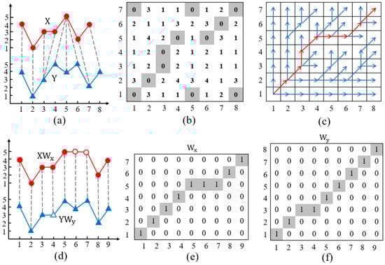
Figure 2.
An example DTW for aligning two series. (a) Two series (m = 7 and n = 8) and the optimal alignment between samples computed by DTW. (b) Euclidean distances between X and Y. (c) DP policy at each pair of samples, where the red curve donates the optimal warping path (K = 9). (d) A matrix-form interpretation of DTW as stretching the two sequences in matrix products. (e) Warping matrix . (f) Warping matrix .
Building upon the foundation of the DTW algorithm, CTW incorporates a linear transformation () akin to CCA. This transformation aims to identify the linear combination where the variables in X exhibit the highest correlation with those in Y, achieved by maximizing the expression presented in Equation (4).
After normalizing the sequences X and Y, the above equation can be reduced to , when and are replaced by the unit matrix due to the orthogonality constraint, Equation (4) can be transformed into the subsequent optimization model, subject to constraints, represented as Equation (5).
Equation (5) allows for the determination of the optimal linear transformation coefficients and of the original sequences X and Y based on Singular Value Decomposition. Given that and can be interpreted as the projection matrices of two sequences, they remain invariant to translation, rotation, and scaling. The CTW algorithm integrates DTW and CCA by minimizing Equation (6).
where and determine the spatial warping by projecting the sequences into the same coordinate system, and warp the sequences to achieve the optimum alignment. Similar to CCA, we also need to impose the following constraints: (1) , ; (2) ; and (3) is a diagonal matrix, where is a K identity matrix, , , . The algorithm begins by initializing and with identity matrices, and the canonical warping distance can be obtained by iteratively computing until the algorithm converges.
Nevertheless, the canonical warping distance is susceptible to variations in the starting point and direction of the coordinate sequences. To address this, we uniformly generated vector coordinate sequences in a clockwise direction and adjusted the starting point position based on the coordinate sequence. This adjustment ensures the derivation of the minimum value of CTW(X,Y) between X and Y, serving as the ultimate shape similarity distance [3]. The calculation procedure for CTW is illustrated in Figure 3.
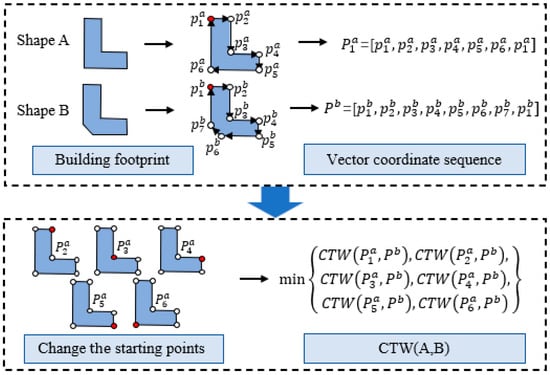
Figure 3.
The intricate procedure delineating shape similarity measurement via CTW.
(1) Given two building footprints marked as A and B, suppose A has n vertices, B has m vertices, and and are the starting points of A and B. The vector coordinate sequence, of A can be described as , and the vector coordinate sequence, of B can be described as . . is the coordinate of point in A. , is the coordinate of point in B.
(2) Select different vertices in A as the starting point and generate a set of sequences in the clockwise direction, which are represented as . where is the coordinate sequence that starts at the vertex in A. Subsequently, the canonical warping distance between the sequences in and , denoted as the minimum, serves as the ultimate distance between A and B, as depicted by Equation (7).
where the smaller the , the higher the shape similarity between those two shapes.
Figure 4 shows an L-shaped building (A) and its shapes after translation (B), scaling (C), and rotation (D). Table 1 lists the canonical warping distance matrix between A, B, C, and D at different starting points. As shown in Table 1, the canonical warping distances between A and the three transformed shapes are almost equal to 0 when is the starting point, which indicates that these four shapes are very similar, and the shape similarity calculated by the CTW method is in accordance with human visual cognition. The experimental results showed that the CTW algorithm is suitable for measuring the similarity of building footprints.
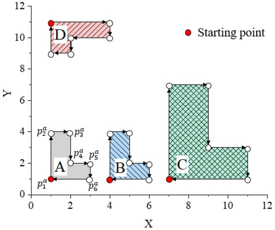
Figure 4.
L-shaped template (A) and the shapes after translation (B), scaling (C), and rotation (D).

Table 1.
The canonical warping distance between four shapes in Figure 4 at different starting points.
3.2. Express the Shape Similarity of Building Footprints by t-SNE
The main idea of the t-SNE algorithm is to reduce high-dimensional data to a lower-dimensional space while maintaining the probability between them. Denoting X = {, , , } as the d-dimensional input dataset, and Y = {, , , } as the embedding of X in the s-dimensional space, where s is much smaller than d, commonly s = 2 or 3. The t-SNE algorithm aims to find a low-dimensional data representation Y that minimizes the mismatch between and , which is achieved by minimizing the following Kullback–Leibler divergence that measures the difference between two probability distributions, as in:
where C is the cost function [13], P and Q are matrices of , and their elements are and , respectively. is the joint probability between and in high dimensions and is defined as Equation (9).
where is the variance of the Gaussian that is centered over each high-dimensional datapoint , which needs to be binary searched by a fixed perplexity to obtain the best. The perplexity is defined by Equation (10).
where is the joint probability between and in low dimensions and is defined as Equation (11).
As shown in Equation (12), the t-SNE method employs a gradient-based technique to minimize the Kullback–Leibler divergence between and . The gradient descent method is shown in Equation (13), where is the solution at iteration , indicates the learning rate, and (t) represents the momentum factor at iteration .
Figure 5 illustrates the detailed process of the proposed method for building footprint recognition. Diverging from the conventional t-SNE algorithm, our approach converts the Euclidean distance (as in Equation (9)) between high-dimensional data points into shape similarity distance. Here, high-dimensional data pertains to the data at the high-dimensional feature level, specifically the shape of the building polygon. The shape similarity distance determines the probability of the high-dimensional data points (building polygons) selecting each other as neighbors under a Gaussian distribution. As depicted in Figure 5, when the similarity between two building footprints is high, they are positioned close to each other in a low-dimensional space (point cluster). Conversely, if the similarity is very low, they are distantly separated from each other.
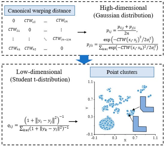
Figure 5.
The elaborate process of recognizing building shapes utilizing the t-SNE algorithm.
Hence, the joint probability between two building footprints can be expressed as Equation (14).
In low-dimensional space, similar types of building footprints aggregate to form clusters, while dissimilar building footprints repel each other. This results in a low-dimensional representation that mirrors pairwise similarity, such as the canonical warping distance, in the input representation. By examining the distribution of building polygons mapped within point clusters—whether closely concentrated within clusters or scattered outside— the specific building shape corresponding to each point can be discerned. Through visualization, our method enables the direct recognition of the shape of building polygons.
3.3. Recognize the Building Footprints by GMM
GMM serves as a valuable tool for data clustering, positing that all data points are linear combinations of finite Gaussian distributions [35]. In our investigation, the GMM technique was employed for point cluster recognition. Mathematically, GMM is expressed as a parametric probability density function and can be formulated as Equation (15).
where is a set of input data and is the probability that the input data belong to the component of the mixture, . is the average and is a covariance matrix, which can be full, diagonal, or spherical. is the number of sub-Gaussian models in the mixture model. represents the probability density function of the component, which can be defined as Equation (16).
Here, μ denotes the set of mean vectors, Σ represents the set of covariance matrices, and signifies the dimension of the input object.
4. Experiments and Analysis
4.1. Datasets
The experimental dataset was sourced from vector buildings at a scale of 1:10,000 in Wuhan, China, as depicted in Figure 6. This dataset comprised 742 building polygons. The residential buildings within the study area exhibited typical characteristics common to urban structures. Nine template shapes were manually created based on this dataset, including rectangular, L-shaped, E-shaped, U-shaped, T-shaped, Z-shaped, Y-shaped, I-shaped, and square-shaped buildings. As outlined in Table 2, the highest number of buildings in the study area were rectangular, followed by square-shaped buildings, while the lowest counts were observed for Y-shaped buildings, with E-shaped buildings following closely behind.
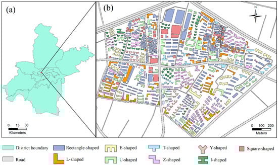
Figure 6.
Study area and dataset: (a) Wuhan region, and (b) the experimental dataset.
Table 2.
Statistics for the experimental dataset.
We utilized the Canonical Warping Distance function in Mathematica 12.1 to compute the similarity distance between building footprints. Subsequently, we developed the proposed method to visualize the 742 polygons using Python.
4.2. Recognition of Building Footprints and Analysis
We utilized the canonical warping distance among the 742 shapes depicted in Figure 6 as the similarity distance and applied the t-SNE algorithm to visualize the polygons into point clusters. As illustrated in Figure 7, Figure 8 and Figure 9, a series of experiments were conducted with varied initial values of iteration, learning rate, and perplexity to examine the impact of multiple parameters on building footprint recognition. In order to measure the accuracy of the t-SNE algorithm under different parameters, this paper used the GMM algorithm to cluster these points, and represented the clustering results with red dashed circles, each representing the same shape category identified by the t-SNE algorithm. The accuracy of shape recognition can be measured by comparing the clustering results of the points inside the circle with the actual shape they represent.
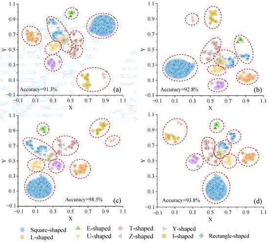
Figure 7.
The visualization of different values of iteration (a) 500, (b) 1000, (c) 1500, (d) 2000 with 800 learning rate and 30 perplexity value.
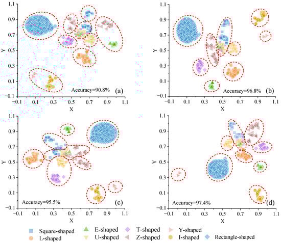
Figure 8.
The visualization of different learning rates (a) 200, (b) 400, (c) 600, (d) 1000 with 30 perplexity value and 1500 iterations.
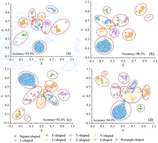
Figure 9.
The visualization of different perplexity (a) 10, (b) 30, (c) 50, (d) 70 with 800 learning rate and 1500 iterations.
It is important to note that the distance between different clusters in two-dimensional space does not necessarily reflect the similarity between different types of shapes. For instance, in Figure 7a, the clusters of U-shaped and square-shaped points appear closer together; however, this proximity does not imply a higher similarity between U-shaped and square-shaped buildings. Upon running the t-SNE algorithm multiple times based on the same experimental data, different distribution patterns of point clusters may emerge. Sometimes, U-shaped and square-shaped clusters are relatively distant from each other, while at other times, they may be closer.
A comparison of the visualization results in Figure 7 and Figure 8 reveals that the relative distribution patterns of the points remain largely consistent across different values of iteration and learning rate. Conversely, the point distributions in Figure 9, with varying perplexity values, exhibit noticeable discrepancies. This suggests that our method’s outcomes are relatively insensitive to iterations and learning rates but are significantly influenced by the perplexity parameter. Consequently, the subsequent sections focus on exploring the impact of different perplexity values on visualization results.
As depicted in Figure 9, under consistent iterations and learning rate settings but varying perplexity values, the 742 building footprints exhibit a distribution pattern where similar data points are drawn together while dissimilar ones repel each other. Previous research [13] has suggested that perplexity can serve as an indicator of the smoothness of the number of effective neighbors. An optimal perplexity value can be empirically determined through multiple visualizations with different perplexity values, with the best result being selected based on the quality of visualization.
Our experiments reveal that smaller perplexity values preserve more local structure, resulting in more compact clusters with greater diversity in cluster categories. Conversely, larger perplexity values preserve more global structure, leading to greater sparsity within clustered samples and increased separation between clusters. For instance, Figure 9a exhibits a compact distribution with relatively low perplexity. Here, square- and Y-shaped clusters are inaccurately divided into two sub-clusters, with insignificant separation between other clusters. Overlapping phenomena between clusters, such as partial point groups of square shapes, Z-shapes, and U-shapes, are observed.
Figure 9b–d demonstrate that as perplexity values increase, differences between shapes within the same category are magnified, and the distribution of data points within the same cluster becomes more dispersed. Notably, in Figure 9d, E-shapes and I-shapes retain more global structures.
In terms of clustering accuracy, Figure 9b outperforms those with perplexity values of 10, 50, and 70. Furthermore, regarding the separation of each cluster, Figure 9b surpasses Figure 9a,c,d. Hence, subsequent research will concentrate on analyzing the visualization results from Figure 9b, which was generated with 1500 iterations, 800 learning rates, and a perplexity value of 30.
Table 3 illustrates the accuracy of the proposed method in recognizing different shape types in Figure 9b using the GMM technique. Here, N0 represents the count of the shapes consistent with human cognition after clustering with the GMM method, while N1 represents the count of incorrectly classified shapes. Table 3 demonstrates that 98.5% of shapes were accurately clustered. Specifically, all the building footprints of rectangles, T-shaped, Y-shaped, I-shaped, and squares were correctly clustered. However, the accuracy of E-shaped buildings is the lowest (only 89.3%). On the one hand, this is because E-shaped buildings are the most complex in the experimental data, and their boundary contours are composed of multiple irregular parts. The complexity makes it difficult for the algorithm to accurately capture the similarity between these shapes. On the other hand, the sample size of E-shaped buildings in this experiment is the smallest, accounting for 3.77%, which results in low accuracy. Overall, the experimental results showcase the excellent separation of point clusters in low-dimensional space, validating the feasibility of our method for shape recognition.
Table 3.
The accuracy for recognizing different types of shapes with 1500 iterations, 800 learning rates and 30 perplexity values by GMM method.
In Figure 10a, the points enclosed within each red ellipse denote buildings classified as the same type using the GMM method. Notably, several other building types are erroneously classified as square shapes. Figure 10b illustrates the identification outcomes specifically for square shapes attained through the GMM clustering approach. We highlight all misclassified buildings, where “misclassified” also encompasses deviations from the shapes of other building types.
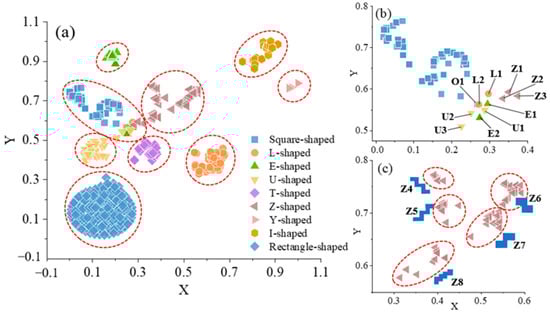
Figure 10.
(a) Shapes clustered by GMM, (b) Square-shapes, (c) Z-shapes.
In investigating the deviation of these 11 shapes depicted in Figure 10b, we conducted calculations to determine the canonical warping distance between these shapes and nine fundamental templates. The outcomes are presented in Table 4, wherein O1 indicates the deviation of the square shapes, while the remaining shapes are inaccurately clustered. Notably, shapes L2, E2, Z1, and Z3 are misidentified as square-shaped, I-shaped, Y-shaped, and L-shaped, respectively. These shapes deviate from the typical characteristics of their respective categories. Specifically, shape L2 exhibits ambiguity, rendering it susceptible to being cartographically generalized as square shapes in small-scale maps. Shapes E2, Z1, and Z3 are intricate polygons with irregular distortion and deformation relative to E- and Z-shaped templates, resulting in erroneous identification.
Table 4.
Shape similarity distance between the template and the deviated shapes.
When vertically comparing the data in Table 4, it becomes apparent that the distances between the deviated shapes and the templates are considerably larger than the average distance between correctly clustered shapes and the templates. Most of these distances exceed three times the standard deviation, resulting in the presence of “outliers” points. Take L-shapes as an example: the average distance between L-shapes and the template is 0.45, with a standard deviation of 0.57. However, the distance between shape L1 and the L-shaped template is 2.5, exceeding both the average distance and three times the standard deviation. Consequently, shape L1 is erroneously clustered in low-dimensional space and becomes an outlier. Conversely, compared to the other eight templates, the distance between shape L2 and the L-shaped template is the smallest, allowing the “outliers” shape L2 to still be correctly recognized.
This phenomenon can be attributed to two factors. Firstly, the t-SNE algorithm is symmetric. In asymmetric scenarios where the calculations of conditional probability and Kullback–Leibler divergence are asymmetric, the data points within each cluster will not select outliers as their neighbors. However, in symmetric scenarios, outliers choose the points in the nearest cluster, thereby shortening the distance between the outliers and other clusters. Secondly, the t-SNE algorithm employs a Gaussian distribution to calculate joint probability in high-dimensional space, while utilizing the Student’s t-distribution with one degree of freedom to calculate joint probability in low-dimensional space. The heavier tails of the Student’s t-distribution compared to the Gaussian distribution cause discrepancies in the probabilities between high- and low-dimensional spaces, leading to larger representations of the distances between data points in low-dimensional space. Consequently, similar shapes are closely distributed, while diverse shapes are dispersed outside clusters in low-dimensional space.
When horizontally comparing the data in Table 4, the presence of “outliers” is influenced by both the proposed algorithm and the characteristics of shape structures. Shape recognition is subjective, relying on human cognition shaped by cultural backgrounds, intentional interests, and emotions. Different individuals may recognize the same shape differently. For instance, some may identify shape U1 in Table 4 as a U shape, while others may perceive it as an L shape. Similarly, shape L2 may be recognized as either a square or an L shape by different individuals. Moreover, uncertainty in shape recognition may cause the same shape to be identified as other templates. For example, the canonical warping distance between shape U1 and the U-shaped template is 2.4, while the distance between shape U1 and the L-shaped template is 2.8, indicating close distances between the “outliers” and ambiguous templates.
Therefore, “outliers” in point clusters can reflect ambiguous shapes, and the distribution of points (in low-dimensional space) after dimension reduction by our method is closely related to corresponding shape structure characteristics (in high-dimensional space).
Furthermore, the results demonstrate that the proposed method effectively visualizes the shape of high-dimensional polygons as low-dimensional point clusters while preserving both local and global structural characteristics. For the global structures of building footprints, our method can successfully separate nine different types of shapes. Regarding local structures, Z-shaped buildings are further subdivided into several different shapes, as shown in Figure 10c, shapes Z4-Z8. Among these five types of shapes, Z4 and Z5, Z6, and Z7 are mirror images of each other, with shapes Z4 and Z5 represent third-order Z templates, and shape Z8 represents a fourth-order Z template. This indicates that the CTW algorithm is not only invariant to translation, rotation, and scaling, but also to mirroring.
Regarding time consumption, the proposed method exhibits an algorithmic complexity of O(N3), where N represents the number of points comprising the shape contour. Notably, the time cost of the algorithm escalates with an increase in the vertices of a polygon.
5. Conclusions
In this research, we present an innovative approach for recognizing building footprints utilizing t-SNE dimensionality reduction visualization. Our study makes several significant contributions:
- Utilization of the CTW Algorithm for shape similarity measurement: We creatively employ the CTW algorithm to measure the shape similarity distance of buildings. This approach remains invariant to translation, rotation, scaling, and mirroring in the mathematical model. By directly measuring the shape similarity distance of polygons using vector coordinate sequences, without the need for constructing complex encodings or shape contour descriptors, our method demonstrates the enhanced alignment of geometry vector sequences and an improved operability for building footprint similarity measurements.
- Innovative use of t-SNE algorithm for shape recognition: We creatively employ the t-SNE algorithm for shape recognition, converting the Euclidean distance between high-dimensional data points into shape similarity distance. Building footprints are then recognized based on the natural clustering results of points using the GMM method. As a nonlinear dimensionality reduction method, t-SNE enables the recognition of building footprints at the visualization level, offering greater intuitiveness and visibility compared to other shape recognition methods, such as SQL spatial query and template matching.
- Furthermore, our method efficiently categorizes buildings without label information by visualizing them, along with labeled buildings, into point clusters. The shape type of the point cluster to which unclassified buildings belong serves as the final recognition result. Our approach not only extracts shape characteristics but also retains local and global structures by producing clusters with reasonable separation. This enables a more efficient visualization of geospatial shapes with high-dimensional attribute characteristics in a low-dimensional space.
It is important to note that our proposed method may struggle to correctly measure the shape similarity distance of complex polygons twisted and deformed on a template basis and polygons with multiple regions. To address the limitations of the CTW algorithm in handling building footprints with complex structures, traditional shape simplification methods can be integrated with the CTW algorithm. This combination enhances the algorithm’s robustness and accuracy. Regarding the sensitivity of the t-SNE algorithm to parameters, incorporating deep learning or other machine learning techniques can facilitate the automatic selection of optimal parameters. Future research will focus on improving this method for the shape recognition of high-resolution remote sensing data and other geographical features, such as rivers and road networks.
Author Contributions
Conceptualization, Jingzhong Li; Methodology, Jingzhong Li; Software, Kainan Mao; Validation, Kainan Mao; Resources, Kainan Mao; Data curation, Kainan Mao; Writing—review and editing, Jingzhong Li; Visualization, Kainan Mao; Supervision, Kainan Mao; Project administration, Jingzhong Li. All authors have read and agreed to the published version of the manuscript.
Funding
This work was financially supported by the National Natural Science Foundation of China (Grant number 42271454 and 42394063); the Graduate Education Teaching Quality Improvement Project of Lanzhou Jiaotong University under Grant JG202301; the Natural Science Foundation of Hubei Province (Grant number 2022CFB053); and the Open Fund of Key Laboratory of Urban Land Resources Monitoring and Simulation, Ministry of Natural Resources (Grant number KF-2022-07-017).
Data Availability Statement
The data that support the findings of this study are openly available at https://doi.org/10.6084/m9.figshare.22360567 (accessed on 6 May 2024). The python code for the t-SNE algorithm is available at the link: http://doi.org/10.6084/m9.figshare.24995468 (accessed on 6 May 2024).
Acknowledgments
We acknowledge any support not covered by the author’s contributions or funding sections, including administrative and technical support that is not covered and data materials for experiments.
Conflicts of Interest
The authors declare no conflicts of interest.
References
- Matikainen, L.; Hyyppä, J.; Ahokas, E.; Markelin, L.; Kaartinen, H. Automatic detection of buildings and changes in buildings for updating of maps. Remote Sens. 2010, 2, 1217–1248. [Google Scholar] [CrossRef]
- Shirani, K.; Solhi, S.; Pasandi, M. Automatic Landform Recognition, Extraction, and Classification using Kernel Pattern Modeling. J. Geovis. Spat. Anal. 2023, 7, 2. [Google Scholar] [CrossRef]
- Yu, W.; Ai, T.; Liu, P.; Cheng, X. The analysis and measurement of building patterns using texton co-occurrence matrices. Int. J. Geogr. Inf. Sci. 2017, 31, 1079–1100. [Google Scholar] [CrossRef]
- Xu, Y.; Xie, Z.; Chen, Z.; Wu, L. Shape similarity measurement model for holed polygons based on position graphs and Fourier descriptors. Int. J. Geogr. Inf. Sci. 2016, 31, 253–279. [Google Scholar] [CrossRef]
- Yan, X.; Ai, T.; Yang, M.; Tong, X. Graph convolutional autoencoder model for the shape coding and cognition of buildings in maps. Int. J. Geogr. Inf. Sci. 2021, 35, 490–512. [Google Scholar] [CrossRef]
- Guo, H.; Liu, X.; Song, L. Dynamic programming approach for segmentation of multivariate time series. Stoch. Environ. Res. Risk Assess. 2015, 29, 265–273. [Google Scholar] [CrossRef]
- Jain, B. Making the dynamic time warping distance warping-invariant. Pattern Recognit. 2019, 94, 35–52. [Google Scholar] [CrossRef]
- Zhou, F.; Torre, F. Canonical time warping for alignment of human behavior. In Proceedings of the 22nd International Conference on Neural Information Processing Systems, Vancouver, BC, Canada, 7–10 December 2009; Curran Associates Inc.: Red Hook, NY, USA, 2009; pp. 2286–2294. [Google Scholar]
- Jeong, Y.; Jeong, M.; Omitaomu, O. Weighted dynamic time warping for time series classification. Pattern Recognit. 2011, 44, 2231–2240. [Google Scholar] [CrossRef]
- Salvadora, S.; Chan, P. Toward accurate dynamic time warping in linear time and space. Intell. Data Anal. 2007, 11, 561–580. [Google Scholar] [CrossRef]
- Faundez-Zanuy, M. On-line signature recognition based on VQ-DTW. Pattern Recognit. 2007, 40, 981–992. [Google Scholar] [CrossRef]
- Xiao, Q.; Liu, S. Motion retrieval based on Dynamic Bayesian Network and Canonical Time Warping. Soft Comput. 2017, 21, 267–280. [Google Scholar] [CrossRef]
- Laurens, V.; Hinton, G. Visualizing Data using t-SNE. J. Mach. Learn. Res. 2008, 9, 2579–2605. [Google Scholar]
- Zhang, D.; Guo, L. Review of shape representation and description techniques. Pattern Recognit. 2004, 37, 1–19. [Google Scholar] [CrossRef]
- Lu, G.; Sajjanhar, A. Region-based shape representation and similarity measure suitable for content-based image retrieval. Multimed. Syst. 1999, 7, 165–174. [Google Scholar] [CrossRef]
- Fu, Z.; Fan, L.; Yu, Z.; Zhou, K. A Moment-Based Shape Similarity Measurement for Areal Entities in Geographical Vector Data. ISPRS Int. J. Geo-Inf. 2018, 7, 208. [Google Scholar] [CrossRef]
- Bai, X.; Yang, X.; Yu, D.; Latecki, L. Skeleton-based shape classification using path similarity. Int. J. Pattern Recognit. Artif. Intell. 2008, 22, 733–746. [Google Scholar] [CrossRef]
- Ai, T.; Cheng, X.; Liu, P.; Yang, M. A shape analysis and template matching of building features by the Fourier transform method. Comput. Environ. Urban Syst. 2013, 41, 219–233. [Google Scholar] [CrossRef]
- Cortelazzo, G.; Mian, G.; Vezzi, G.; Zamperoni, P. Trademark Shapes Description by String-Matching Techniques. Pattern Recognit. 1994, 27, 1005–1018. [Google Scholar] [CrossRef]
- Xu, Y.; Xie, Z.; Chen, Z.; Xie, M. Measuring the similarity between multipolygons using convex hulls and position graphs. Int. J. Geogr. Inf. Sci. 2020, 35, 847–868. [Google Scholar] [CrossRef]
- Daliri, M.; Torre, V. Robust symbolic representation for shape recognition. Pattern Recognit. 2008, 41, 1782–1798. [Google Scholar] [CrossRef]
- Chen, Z.; Zhu, R.; Xie, Z.; Wu, L. Hierarchical Model for the Similarity Measurement of a Complex Holed-Region Entity Scene. ISPRS Int. J. Geo-Inf. 2017, 6, 388. [Google Scholar] [CrossRef]
- Shu, X.; Wu, X. A novel contour descriptor for 2D shape matching and its application to image retrieval. Image Vis. Comput. 2011, 29, 286–294. [Google Scholar] [CrossRef]
- Ding, H.; Guo, Q.; Du, X. Measurement of similarity for spatial directions between areal objects. Geo-Spat. Inf. Sci. 2004, 7, 225–230. [Google Scholar] [CrossRef][Green Version]
- Velliangiri, S.; Alagumuthukrishnan, S.; Thankumar joseph, S. A Review on Dimensionality Reduction Techniques for Efficient Computation. Procedia Comput. Sci. 2020, 165, 104–111. [Google Scholar] [CrossRef]
- Ahonen, T.; Hadid, A.; Pietikäinen, M. Face description with local binary patterns: Application to face recognition. IEEE Trans Pattern Anal. Mach. Intell. 2006, 28, 2037–2041. [Google Scholar] [CrossRef]
- Jabid, T.; Kabir, M.; Chae, O. Gender Classification Using Local Directional Pattern (LDP). In Proceedings of the 2010 20th International Conference on Pattern Recognition, Istanbul, Turkey, 23–26 August 2010; pp. 2162–2165. [Google Scholar] [CrossRef]
- Jabid, T.; Kabir, M.; Chae, O. Local Directional Pattern (LDP)—A Robust Image Descriptor for Object Recognition. In Proceedings of the 2010 7th IEEE International Conference on Advanced Video and Signal Based Surveillance, Boston, MA, USA, 29 August–1 September 2010; pp. 482–487. [Google Scholar] [CrossRef]
- Yi, J.; Mao, X.; Xue, Y.; Compare, A. Facial Expression Recognition Based on t-SNE and AdaboostM2. In Proceedings of the 2013 IEEE International Conference on Green Computing and Communications and IEEE Internet of Things and IEEE Cyber, Physical and Social Computing, Beijing, China, 20–23 August 2013; pp. 1744–1749. [Google Scholar] [CrossRef]
- Burch, M. Identifying Similar Eye Movement Patterns with t-SNE. In Proceedings of the International Symposium on Vision, Modeling, and Visualization, Stuttgart, Germany, 10–12 October 2018; pp. 111–118. [Google Scholar]
- Gao, M.; Shi, G. Ship-handling behavior pattern recognition using AIS sub-trajectory clustering analysis based on the T-SNE and spectral clustering algorithms. Ocean Eng. 2020, 205, 106919. [Google Scholar] [CrossRef]
- Yang, M.; Huang, H.; Zhang, Y.; Yan, X. Pattern Recognition and Segmentation of Administrative Boundaries Using a One-Dimensional Convolutional Neural Network and Grid Shape Context Descriptor. ISPRS Int. J. Geo-Inf. 2022, 11, 461. [Google Scholar] [CrossRef]
- Xu, X.; Liu, P.; Guo, M. Drainage Pattern Recognition of River Network Based on Graph Convolutional Neural Network. ISPRS Int. J. Geo-Inf. 2023, 12, 253. [Google Scholar] [CrossRef]
- Zhou, F.; De la Torre, F. Generalized Canonical Time Warping. IEEE Trans. Pattern Anal. Mach. Intell. 2016, 38, 279–294. [Google Scholar] [CrossRef]
- Ahani, A.; Nadoushani, S.; Moridi, A. Regionalization of watersheds by finite mixture models. J. Hydrol. 2020, 583, 124620. [Google Scholar] [CrossRef]


Disclaimer/Publisher’s Note: The statements, opinions and data contained in all publications are solely those of the individual author(s) and contributor(s) and not of MDPI and/or the editor(s). MDPI and/or the editor(s) disclaim responsibility for any injury to people or property resulting from any ideas, methods, instructions or products referred to in the content. |
© 2024 by the authors. Licensee MDPI, Basel, Switzerland. This article is an open access article distributed under the terms and conditions of the Creative Commons Attribution (CC BY) license (https://creativecommons.org/licenses/by/4.0/).