Abstract
Numerous studies have examined land surface temperature (LST) changes in Thailand using remote sensing, but there has been little research on LST variations within urban land use zones. This study addressed this gap by analyzing summer LST changes in land use zoning (LUZ) blocks in the 2012 Chiang Mai Comprehensive Plan and their relationship with surface biophysical parameters (NDVI, NDBI, MNDWI). The approach integrated detailed zoning data with remote sensing for granular LST analysis. Correlation and stepwise regression analyses (SRA) revealed that NDBI significantly impacted LST in most block types, while NDVI and MNDWI also influenced LST, particularly in 2023. The findings demonstrated the complexity of LST dynamics across various LUZs in Chiang Mai, with SRA results explaining 45.7% to 53.2% of summer LST variations over three years. To enhance the urban environment, adaptive planning strategies for different block categories were developed and will be considered in the upcoming revision of the Chiang Mai Comprehensive Plan. This research offers a new method to monitor the urban heat island phenomenon at the block level, providing valuable insights for adaptive urban planning.
1. Introduction
In the past few decades, the acceleration of urbanization has been a consequence of the increasing urban population (according to the United Nations [1]), especially in cities in Southeast Asia, such as Thailand [2]. Urbanization rapidly transforms rural land into urban areas [3,4]. The modification of surface attributes, vertical expansion, and population growth modify the energy balance and microclimate, causing environmental issues [5]. Urbanization gives rise to the urban heat island (UHI) phenomenon, resulting in elevated temperatures within urban areas relative to the surrounding suburban or rural areas [6,7]. As Southeast Asia has undergone urbanization and industrialization, the extent and intensity of the UHI effect have increased [8,9]. The occurrences of UHIs have become more complex and diverse in terms of types and scale. This has an increasingly significant impact on regional climate change [10], energy consumption [11,12], environmental quality [13,14], and public health [15,16]. Addressing the impacts of UHIs is a primary concern in many research domains. UHIs are divided into atmospheric heat islands (AHIs) and surface urban heat islands (SUHIs). AHIs use meteorological data, ground observations, and numerical simulations, while SUHIs use land surface temperature (LST) measured via thermal infrared (TIR) remote sensing [2,4,10]. This method provides accurate thermal radiation data of urban surfaces through satellite technology. Our study used remotely sensed LST to depict the urban thermal environment, leveraging its benefits of quick data acquisition, wide coverage, and low cost, as highlighted in previous research [17,18,19].
Concerning urban areas, which constitute highly intricate environmental systems with distinct contexts in each city, the spatiotemporal characteristics of surface biophysical features emerge as pivotal elements in city landscapes and substantial contributors to the SUHI effect. One of the most complex research questions involves identifying the primary driving factor behind the SUHI. Extensive research has been conducted on the entrepreneurial impacts of LST from various perspectives [20,21]. Numerous studies have demonstrated the effective selection of spectral indicators for surface composition based on four key principles and rules: theoretical significance, practical ubiquity, ease of accessibility, and minimal redundancy. Researchers have opted for spectral indices like the normalized difference built-up index (NDBI), normalized difference vegetation index (NDVI), and modified normalized difference water body index (MNDWI) due to their effective ability to capture surface biophysical features and establish strong correlations with LST. This has been demonstrated in recent studies by Hu et al. [17] and Yao et al. [20]. Research has demonstrated that alterations in land use and land cover have a substantial impact on the intensity of the SUHI in various spatiotemporal scenarios [22]. Li et al. [23] found that rapid urbanization causes the integration of functions within built-up areas, resulting in the spatial heterogeneity of LST patterns. However, comprehensive studies exploring the interrelationships between the urban surface biophysics layer as well as landscape composition and overheating are still lacking in the developing regions of the tropics due to the challenges in obtaining accurate information on urban morphology at fine scales [24,25]. This study aims to bridge the knowledge gap regarding the effects of urban characteristics on SUHIs in tropical cities. Specifically, it analyzes the relationship between surface biophysical features and the thermal environment in urban land use planning, particularly in tropical Asia, with a focus on a city in Thailand. In several studies on the thermal environmental patterns and intra-urban thermal properties of Thailand, urban block schemes have been developed for finer segmentation of urban areas into varied types of units (e.g., administrative boundaries [26], urban functional zones [8,27], local climate zones [28], urban morphological blocks [29]) to characterize the heterogeneous thermal behavior of intra-city LSTs. For SUHI analysis of land use zoning plans, we came across a study by Keeratikasikorn and Bonafoni [30] which assessed the intensity of SUHIs within various land use zoning categories of the comprehensive land use zoning plan of Bangkok 2013 (B.E.2556). This study was conducted to identify SUHI intensity within the different land use zones. Different kinds of urban zones have varied climatic contexts and surface properties, leading to their distinct urban thermal behavior. While the thermal regimes and SUHI patterns have been well studied in large cities like Bangkok, less attention has been given to secondary cities in Thailand that are also affected. The current zoning schemes tend to focus more on surface structures and covers, and there is insufficient examination of spectral indicators for surface composition in land use zoning plans. As a result, this research aims to achieve two objectives: (1) to determine the impacts of urban surface biophysical parameters on LST variation in different urbanized zones and (2) to analyze the degree of response of the above relationship to the land use zoning blocks scale.
To account for the uncertainties introduced by the LST driving analysis, it is necessary to conduct a multifactorial investigation rather than focusing solely on unilateral driving effects. Therefore, understanding the combined driving effects of urban surface temperature variation is vital to UHI mitigation [17,20]. Several statistical methods have been used in previous research to identify the main driving factors influencing urban LST. However, due to the various spatiotemporal characteristics of LST, it has been challenging to determine the most dominant factors. Some of the commonly used methods are ordinary least-squares regression analysis [31,32], stepwise multiple linear regression [18,33], Pearson correlation analysis [33,34,35], and principal component analysis [36,37], all based on linear and normal distribution hypotheses. In this study, we used Pearson correlation analysis and stepwise regression. These methods allowed us to identify the significant predictors of LST without including all possible variables. We also employed popular methods to determine the relative contribution of spectral indices derived from multispectral remote sensing images to block-scale LST and its summer variation. At the urban functional block scale, which is also the basic unit of urban planning used to specify the planning controls for a block of land under regulations governing land use and development, there is widespread acknowledgment that vegetation characteristics, built-up surface factors, and hydrothermal features exhibit significant variations across these land use zoning blocks [9,30,38]. At present, there are limited works of literature that provide a comprehensive characterization of the multifactorial effects of LST variations, particularly at the scale of land use zoning blocks [17,18,20]. This study focuses on the impact of surface biophysical features and urban land use functions on LST from the perspective of land use planning. Through a case study of Chiang Mai, we assessed the impact of three potential driving factors on summer LST within the land use zoning (LUZ) blocks outlined in the Chiang Mai Comprehensive Plan 2012. The study proposes practical strategies for sustainable urban planning and management in Chiang Mai to mitigate the urban heat island effect.
2. Materials and Methods
2.1. Study Area
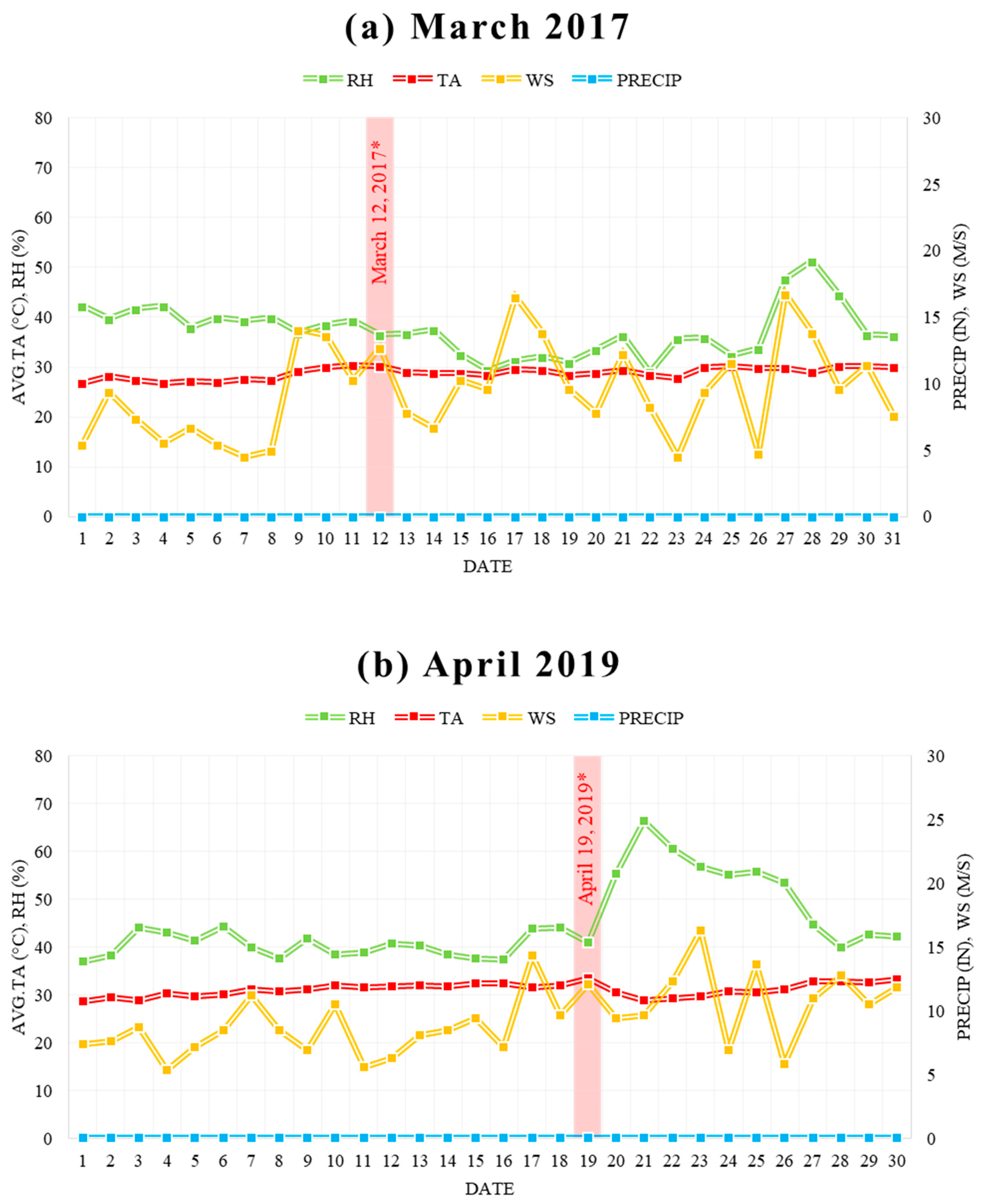
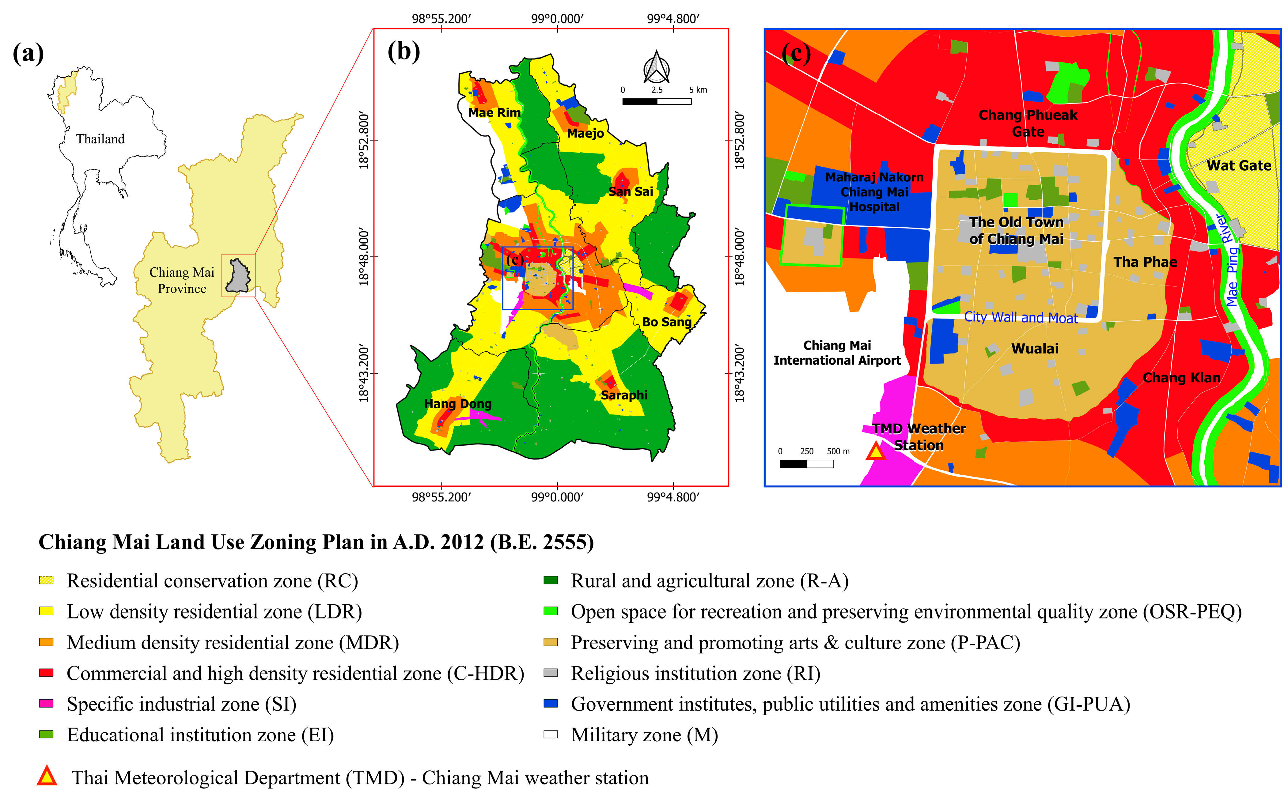
The city of Chiang Mai (98°59′07″ E, 18°47′18″ N), located in northern Thailand, serves as the major city of the north region (Figure 1a). The city experiences a tropical savanna climate, classified as type Aw by the Köppen climate classification [39]. The summer season, which is hot and humid, starts in early March and continues through late May. The Department of Public Works and Town and Country Planning (DPT) developed a revised land use zoning plan for Chiang Mai in accordance with the Town Planning Act B.E. 2518 (A.D.1975). This was done during the third comprehensive plan revision B.E. 2555 (A.D.2012), and the Chiang Mai Comprehensive Planning Act was officially registered in the government gazette after being signed by the Deputy of the Ministry of Interior. The approval became effective on 20 May 2013 and was valid for five years, from 2013 to 2017, with an additional two-year extension until 2019. Then, the Thai government passed the Town Planning Act B.E. 2562 (A.D. 2019), which aimed to improve urban development controls and focus on increasing participation from all sectors to promote inclusive and transparent urban planning. For this reason, there has been a delay in announcing its enforcement for the 4th revision of the Chiang Mai Comprehensive Plan until now. The enforcement of the 3rd revision of the land use plan has been ongoing since its development in 2012.
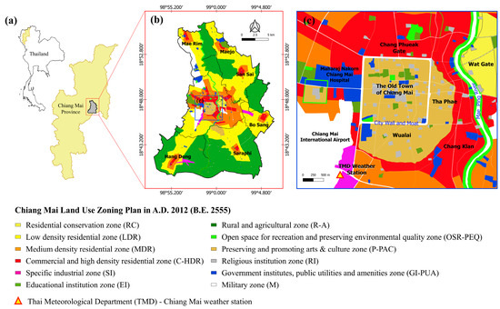
Figure 1.
Displays the location of the study area (a) and the land use zoning of Chiang Mai Comprehensive Plan 2012 (B.E. 2555) in Thailand (b,c).
The main goal of this plan was to address land use conflicts and the imbalanced development between urban and rural areas in Chiang Mai. This plan covered an area of about 430 square kilometers and included 12 zones; residential and development zones still make up the majority (50.43%). This is further divided into the low-density residential (LDR) zone (35.36%), the medium-density residential (MDR) zone (10.76%), the commercial and high-density residential (C-HDR) zone (3.72%), and the residential conservation (RC) zone (0.59%). Approximately 37.55% of the land use zoning plan is designated as rural and agricultural (R-A) zone to primarily protect the land for agricultural use (see Figure 1b,c and Table 1).

Table 1.
Chiang Mai’s 2012 Comprehensive Plan boundary includes data on the area and percentage of land use zonings (LUZs).
Rapid highway construction initiatives ensued after Chiang Mai’s economic growth, contributing to ongoing urban expansion [40]. Our findings indicate that these developments, particularly the creation of superhighways and the widening of radial roads, have led to significant changes in LST due to increased built-up areas. For example, our analysis shows higher LST values in areas near newly constructed highways and intersections, corroborating the findings of McGrath et al. [41] regarding spontaneous high-density development at these junctions. The expansion into rural properties and unplanned urban centers has exacerbated social and environmental issues, including the UHI effect. Our study highlights how poorly planned land use has resulted in built-up areas encroaching on previously arable land, further increasing LSTs in these regions. This aligns with our findings that show higher NDBI values correlate with increased LSTs, particularly in zones experiencing rapid urban sprawl. In Chiang Mai’s urban planning system, LUZ blocks play a crucial role in comprehensive planning, essential for analyzing changes in the urban microclimate and local ecosystems. Our research utilized these LUZ blocks to assess the impact of various biophysical parameters (NDVI, NDBI, MNDWI) on LST variations. The road network’s topological processing and block boundaries, based on major road distances and administrative sub-district maps, allowed us to pinpoint areas most affected by urban sprawl and its associated LST changes.
2.2. Datasets
Remote sensing images from Landsat 8 were obtained from the website of the United States Geological Survey (USGS), accessed on 28 April 2023 at http://earthexplorer.usgs.gov/. The Landsat 8 satellite has two sensors—the Operational Land Imager (OLI) for capturing land images and the Thermal Infrared Sensor (TIRS) for retrieving land surface temperature (LST). Surface temperatures vary more than atmospheric air temperatures during the day, but they are generally similar at night [42]. SUHIs tend to be most intense during the day when the sun is shining. For this reason, many researchers have successfully used satellite-based thermal bands that collect daytime data to derive LST and calculate SUHI [17,20,21]. In this study, daytime LSTs were retrieved during the summer months (March to May) for the specified research location. Data were required for the years 2017, 2019, and 2023 to coincide with the year of the enforcement of the Chiang Mai Comprehensive Plan for five years, the two-year extension, and the current conditions for land use and development, respectively. The satellite images were all captured on days with no rain or accumulated moisture prior to capture. This information was confirmed by checking with the climate measurement station at Chiang Mai Station (98°58′09″ E, 18°46′17″ N), which is located near the airport. The Northern Meteorological Center under the Thai Meteorological Department (TMD) manages this station (see Figure A1). Table 2 contains the acquisition times for Landsat 8 images. We gathered data on the 2012 land use zoning blocks of Chiang Mai using the Geographic Information System (GIS) and synthesizing the mean LST data as well as the values of other driving factors of SUHI through zonal statistics to summarize the temperature data values of LST within each LUZ block.
Table 2.
Satellite remote sensing data and GIS data were used in the study.
2.3. LST Retrieval from Landsat 8 Thermal Band
To calculate the LST, three cloudless scenes of Landsat-8 images were used. The TIRS images were resampled from 100 m to 30 m using the cubic convolution method by the U.S. Geological Survey [43]. In this study, we used the Semi-Automatic Classification Plugin (SCP), which is a free open-source plugin for QGIS. SCP enables the conversion of images to reflectance values. To prepare the images, we used the basic DOS 1 (Dark Object Subtraction 1) technique for atmospheric correction in the SCP for QGIS, as described by Congedo [44]. This was followed by estimating the LSTs. The Landsat 8 TIRS Band 10 Digital Numbers (DNs) (10.60–11.19 μm) were converted to spectral radiance at sensor aperture using (1).
where is the top-of-atmosphere (TOA) spectral radiance (Wm−2 sr−1 μm−1), is the band-specific multiplicative rescaling factor for band 10, is the quantized and calibrated standard product pixel values in DN, and is the band-specific additive rescaling factor for band 10.
The second step involves the conversion of TOA spectral radiance to at-satellite temperature, for which (2) can be used to convert radiance to brightness temperature () in degrees Celsius (°C).
The and are band-specific thermal conversion constants for Landsat-8 TIRS band 10 in accordance with (3), which are equal to 774.89 W/(m2⋅sr⋅μm) and 1321.08 K, respectively. According to Weng [19] and USGS [43], LST (in Kelvin) can be estimated based on the land surface emissivity (LSE, ). The calculation of LSE is based on NDVI values. This study utilized the NDVI threshold method proposed by Sobrino and Raissouni [45] to determine specific thresholds of NDVI values using formula (4).
where is the wavelength of emitted radiance for Landsat 8 TIRS (10.9 μm for band 10) and is a constant (1.438 × 10⁻² m K).
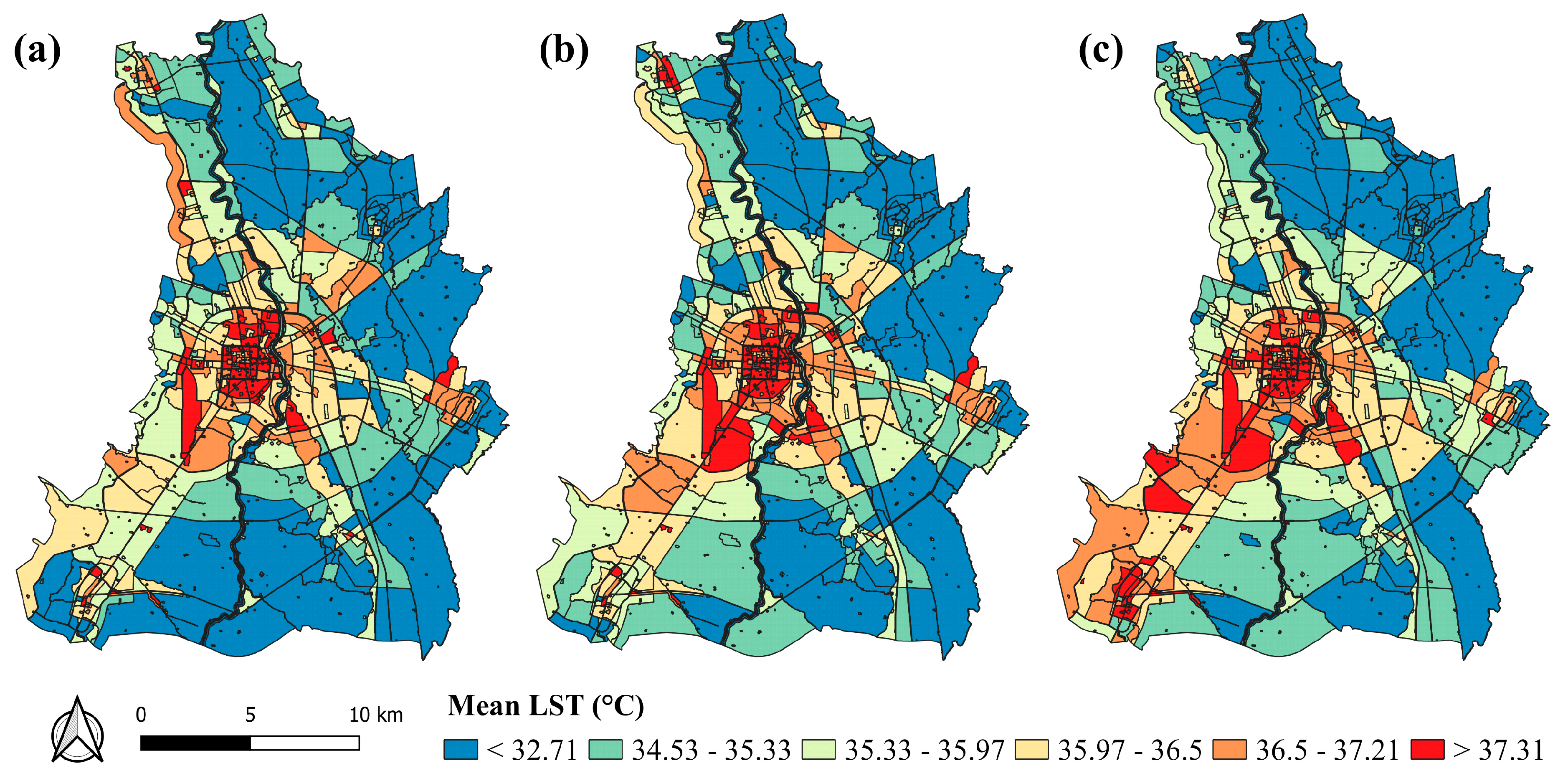
In the final step, the temperature in Kelvin was converted to degrees Celsius by subtracting 273.15. The GIS polygon vector layer of twelve types of LUZs was taken as the basic spatial statistical units, overlaying the three LST years to generate zonal maps displaying the mean LSTs within each LUZ block. The resulting LST is shown in Figure 2.
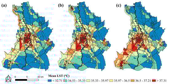
Figure 2.
Spatial distribution maps of mean LSTs in 2017 (a), 2019 (b), and 2023 (c) over the summer.
2.4. Impact of LUZ Categories on LST
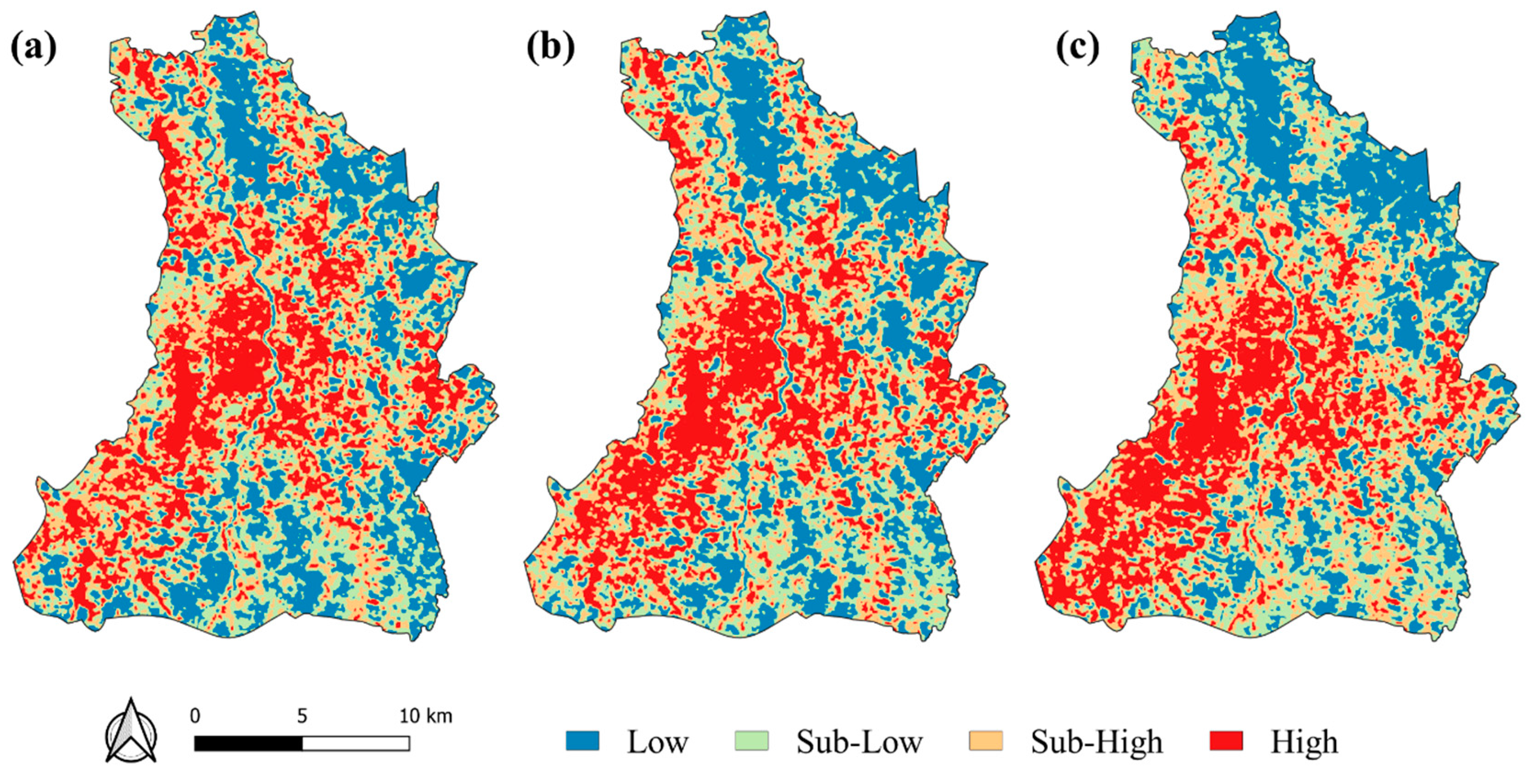
In this study, the distribution index () was used to assess the impact of LUZ on LST through LST distribution patterns in different block categories [20,46]. The “high-temperature center (HTC)” was identified as the highest temperature level using the Jenks natural break classification method [47] (see Figure 3). The calculation formula for can be represented as in (5):
where is the total HTC area, represents the total study area for the LUZ block, and and are the total HTC area and the total area for all LUZ block categories, respectively. A value greater than one indicates that the size of the HTC area in a LUZ block category is larger than that in the entire study area. This suggests that this LUZ block category is the heat source that affects the thermal environment [18]. The spatial distribution of the classified classes is shown in Figure 4.

Figure 3.
Spatial distribution maps of classified LSTs in 2017 (a), 2019 (b), and 2023 (c) over the summer.
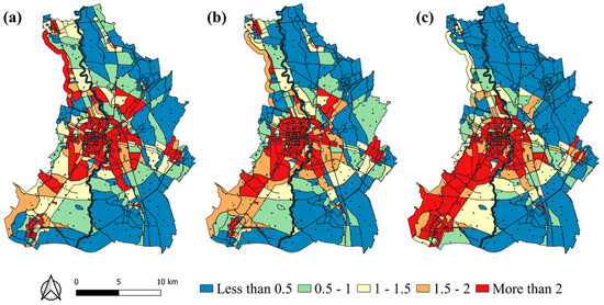
Figure 4.
Land use zoning-based DI maps of the proportion of HTC area in 2017 (a), 2019 (b), and 2023 (c) over the summer.
2.5. Extraction of Surface Biophysical Parameters
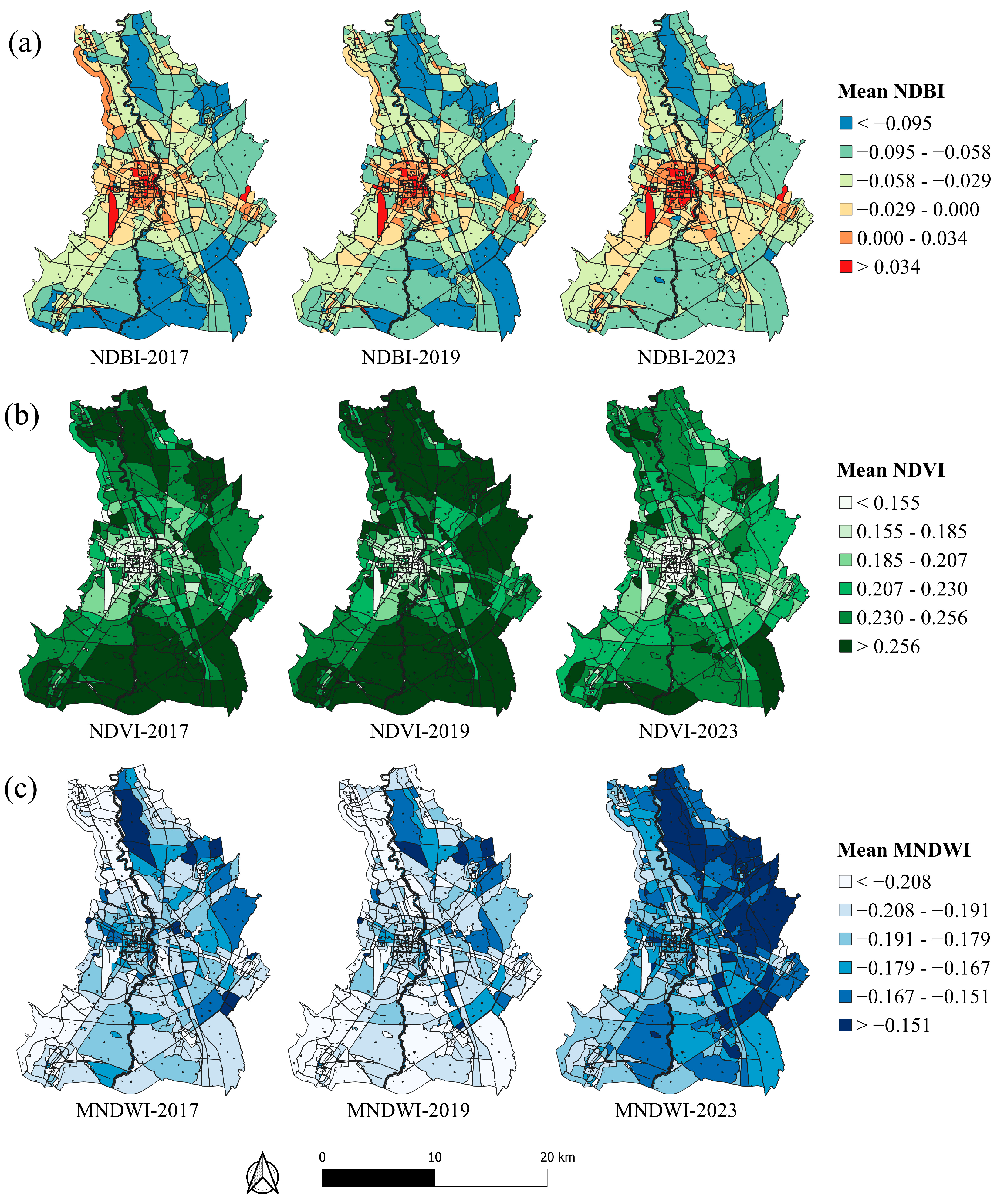
Previous studies have identified certain surface biophysical parameters (SBPs) that affect daily land surface temperature (LST). Studies by Hu et al. [17] and Tian et al. [48] confirmed that the normalized difference vegetation index (NDVI), normalized difference built-up index (NDBI), and modified normalized difference water body index (MNDWI) are suitable for analyzing the factors that drive LST. All the factors were determined at the LUZ block scale by calculating average values, as shown in Table 3 and Figure 5. Therefore, we aimed to analyze the impact of SBPs (NDBI, NDVI, and MNDWI) on LST by characterizing their geographical distribution across LUZ blocks in three periods. Zonal analyses were used to determine the mean LST and SBPs in different LUZ blocks. Figure 6 shows the spatial distribution of SBPs across LUZ blocks. To easily compare the changing situation, the map legend data are divided into strata values that remain the same for each year. The blocks with high NDBI values are primarily located in the central urban areas, while some parts of the surrounding sub-center align with the urban system designed to provide service centers to suburban communities. Meanwhile, blocks with high NDVI and MNDWI values were mostly found in suburban areas with horticultural farming and rice fields.
Table 3.
Description and calculation of driving factors of SUHI.
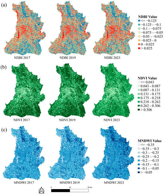
Figure 5.
The surface biophysical parameters of (a) NDBI, (b) NDVI, and (c) MNDWI were derived from Landsat 8 images in 2017, 2019 and 2023.

Figure 6.
Geographical distribution of SBPs (a) NDBI, (b) NDVI, and (c) MNDWI across LUZ blocks in 2017, 2019, and 2023.
2.6. Identifying the Factors That Influence Driving LST
In this study, Pearson’s correlation analysis was used to assess the correlation between the three SBPs for each LUZ category. Afterward, the driving factors that showed a significant correlation with average LST were identified as the correlation factors associated with surface urban heat [33,49]. Moreover, our study utilized a regression analysis to determine the main factors driving LST changes using surface biophysical parameters as independent variables. The best-fit model was identified through stepwise regression analysis (SRA) to account for potential collinearity between variables. This analysis allowed for our understanding of how driving factors of LST vary from past to present due to yearly fluctuations in heat absorption and dissipation by LUZ blocks.
3. Results
3.1. Changes in LST Retrieval across Different LUZs
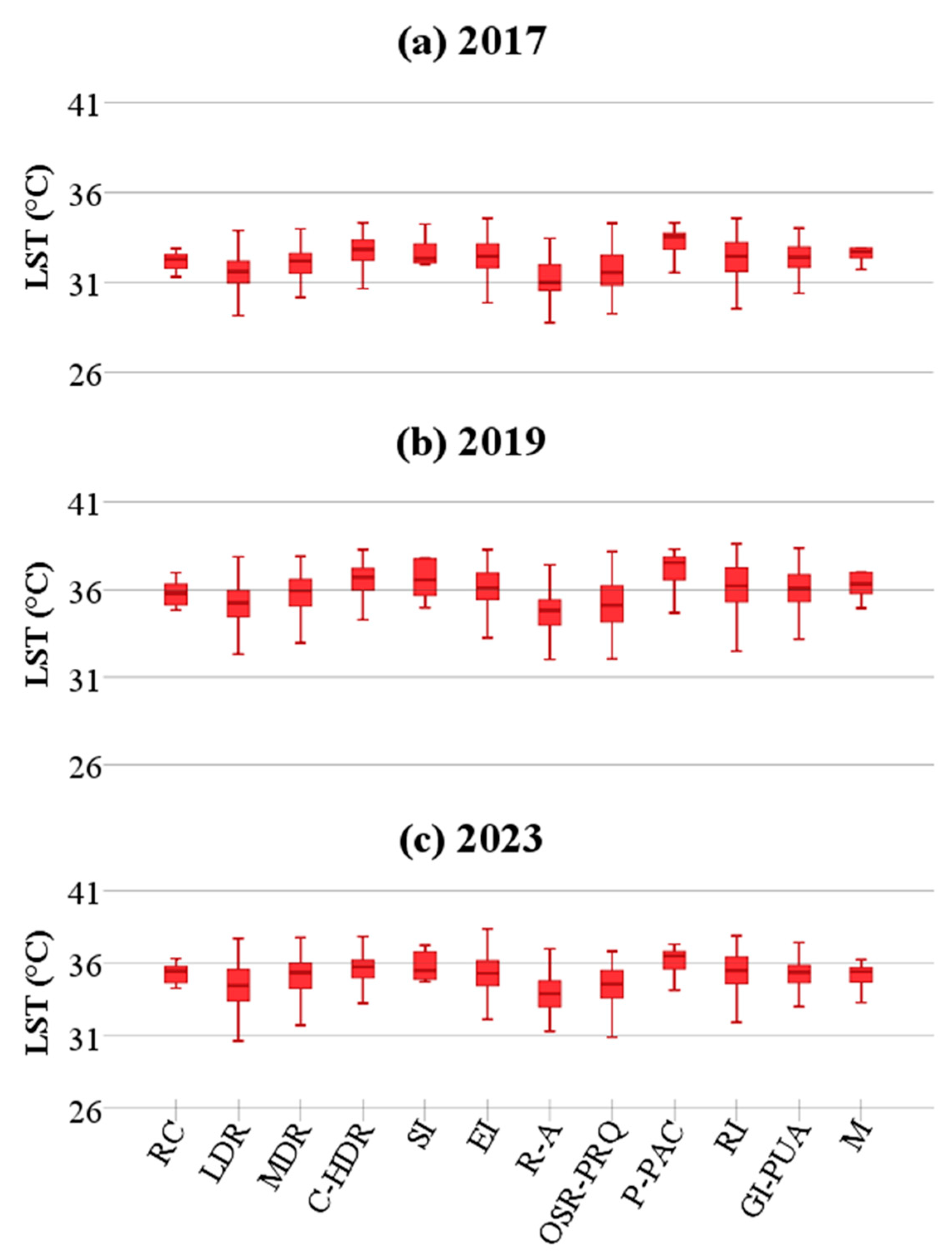
Figure 7 displays the boxplots of the categories of summer LST variations among the twelve types of LUZs. Across the three years, the highest mean LSTs were mainly concentrated in the preserving and promoting arts and culture (P-PAC) zones. The study found that not only the P-PAC but also the specific industrial (SI) zones and military (M) zones had high LSTs. These indicate that there are potential heat sources inside these types of blocks leading to a more significant temperature rise. In contrast, the rural and agricultural (R-A) zones had the lowest average LST for all three years. Throughout the three summers, it can be observed that there were consistent spatial patterns in the distribution of high LST blocks (as depicted in Figure 2). These blocks were primarily located in the main commercial city center of Chiang Mai, extending into the southern Hang Dong district and the southwestern areas between the third ring road and the Hang Dong town center. Based on the analysis, it was found that areas with high urbanization rates and low coverage of green-blue spaces had low greenery and water content. As a result, these areas showed higher temperatures, mainly in residential and development zones of the peri-urban areas, as depicted in Figure 6.
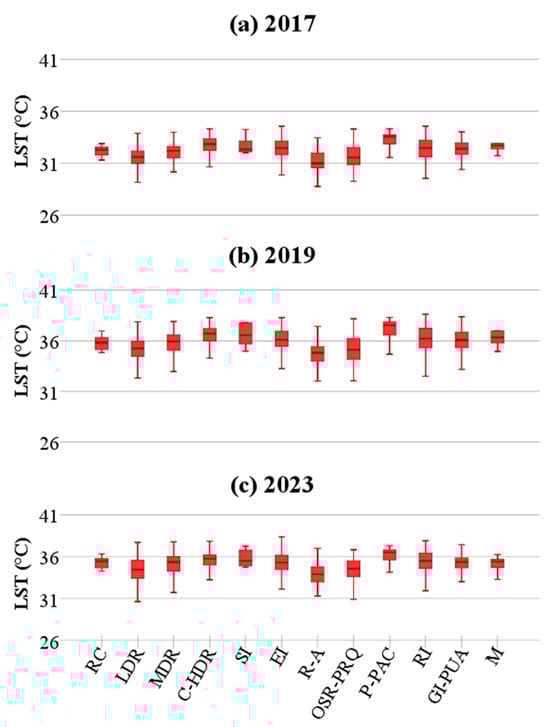
Figure 7.
Boxplots display surface urban heat island variations in different land use zones for summers in (a) 2017, (b) 2019, and (c) 2023.
As part of it, the high-temperature areas are mainly distributed in major business and high-density districts, such as Tha Phae, Chang Klan, Chang Phueak Gate, and Wualai. These areas are developed historic urban districts in the P-PAC mainly composed of residential and commercial areas covered by a highly concentrated built-up index with low greenery and water content. In addition, the industrial and airport-related zones (e.g., SI) located in the south of Chiang Mai International Airport, Airport City, and the military airfield of the Royal Thai Air Force in the military zone were also aggregated hot spots due to high concentrations of heat-absorbing pavement, buildings, airport runways, and other surfaces. In certain parts of the urban fringe areas, such as the Mae Rim and San Sai districts, the temperature was relatively low. These areas have irrigated agricultural lands and nearby wetlands, which create cooling patches within the LUZ blocks and significantly reduce the average surface temperature of these LUZs during summer. The open space for recreation and preserving environmental quality (OSR-PEQ) zones, located near the Mae Ping River, old city moat, canals, and urban parks, also had lower LSTs. This demonstrates the significant cooling effects of large urban ecological parks and water bodies.
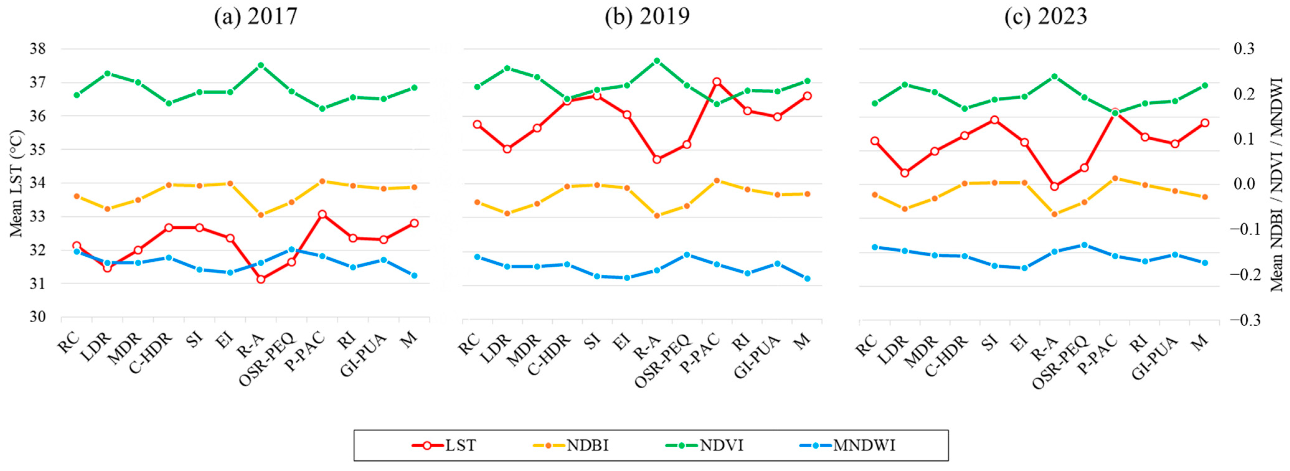
Table 4 shows the mean LST changes among the twelve types of LUZs across the entire Chiang Mai Comprehensive Plan from 2017 to 2023. The annual rate of LST change from 2019 to 2023 showed an overall decrease of 0.19 °C compared to the period from 2017 to 2019, during which there was an increase of 1.85 °C. Between 2019 to 2023, the commercial and high-density residential (C-HDR) zone in the central city of Chiang Mai experienced a 0.25 °C decline in the annual LST rate change. The same average annual decline in LST between 2019 to 2023 was also observed in other types of LUZs but at different rates. LUZs designated for medium to low-density residential and government/public service areas (e.g., P-PAC, EI, RI, GI-PUA, M) showed potential cooling sources from green areas and water within these blocks, resulting in a more significant temperature decrease. The data presented in Figure 8 show that the mean LST variation was influenced by the mean values of the NDBI, NDVI, and MNDWI in each LUZ. It is evident that the P-PAC zone had the highest average LST and NDBI and the lowest average NDVI and MNDWI for all three years. This suggests that these three indices may contribute to the increase in LST. However, it is necessary to determine whether this relationship is statistically significant for all LUZs in order to draw a definitive conclusion.
Table 4.
Mean LST changes in different land use zoning of the entire Chiang Mai Comprehensive Plan from 2017 to 2023.
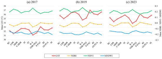
Figure 8.
Dynamics of all three surface biophysical parameters (NDBI, NDVI, MNDWI) and mean LSTs for (a) 2017, (b) 2019, and (c) 2023.
3.2. Spatiotemporal Distribution Characteristics and Changes in LST
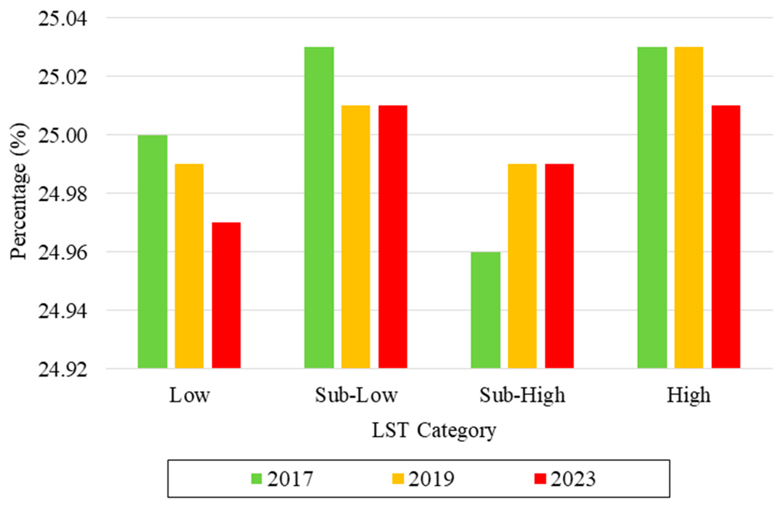
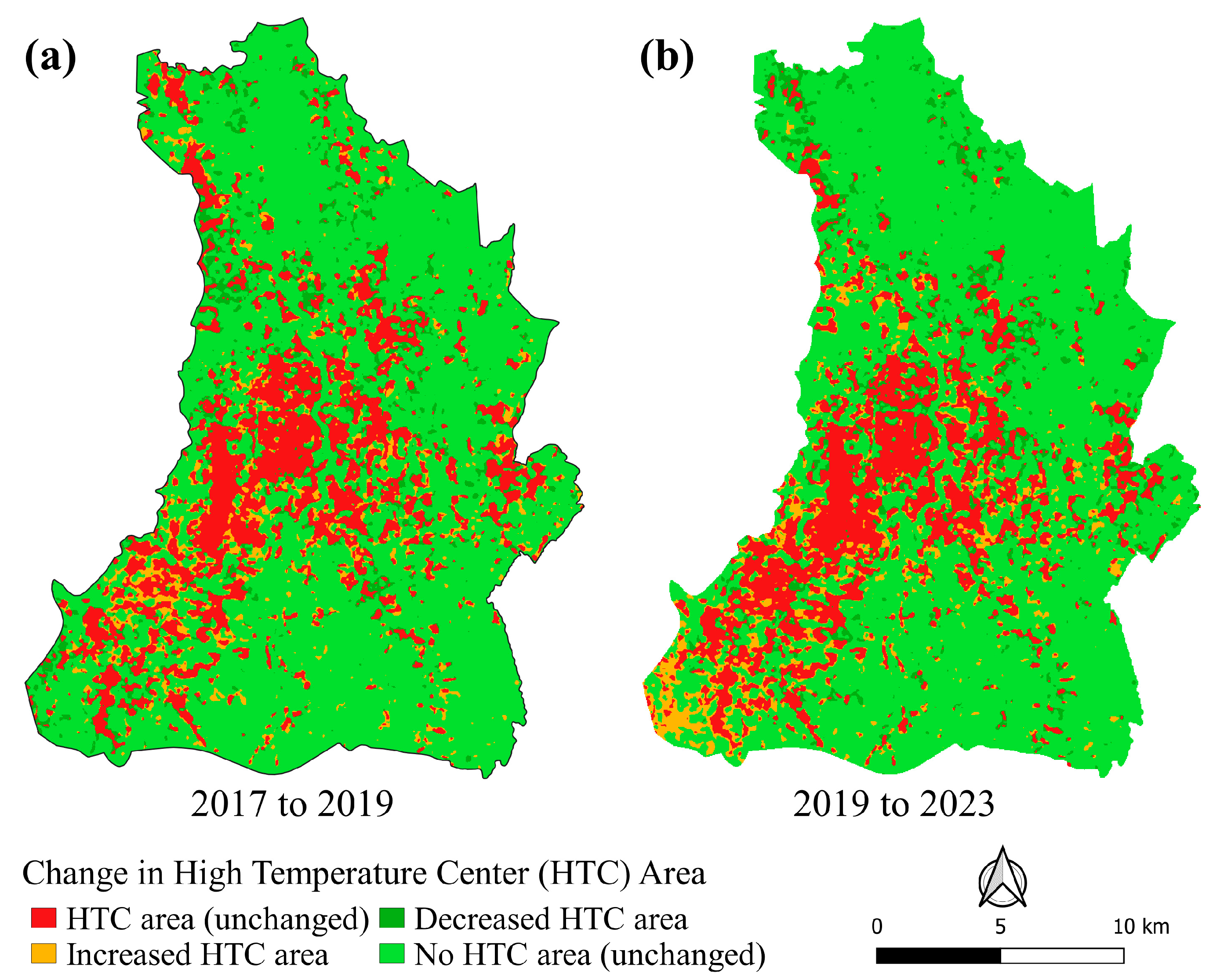
Figure 9 displays the percentage of summer LST categories from 2017 to 2023, which is valuable in studying temperature dynamics over different periods and understanding how they change with varying LST categories. It is evident that the low-LST category continued to decrease from 2017 to 2023, while the high and sub-low categories accounted for more than 25% in all three years. Moreover, the sub-high category saw the most significant increase between 2017 and 2019 and is expected to remain stable between 2019 and 2023. High-level LSTs were mainly distributed from the central city to its outskirts, particularly in Hang Dong, the southern district of the city. This area, which is designated as a low-density residential (LDR) zone, showed an increasing trend in HTC areas for both periods (Figure 10). This indicates that urbanization within these LUZ blocks resulted in potential heat sources, leading to a more significant rise in temperature.

Figure 9.
The proportion for each summer LST category from 2017 to 2023 in the Chiang Mai Comprehensive Plan boundary.

Figure 10.
Change in high-temperature center (HTC) area from (a) 2017 to 2019 and (b) 2019 to 2023.
The classified LST levels change matrix from 2017 to 2019 and 2019 to 2023 revealed the transfer relationship between each LST category (Table 5). It can be observed that the area classified as “no high-temperature center (no HTC)” mainly consisted of cultivated and vacant land, forming the primary composition of the rural and agricultural (R-A) zones within the Comprehensive Plan boundary of Chiang Mai from 2017 to 2023. The agriculture zones mainly consisted of rice fields and horticulture, particularly longan plantations, with off-season farming in irrigated areas. This accounted for approximately 75% (about 307 km2) of the total area in the study region, representing the predominant type among the classified LST levels in the area. It demonstrates that within the urban climate context of Chiang Mai, the agricultural production zone remains a crucial cooling surface, effectively reducing surface temperatures in the Chiang Mai Comprehensive Plan area.
Table 5.
The change matrix of classified LST levels (in km2) from 2017 to 2019 and 2019 to 2023.
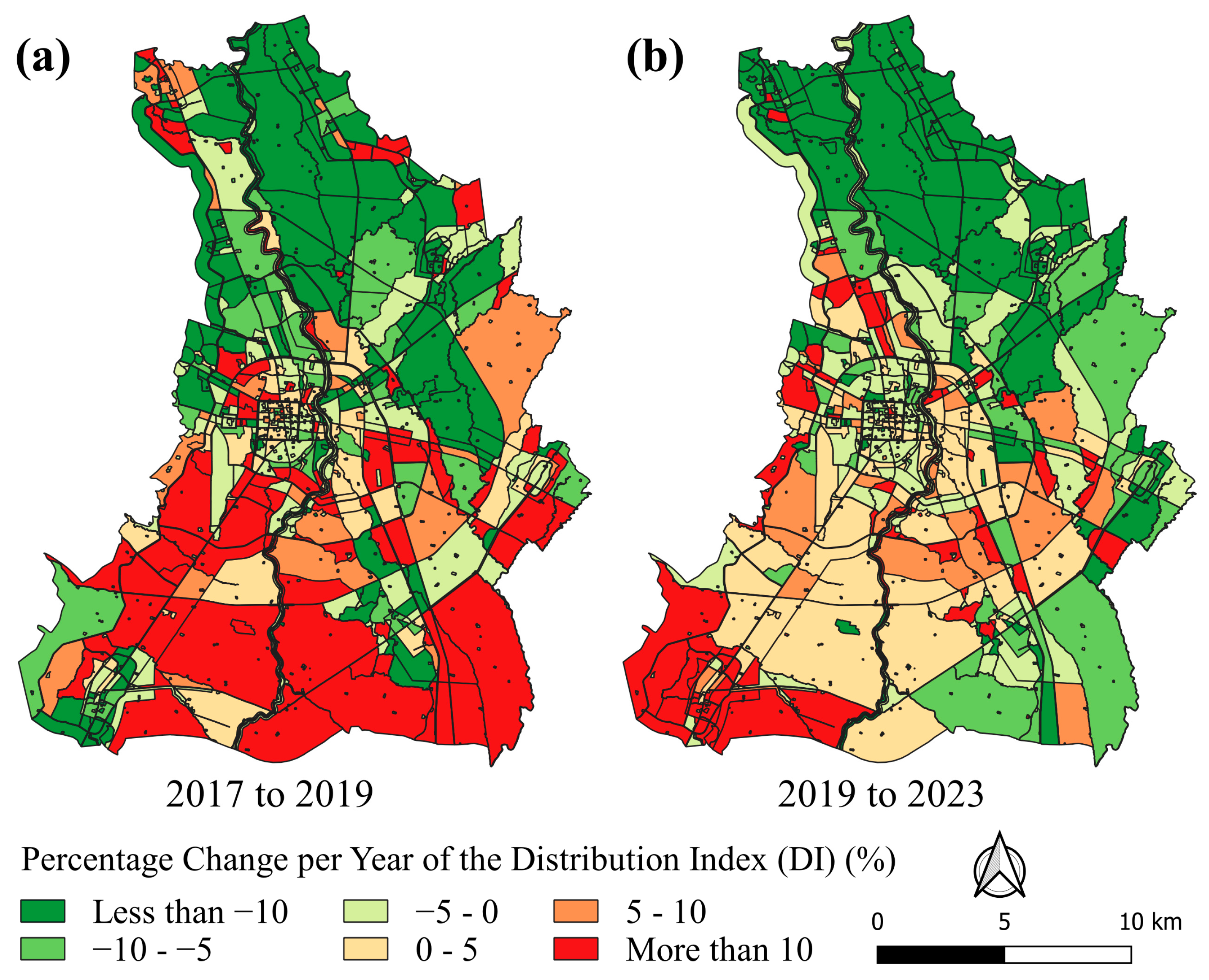
In the past four years (from 2019 to 2023), the HTC area has increased with an annual change rate of 0.02 km2. This continuous expansion of construction land significantly accelerated the urbanization process in Chiang Mai City. This expansion is consistent with the findings of McGrath et al. [41] and Sangawongse [50], who observed that Chiang Mai’s urban area is prone to “urban sprawl”, where settlements expand at low densities, particularly in the southern and eastern sides of the city. Conversely, the expansion of built-up areas in the no HTC area resulted in the replacement of agricultural land with urban land, particularly in the outer ring road areas, where orchard cultivation and rice farming were once prevalent [51]. Similarly, the highest increase in the percentage annual rate of change in the DI value (0.060) occurred in the RC zone from 2019 to 2023 (Table 6). This suggests that the RC zone had the most significant contribution to the SUHI effect among the inner-city historic districts. This was followed by zones LDR, MDR, SI, and RI (0.021, 0.016, 0.009, 0.008, respectively); as Chiang Mai’s urban fringe expands, the proportion of the HTC area is also increasing (see Figure 11).
Table 6.
Average percentage annual rates of change in the DI and percentage of DI types in the total study area from 2007 to 2019 and 2019 to 2023.

Figure 11.
Spatial distributions of the percentage annual rates of change in the DI from (a) 2017 to 2019 and (b) 2019 to 2023.
However, the impact of the DI values on LST was not prominent in the C-HDR zones. On the other hand, the C-HDR zones produced lower DI values than other development promotion areas, and the C-HDR block witnessed a low DI value (DI value less than 0), decreasing by −0.031 from 2017 to 2019. The lowest DI value was recorded at −0.085 from 2019 to 2023 in the summer. This indicates that increasing cool sources correspond to cooling effects in the commercial and high-density residential zones. This could be due to landowners transforming their vacant land into agricultural land in the C-HDR zone to avoid taxes. They do this to benefit from a lower land tax rate than the one applied to vacant land before the new Land and Building Tax Act, B.E. 2562 (2019), was put into effect on 13 March 2019 [52]. These results suggest that spatiotemporal thermal variations within LUZs may be influenced by surface biophysical parameters in these zones. These results clarify that the HTC area significantly impacted the SUHI effect in five significant LUZs located in the central to southern part of the Chiang Mai Comprehensive Plan (Figure 12).
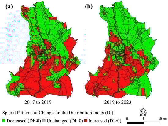
Figure 12.
Spatial patterns of changes in the DI from 2017–2019 (a) and 2019–2023 (b).
3.3. Relative Importance of SBPs’ Effects on LST in Different LUZs
The scatter plot in Figure 13a indicates that NDBI, which represents the spectral indicator of the impervious surface layer, was positively and linearly associated with the LSTs of three periods, namely 2017, 2019, and 2023, with correlation coefficient values of 0.452, 0.524, and 0.447, respectively. Changes in the development of urban construction can lead to variations in underlying surface properties, which can significantly impact the SUHI in different LUZs. However, vegetation and water can have a positive effect in mitigating the SUHI impact. Figure 13b,c demonstrates a negative linear correlation between NDVI and MNDWI, which represent vegetation coverage and water content, respectively, with LSTs in hot seasons, leading to a reduction in Chiang Mai City’s UHI. However, a weak linear relationship between them was observed in summer LSTs, especially in MNDWI. According to our results, the change in correlation coefficients of MNDWI with LSTs ranged from 0.033 to approximately 0.199 from 2017 to 2023. This value is relatively low compared to other SBPs. Even with the low correlation coefficient values, this factor still plays a driving factor in the city’s heat warming.
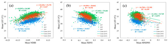
Figure 13.
Scatter plots depicting the relationship between mean LSTs and SBPs for (a) NDBI, (b) NDVI, and (c) MNDWI.
The influence of three potential SBPs as driving factors on summer LSTs in different LUZs was assessed using Pearson correlation coefficients. Furthermore, to elucidate the influence of SBPs on land use control ordinances among LUZs, a three-period summer LST driving analysis is presented in Table 7. It was found that certain SBPs have a significant impact on the thermal environment and contribute to LSTs. These parameters include characteristics of impervious urban surfaces, vegetation-covered lands, and water content surfaces, and consistently contribute to higher summer LSTs on the LUZ block scale. NDBI was significantly correlated (p < 0.01) with summer LSTs for the built-up parameter, signifying that surfaces covered by built-up areas often exhibited high LSTs. Additionally, the correlation results for NDBI and LST showed a positive relationship in all periods ( = 0.672, = 0.724, and = 0.668), implying that this surface biophysical parameter may contribute to an increasing tendency in the summer SUHI effect. Furthermore, the impact of NDBI on summer LST (e.g., 2023 = 0.668) was more significant than that of NDVI and MNDWI (e.g., 2023 = −0.580 and 2023 = −0.446, respectively). The analyzed data indicate that areas with water and vegetation, as shown by NDVI and MNDWI, had a significant negative correlation (p < 0.01) with LST during all periods. This suggests that urban areas with plenty of green and blue spaces have the potential to reduce heat within LUZ blocks across all studied periods. In some periods, the relationship between SBPs and LST in certain LUZs became nonsignificant (p > 0.05), e.g., RC, SI, EI, P-PAC, RI, GI-PUA, and M. These results illustrate that SBPs have a significant influence on LST in certain LUZs. The variations can be influenced by development in the LUZ block. When built-up areas expand, there is less vegetation and water cover, which reduces their ability to moderate high temperatures and may increase LST levels in most LUZ block types. However, our study results indicate that the observed decrease in average LST in Chiang Mai from 2019 to 2023 may be influenced by various factors beyond built-up expansion. While urbanization and changes in land cover are important factors affecting LST, other elements like changes in weather patterns, atmospheric conditions, and land use management practices can also play significant roles.
Table 7.
Results of correlation analyses between SBPs and summer LSTs.
To determine the main driving factors on LST for different LUZ block categories, the stepwise regression analysis (SRA) was used to select the best-fit model from all possible subset models. The three driving factors of the SBPs were selected, and models for the twelve LUZ block categories were created separately. At a 95% confidence level, all coefficients in the best subsets regression model were significant because their p-values were less than 0.05. Considering all periods, SBPs could explain 45.7–53.2% of the summer LST variations in the three years. Meanwhile, the LUZ block categories considered in this study explained 12.8–85.4%, 24.5–75.3%, and 28.3–81.9% of the SUHI variations for the twelve separate models in 2017, 2019, and 2023, respectively, except RC, which could not explain the LST variations. Yearly variations in summer LST were observed across different LUZ block types in 2019. NDBI and NDVI were found to be the primary drivers of LST for all categories, while MNDWI did not exhibit any influence on LST.
Table 8 ranks the driving effects of three SBPs on LUZ block categories across three observation years. Between 2017 and 2023, the standardization coefficient for summer LST fluctuated from 13.948 to 16.041 (2017 to 2019) and decreased to 15.047 in 2023 for all LUZ block categories based on the stepwise regression analysis. There was a significant impact of NDBI on LST for most types of blocks, while NDVI and MNDWI had a noticeable impact on LST for most LUZ block types, especially during the summer of 2023. This could be because of the impact of the Land and Building Tax Act B.E. 2562 (2019), which affects the conversion of vacant lands into agricultural lands to gain tax advantages, loopholes, and avoidance [52,53]. Additionally, off-season rice farming took place in irrigated areas on the northeastern side of the suburban area during the dry season from November to April to meet the increased demand for rice exports in 2023 [54]. However, it was the main influencing factor for all block types except for seven LUZ categories (RC, MDR, C-HDR, SI, R-A, OSR-PEQ, and M). It had a changing negative driving effect on LST in different years, such as 2017 and 2019. For MNDWI, the negative driving effect on LST became very weak and was noted for some LUZ block types in 2017 (i.e., LDR, MDR) and 2023 (i.e., R-A, RI, GI-PUA); however, this driving effect was nonsignificant during the summer of 2019 for all block types. In Chiang Mai, different types of neighborhoods experience varying factors that contribute to the increase in LST during the summer season. The NDBI had a positive effect on LST, while the NDVI and MNDWI had the opposite effect. This pattern indicates that the urban landscape’s impervious surfaces, vegetation cover, and water bodies have the most significant effect on SUHI. The study highlights that NDBI is the main cause of SUHI, while NDVI is the second most significant factor. The combined effect of NDVI and NDBI exhibits the high explanatory power concerning SUHI in the Chiang Mai Comprehensive Plan area.
Table 8.
Best subsets regression between SBPs and LST for various LUZ block categories across three observation years.
4. Discussion
4.1. Summer Variations in Driving Factors on LST
This study found that the SBPs, such as NDBI and NDVI, were better predictors of summer LST patterns in Chiang Mai City than MNDWI. Therefore, these spectral indices are suitable for reflecting surface information and can be used for LST prediction or downscaling, especially in urban areas. Our findings were consistent with previous studies that have also shown the effectiveness of these indices [5,48,55]. According to this study, it is suggested that local government organizations who approve land use should adopt stringent measures to control impervious surfaces while supporting the growth of green spaces. This is necessary because the spatial arrangement of summer land surface temperature and the factors influencing it must be considered when devising heat mitigation strategies for the area under their jurisdiction.
In the urban fringe areas, rural and agricultural zones with high-water content surfaces can help reduce the impact of increased temperatures during the hot season. Therefore, it is essential to implement measures to control changes in land use in agricultural areas and wetlands. Increasing urban greenery coverage during lush vegetation growth can also help cool surfaces in LUZs by providing shading and interacting with radiation. On the other hand, industrial and airport-related zones have a high concentration of heat-absorbing pavements, buildings, and other surfaces, which generate extremely high LST. To mitigate these effects, design interventions such as cool pavements and incorporating blue-green spaces in their surroundings can be implemented. These measures can also help alleviate the negative impact of anthropogenic heat emissions on the surrounding LUZ blocks to a certain extent.
4.2. Effects of Land Use Zoning Block Categories on Summer LSTs
The main contributions of this study are twofold: firstly, it characterizes and distributes the zoning regulations of land use for block-scale LST spatial patterns, and secondly, it interprets the effects of surface biophysical multifactorial driving on surface heat island changes from the urban land use planning perspective. In the central part of Chiang Mai City, high-temperature areas with elevated surface temperature levels were found to be concentrated in commercial-residential and industrial zones. The lack of vegetation coverage in highly developed blocks reduces evaporative cooling and shading effects, resulting in elevated LST levels [56]. It is important to consider that the consequences of land use planning can vary depending on the type of surface and other functional controls. To gain a better understanding of the laws governing the formation of urban heat islands, it may be necessary for future studies to use multi-temporal techniques such as seasonal variation, nocturnal effects, and multi-regional experiments. Such experiments could help to identify more general factors that contribute to the formation of UHIs.
Our research has shown that the impact of various types of urban blocks on the summer surface thermal environment varies depending on the observation period. Additionally, the thermal contrasts between block types exhibit different patterns throughout the warmest months. For example, our stepwise regression model has revealed that each urban block has its own set of driving factors that influence summer LSTs. Blocks that have a higher concentration of built-up areas typically exhibit higher LSTs. The most significant factor that contributes to a decrease in LSTs is NDVI, particularly during summer. Therefore, in these areas, uncovered land and surfaces impervious to water (quantified by NDBI) have a more significant influence on summer LSTs’ rise than NDVI. These findings are consistent with earlier studies that identified building density or vegetation coverage as the primary drivers of surface temperature variations [57,58,59]. Our research has enhanced our knowledge of how urban land use planning impacts and changes summer heat island variations in a tropical city in Thailand.
4.3. Implications for Land Use Planning on Urban Climate Changes
The ineffective implementation of land use regulation and uncontrolled urban development has led to significant urban thermal environment challenges and worsened the heat island effect in numerous Asian cities. This has led to residents experiencing high-temperature stress, which is unprecedented [60]. Even though previous research has measured the connection between spectral indices and SUHI in Chiang Mai, the spatial variation in LST and its relationship with land use/land cover, temperature differences across different land use zones [61,62,63,64], and multidimensional indicators in quantitative research on biophysical parameters and LSTs have often been overlooked. By conducting a detailed analysis at the local scale, we aimed to provide valuable insights into the spatial differences in temperature patterns and the factors contributing to the heat island effect in Chiang Mai. Integrating these variables into our analysis gave us a more comprehensive understanding of the factors that influence temperature variations in urban environments. Our research confirmed that the land surface temperature in urbanized areas varies over the hot seasons within the urban land use plan of Chiang Mai City. During the summer daytime, regions with high temperatures were mainly in areas of medium to low-rise residential zones. At the same time, they were scattered around industrial zones near major transportation hubs, such as airports. This phenomenon of spatial patterns can be explained by the fact that impervious surfaces covered by built-up areas can absorb and retain more solar radiation during the summer than other surface covers, such as urban green spaces or vegetation land [65]. In contrast, surface water bodies possess a high specific heat capacity surface, which results in their slower warming-up speed. This makes water bodies function as exceptional islands during the daytime, as noted by Oke [66], Zhao et al. [67], Gunawardena et al. [68], and Yao et al. [20]. Specifically, cultivated areas with water, such as paddy fields, can have a cooling effect in the urban fringe areas.
Our analysis revealed that dense vegetation by NDVI had the most significant impact on LST during summer daytime in specific block types, such as rural and agricultural zones, religious institution zones, government institutes, public utilities, and amenities zones. These areas have significant vegetation cooling potential, which attempts to reduce urban heat islands and indirectly increase the comfort of living in outdoor environments. This finding is supported by studies conducted by Sabrin et al. [69], Lai et al. [70], and Sarfo et al. [71]. This underscores the need for planning and conserving green spaces for sustainability in these areas. Given this fact, it is undoubtedly an opportunity for the entire urban area to contemplate mitigation strategies concerning vegetation during urban planning and local/microscale urban design. Expanding green areas would be beneficial, but strategic vegetation placement can further enhance the advantages and local thermal comfort in open spaces while decreasing the cooling energy demand for buildings [72,73].
4.4. Limitations and Prospective Research
Our research aimed to study the SUHI effect by analyzing thermal remote sensing. However, we did not explore the relationship between the remotely sensed land surface temperature and surface air temperature (SAT) in our study, which has been previously examined by Coseo and Larsen [74] and Ivajnsic et al. [75]. SAT refers to the temperature at pedestrian height within the urban canopy and plays a significant role in shaping urban thermal environments and human thermal comfort [76]. Therefore, future studies should consider the interplay between LST and SAT. However, LST provides extensive coverage and high spatial resolution data with temporal resolution, making it advantageous for research. Moreover, our research focused on studying the SUHI effect using thermal remote sensing. Due to limitations, we could not employ a comprehensive accuracy evaluation methodology. Climate data preceding Landsat-8 image acquisition (2017, 2019, and 2023) from the Chiang Mai Station of the Thai Meteorological Department informed weather conditions. Future research should rigorously assess accuracy by comparing satellite-derived LST with ground-based measurements and existing LST products. Pearson correlation analysis and stepwise regression are two commonly used statistical methods due to their simplicity and effectiveness. However, these methods rely on linear and normal distribution assumptions, and their results can be affected by collinearity between independent variables [17]. Moreover, the use of earlier models, such as stepwise regression, may make it difficult to determine the relative importance of all factors. Therefore, to address these limitations, further studies are needed to employ machine learning models such as random forest (RF), support vector regression (SVR), artificial neural network (ANN), etc. These models do not rely on linear and normal distribution assumptions and are robust against the multivariate collinearity of independent variables. They can further rank the explanatory rates of multiple factors [77,78,79]. Further research is needed to investigate the relationship, connection, and causation between surface temperature time series and various urban regions. These complex systems often have nonlinear and non-separable dynamic interactions, which makes traditional approaches to causal inference, such as statistical correlation, impractical or ineffective [80].
Acquiring comprehensive three-dimensional (3D) building GIS data on a large scale in our study area in Thailand was challenging despite the fact that building structures are crucial components of urban morphologies and critical contributors to the UHI. Therefore, our research focused on investigating the impact of surface biophysical parameters, which are two-dimensional (2D) land surface properties quantified by NDBI, NDVI, and MNDWI. These parameters reflect the underlying surface’s physical properties, as Tian et al. [48] described. There are still several areas of research that require further investigation and attention in future studies regarding the factors that drive surface temperature. For instance, a study should investigate the role of building morphological parameters derived from 3D building databases—building height, building coverage ratio (BCR), sky view factor (SVF), floor area ratio (FAR), frontal area index (FAI), etc.—to understand the diurnal variations in LST. Some studies, such as Scarano and Mancini [81], Sun et al. [82], Ma et al. [83], and Hu et al. [17], have already explored this area and can provide valuable insights.
5. Conclusions
This study examines the driving factors behind summer land surface temperature patterns in urban land use zones over three years. Ultimately, we observed that LUZs with higher built-up surfaces and less greenery tend to experience higher LST during the hot season in Chiang Mai. As the proportion of impermeable surfaces, such as pavement and buildings, increases within urban land use zones, the LSTs during Chiang Mai’s hot seasons also increase. The contribution of high-density development areas to high-temperature extreme regions is significant in medium-low-rise development, industrial, and historical conservation areas (LDR, MDR, RC, and SI). This is due to modern mid-rise buildings, low-density peri-urban housing projects, and industrial development. On the other hand, high-rise areas (C-HDR) with cool surfaces, such as vegetation and water bodies, exhibited low distribution index values, indicating a fragile negative driving effect on surface temperature during hot summers. Therefore, it is important to note that building shadows can significantly impact summer LST in high-density zones [17,84,85]. The results of the stepwise multiple regression analysis indicate that the impact of remotely sensed surface temperature on the urban environment is impacted by the different zoning functions of the Chiang Mai Land Use Plan. This study found that built landscape elements that were mainly impervious surfaces had a more significant contribution to surface temperature variations under high temperatures. At the same time, the cooling variables that indicated green spaces generally determined more variations during summer seasons. To promote sustainable urban cooling, it is necessary to implement zoning regulations prioritizing green spaces and incentive schemes to protect and encourage them. Additionally, limiting the use of heat-absorbing materials can help reduce the intensity of LST. These strategies can help cities take action toward sustainable urban cooling.
Author Contributions
Conceptualization, Damrongsak Rinchumphu and Manat Srivanit; methodology, Damrongsak Rinchumphu and Manat Srivanit; software, Manat Srivanit and Niti Iamchuen; formal analysis, Manat Srivanit; resources, Damrongsak Rinchumphu and Manat Srivanit; writing—original draft preparation, Manat Srivanit; writing—review & editing, Damrongsak Rinchumphu, Manat Srivanit, Niti Iamchuen, and Chuchoke Aryupong; visualization, Manat Srivanit; supervision, Damrongsak Rinchumphu and Chuchoke Aryupong; project administration, Damrongsak Rin-chumphu and Manat Srivanit; funding acquisition, Damrongsak Rinchumphu. All authors have read and agreed to the published version of the manuscript.
Funding
This research project was supported by Fundamental Fund 2023, Chiang Mai University. The grant number is R65EX00154 under the project “Sustainable Climate-Urban-Water Resilience and Food Cycle Community Chiang Mai City Management”.
Data Availability Statement
The dataset is available on request from the authors.
Acknowledgments
We would like to express our gratitude to the support staff at City Research and Development Center (City R&D), Faculty of Engineering, Chiang Mai University for their assistance. Furthermore, we extend our heartfelt thanks to the Faculty of Architecture and Planning, Thammasat University, for providing us with the necessary facilities for our collaborative research activities.
Conflicts of Interest
The authors declare no conflicts of interest.
Appendix A. The Climate Conditions and Precipitation on a Daily Basis during the Study Periods
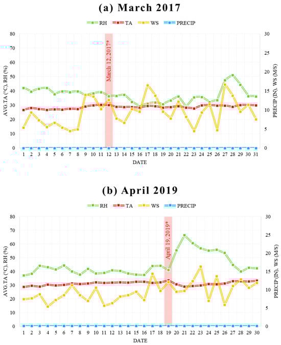
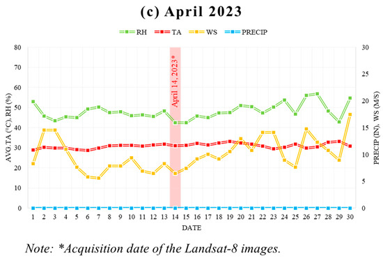
Figure A1.
The Chiang Mai Station of the Thai Meteorological Department shared the average daily climate conditions, including relative humidity (RH), air temperature (TA), and wind speed (WS), as well as precipitation data (PRECIP), for the acquisition of Landsat-8 images in 2017, 2019, and 2023.
Figure A1.
The Chiang Mai Station of the Thai Meteorological Department shared the average daily climate conditions, including relative humidity (RH), air temperature (TA), and wind speed (WS), as well as precipitation data (PRECIP), for the acquisition of Landsat-8 images in 2017, 2019, and 2023.

References
- United Nations, Department of Economic and Social Affairs, Population Division. World Population Prospects 2022: Summary of Results; UN DESA/POP/2021/TR/NO. 3; United Nations: New York, NY, USA, 2022.
- Nguyen, C.T.; Chidthaisong, A.; Limsakul, A.; Varnakovida, P.; Ekkawatpanit, C.; Diem, P.K.; Diep, N.T.H. How do disparate urbanization and climate change imprint on urban thermal variations? A comparison between two dynamic cities in Southeast Asia. Sustain. Cities Soc. 2022, 82, 103882. [Google Scholar] [CrossRef]
- Estoque, R.C.; Murayama, Y.; Myint, S.W. Effects of landscape composition and pattern on land surface temperature: An urban heat island study in the megacities of Southeast Asia. Sci. Total Environ. 2017, 577, 349–359. [Google Scholar] [CrossRef] [PubMed]
- Estoque, R.C.; Murayama, Y. Intensity and spatial pattern of urban land changes in the megacities of Southeast Asia. Land Use Policy 2015, 48, 213–222. [Google Scholar] [CrossRef]
- Wang, Y.; Chen, L.; Kubota, J. The relationship between urbanization, energy use and carbon emissions: Evidence from a panel of Association of Southeast Asian Nations (ASEAN) countries. J. Clean. Prod. 2016, 112, 1368–1374. [Google Scholar] [CrossRef]
- Stewart, I.D.; Oke, T.R. Local climate zones for urban temperature studies. Bull. Am. Meteorol. Soc. 2012, 93, 1879–1900. [Google Scholar] [CrossRef]
- Kalnay, E.; Cai, M. Impact of urbanization and land-use change on climate. Nature 2003, 423, 528–531. [Google Scholar] [CrossRef] [PubMed]
- Varnakovida, P.; Ko, H.Y.K. Urban expansion and urban heat island effects on Bangkok metropolitan area in the context of eastern economic corridor. Urban Clim. 2023, 52, 101712. [Google Scholar] [CrossRef]
- Dararat, K.; Shobhakar, D. Time series analysis of land use and land cover changes related to urban heat island intensity: Case of Bangkok metropolitan area in Thailand. J. Urban Manag. 2020, 9, 383–395. [Google Scholar]
- Mokarram, M.; Taripanah, F.; Pham, T.M. Investigating the effect of surface urban heat island on the trend of temperature changes. Adv. Space Res. 2023, 72, 3150–3169. [Google Scholar] [CrossRef]
- Mohammad Harmay, N.S.; Choi, M. The urban heat island and thermal heat stress correlate with climate dynamics and energy budget variations in multiple urban environments. Sustain. Cities Soc. 2023, 91, 104422. [Google Scholar] [CrossRef]
- Verichev, K.; Salazar-Concha, C.; Díaz-López, C.; Carpio, M. The influence of the urban heat island effect on the energy performance of residential buildings in a city with an oceanic climate during the summer period: Case of Valdivia, Chile. Sustain. Cities Soc. 2023, 97, 104766. [Google Scholar] [CrossRef]
- Ulpiani, G. On the linkage between urban heat island and urban pollution island: Three-decade literature review towards a conceptual framework. Sci. Total Environ. 2021, 751, 141727. [Google Scholar] [CrossRef] [PubMed]
- Wang, Y.; Guo, Z.; Han, J. The relationship between urban heat island and air pollutants and them with influencing factors in the Yangtze River Delta, China. Ecol. Indic. 2021, 129, 107976. [Google Scholar] [CrossRef]
- Fahed, J.; Kinab, E.; Ginestet, S.; Adolphe, L. Impact of urban heat island mitigation measures on microclimate and pedestrian comfort in a dense urban district of Lebanon. Sustain. Cities Soc. 2020, 61, 102375. [Google Scholar] [CrossRef]
- Chen, S.; Bao, Z.; Ou, Y.; Chen, K. The synergistic effects of air pollution and urban heat island on public health: A gender-oriented nationwide study of China. Urban Clim. 2023, 51, 101671. [Google Scholar] [CrossRef]
- Hu, D.; Meng, Q.; Schlink, U.; Hertel, D.; Liu, W.; Zhao, M.; Guo, F. How do urban morphological blocks shape spatial patterns of land surface temperature over different seasons? A multifactorial driving analysis of Beijing, China. Int. J. Appl. Earth Obs. Geoinf. 2022, 106, 102648. [Google Scholar] [CrossRef]
- Huang, X.; Wang, Y. Investigating the effects of 3D urban morphology on the surface urban heat island effect in urban func-tional zones by using high-resolution remote sensing data: A case study of Wuhan, Central China. ISPRS J. Photogramm. Remote Sens. 2019, 152, 119–131. [Google Scholar] [CrossRef]
- Weng, Q. Thermal infrared remote sensing for urban climate and environmental studies: Methods, applications, and trends. ISPRS J. Photogramm. Remote Sens. 2009, 64, 335–344. [Google Scholar] [CrossRef]
- Yao, X.; Zhu, Z.; Zhou, X.; Shen, Y.; Shen, X.; Xu, Z. Investigating the effects of urban morphological factors on seasonal land surface temperature in a “Furnace city” from a block perspective. Sustain. Cities Soc. 2022, 86, 104165. [Google Scholar] [CrossRef]
- Li, X.; Yang, B.; Xu, G.; Liang, F.; Jiang, T.; Dong, Z. Exploring the impact of 2-D/3-D building morphology on the land sur-face temperature: A case study of Three Megacities in China. IEEE J. Sel. Top. Appl. Earth Obs. Remote Sens. 2021, 14, 4933–4945. [Google Scholar] [CrossRef]
- Grigoras, G.; Uritescu, B. Land Use/Land Cover changes dynamics and their effects on Surface Urban Heat Island in Bucharest, Romania. Int. J. Appl. Earth Obs. Geoinf. 2019, 80, 115–126. [Google Scholar] [CrossRef]
- Li, B.; Chen, Y.; Shi, X. Does elevation dependent warming exist in high mountain Asia? Environ. Res. Lett. 2020, 15, 024012. [Google Scholar] [CrossRef]
- Kotharkar, R.; Ramesh, A.; Bagade, A. Urban Heat Island studies in South Asia: A critical review. Urban Clim. 2018, 24, 1011–1026. [Google Scholar] [CrossRef]
- Stewart, I.D. A systematic review and scientific critique of methodology in modern urban heat island literature. Int. J. Climatol. 2011, 31, 200–217. [Google Scholar] [CrossRef]
- Iamtrakul, P.; Padon, A.; Chayphong, S. Quantifying the Impact of Urban Growth on Urban Surface Heat Islands in the Bangkok Metropolitan Region, Thailand. Atmosphere 2024, 15, 100. [Google Scholar] [CrossRef]
- Sanecharoen, W.; Nakhapakorn, K.; Mutchimwong, A.; Jirakajohnkool, S.; Onchang, R. Assessment of Urban Heat Island Patterns in Bangkok Metropolitan Area Using Time-Series of LANDSAT Thermal Infrared Data. Environ. Nat. Resour. J. 2019, 17, 87–102. [Google Scholar] [CrossRef]
- Khamchiangta, D.; Dhakal, S. Future urban expansion and local climate zone changes in relation to land surface temperature: Case of Bangkok Metropolitan Administration, Thailand. Urban Clim. 2021, 37, 100835. [Google Scholar] [CrossRef]
- Adulkongkaew, T.; Satapanajaru, T.; Charoenhirunyingyos, S.; Singhirunnusorn, W. Effect of land cover composition and building configuration on land surface temperature in an urban-sprawl city, case study in Bangkok Metropolitan Area, Thailand. Heliyon 2020, 6, e04485. [Google Scholar] [CrossRef] [PubMed]
- Keeratikasikorn, C.; Bonafoni, S. Urban Heat Island Analysis over the Land Use Zoning Plan of Bangkok by Means of Landsat 8 Imagery. Remote Sens. 2018, 10, 440. [Google Scholar] [CrossRef]
- Du, H.Y.; Song, X.J.; Jiang, H.; Kan, Z.H.; Wang, Z.B.; Cai, Y.L. Research on the cooling island effects of water body: A case study of Shanghai, China. Ecol. Indic. 2016, 67, 31–38. [Google Scholar] [CrossRef]
- Simon, O.; Yamungu, N.; Lyimo, J. Simulating land surface temperature using biophysical variables related to building density and height in Dar Es Salaam, Tanzania. Geocarto Int. 2023, 38, 1–18. [Google Scholar] [CrossRef]
- Yao, X.; Zeng, X.; Zhu, Z.; Lan, Y.; Shen, Y.; Liu, Q.; Yang, F. Exploring the diurnal variations of the driving factors affecting block-based LST in a “Furnace city” using ECOSTRESS thermal imaging. Sustain. Cities Soc. 2023, 98, 104841. [Google Scholar] [CrossRef]
- Yao, X.; Zhu, Z.; Zeng, X.; Huang, S.; Liu, Q.; Yu, K.; Zhou, X.; Chen, Z.; Liu, J. Linking maximum-impact and cumula-tive-impact indices to quantify the cooling effect of waterbodies in a subtropical city: A seasonal perspective. Sustain. Cities Soc. 2022, 82, 103902. [Google Scholar] [CrossRef]
- Zhang, Q.; Wu, Z.; Yu, H.; Zhu, X.; Shen, Z. Variable Urbanization Warming Effects across Metropolitans of China and Rel-evant Driving Factors. Remote Sens. 2020, 12, 1500. [Google Scholar] [CrossRef]
- Chen, A.; Lei, Y.; Sun, R.; Chen, L. How many metrics are required to identify the effects of the landscape pattern on land surface temperature? Ecol. Indic. 2014, 45, 424–433. [Google Scholar] [CrossRef]
- Firozjaei, M.K.; Alavipanah, S.K.; Liu, H.; Sedighi, A.; Mijani, N.; Kiavarz, M.; Weng, Q. A PCA–OLS Model for Assessing the Impact of Surface Biophysical Parameters on Land Surface Temperature Variations. Remote Sens. 2019, 11, 2094. [Google Scholar] [CrossRef]
- Thanvisitthpon, N.; Nakburee, A.; Khamchiangta, D.; Saguansap, V. Climate change-induced urban heat Island trend pro-jection and land surface temperature: A case study of Thailand’s Bangkok metropolitan. Urban Clim. 2023, 49, 101484. [Google Scholar] [CrossRef]
- Kottek, M.; Grieser, J.; Beck, C.; Rudolf, B.; Rubel, F. World map of the Köppen-Geiger climate classification updated. Meteor-Ologische Z. 2006, 15, 259–263. [Google Scholar] [CrossRef] [PubMed]
- Rinchumphu, D.; Buosont, P.; Lualai, N.; Ketklin, S.; Timprae, W.; Tepweerakun, S.; Yang, C.Y.; Phichetkunbodee, N. Prediction Model of House Price in Chiang Mai Province. Int. J. Build. Urban Inter. Landsc. 2020, 16, 47–54. [Google Scholar]
- McGrath, B.; Sangawongse, S.; Thaikatoo, T.; Corte, M.B. The Architecture of the Metacity: Land Use Change, Patch Dynamics and Urban Form in Chiang Mai, Thailand. Urban Plan. 2017, 2, 53–71. [Google Scholar] [CrossRef]
- Yang, Q.; Huang, X.; Tang, Q. The Footprint of Urban Heat Island Effect in 302 Chinese Cities: Temporal Trends and Associ-ated Factors. Sci. Total Environ. 2019, 655, 652–662. [Google Scholar] [CrossRef] [PubMed]
- USGS. Landsat 8 (L8) Data Users Handbook; Department of the Interior, U.S. Geological Survey: Reston, VA, USA, 2016.
- Congedo, L. Semi-Automatic Classification Plugin Documentation. Release 5.3.2.1. 2016, pp. 161–164. Available online: https://media.readthedocs.org/pdf/semiautomaticclassificationmanual-v4/latest/semiautomaticclassificationmanual-v4.pdf (accessed on 4 April 2023).
- Sobrino, J.A.; Raissouni, N.; Lit, L.Z. A comparative study of land surface emissivity retrieval from NOAA data. Remote Sens. Environ. 2001, 75, 256–266. [Google Scholar] [CrossRef]
- He, W.; Cao, S.; Du, M.; Hu, D.; Mo, Y.; Liu, M.; Zhao, J.; Cao, Y. How Do Two- and Three-Dimensional Urban Structures Impact Seasonal Land Surface Temperatures at Various Spatial Scales? A Case Study for the Northern Part of Brooklyn, New York, USA. Remote Sens. 2021, 13, 3283. [Google Scholar] [CrossRef]
- Jenks, G.F. Optimal Data Classification for Choropleth Maps; University of Kansas: Lawrence, KS, USA, 1977. [Google Scholar]
- Tian, Y.; Zhou, W.; Qian, Y.; Zheng, Z.; Yan, J. The effect of urban 2D and 3D morphology on air temperature in residential neighborhoods. Landsc. Ecol. 2019, 34, 1161–1178. [Google Scholar] [CrossRef]
- Peng, J.; Liu, Q.; Xu, Z.; Lyu, D.; Du, Y.; Qiao, R.; Wu, J. How to effectively mitigate urban heat island effect? A perspective of waterbody patch size threshold. Landsc. Urban Plan. 2020, 202, 103873. [Google Scholar] [CrossRef]
- Sangawongse, S. Dynamics of Land-Cover/Land-Use in the Chiang Mai Area and Prediction of Urbanization Using the SLEUTH Model. Soc. Sci. Acad. J. 2009, 21, 119–169. [Google Scholar]
- Sangawongse, S.; Ruangrit, V. Towards a GIS-based urban information system to plan a smarter Chiang Mai, NAKHARA. J. Environ. Des. Plan. 2015, 11, 1–8. [Google Scholar]
- Krueathep, W.; Laovakul, D. An Analysis of the Impact of Land and Building Tax Act B.E. 2562 (2019) on the Revenues of Local Administrative Organizations and the Distribution of Tax Burdens. Songklanakarin J. Manag. Sci. 2022, 39, 187–214. [Google Scholar]
- Somsap, C. Problems of using and interpreting the characteristics of land and buildings for taxation regarding to Land and Building Tax B.E. 2562; Case study of Municipality in Chiang Mai. CRRU Law Political Sci. Soc. Sci. J. 2023, 7, 305–323. [Google Scholar]
- USDA. Thailand: Grain and Feed Update, Foreign Argicultural Service; TH2024-0007; USDA: Washington, DC, USA, 2024.
- Essa, W.; Verbeiren, B.; Van Der Kwast, J.; Van De Voorde, T.; Batelaan, O. Evaluation of the DisTrad thermal sharpening methodology for urban areas. Int. J. Appl. Earth Obs. Geoinf. 2012, 19, 163–172. [Google Scholar] [CrossRef]
- Logan, T.M.; Zaitchik, B.; Guikema, S.; Nisbet, A. Night and day: The influence and relative importance of urban character-istics on remotely sensed land surface temperature. Remote Sens. Environ. 2020, 247, 111861. [Google Scholar] [CrossRef]
- Wang, Q.; Wang, X.; Meng, Y.; Zhou, Y.; Wang, H. Exploring the impact of urban features on the spatial variation of land surface temperature within the diurnal cycle. Sustain. Cities Soc. 2023, 91, 104432. [Google Scholar] [CrossRef]
- Hu, Y.; Raza, A.; Syed, N.R.; Acharki, S.; Ray, R.L.; Hussain, S.; Dehghanisanij, H.; Zubair, M.; Elbeltagi, A. Land Use/Land Cover Change Detection and NDVI Estimation in Pakistan’s Southern Punjab Province. Sustainability 2023, 15, 3572. [Google Scholar] [CrossRef]
- Yang, J.; Wang, Y.; Xue, B.; Li, Y.; Xiao, X.; Xia, J.; He, B. Contribution of urban ventilation to the thermal environment and urban energy demand: Different climate background perspectives. Sci. Total Environ. 2021, 795, 148791. [Google Scholar] [CrossRef] [PubMed]
- He, C.; Kin, H.; Hashizume, M.; Lee, W.; Honda, Y.; Kim, S.E.; Kinney, P.L.; Schneider, A.; Zhang, Y.; Zhu, Y.; et al. The effects of night-time warming on mortality burden under future climate change scenarios: A modelling study. Lancet Planet. Health 2022, 6, E648–E657. [Google Scholar] [CrossRef] [PubMed]
- Dontree, S. Relation of Land Surface Temperature (LST) and Land Use/Land Cover (LULC) from Remotely Sensed Data in Chiang Mai–Lamphun Basin. In Proceedings of the SEAGA 2010, Hanoi, Vietnam, 23–26 November 2010. [Google Scholar]
- Charoentrakulpeeti, W.; Mahawan, N. Temporal and spatial dimensions of urban heat island in Chiang Mai. Asian Creat. Archit. Art Des. 2014, 19, 162–172. [Google Scholar]
- Keeratikasikorn, C.; Bonafoni, S. Satellite Images and Gaussian Parameterization for an Extensive Analysis of Urban Heat Islands in Thailand. Remote Sens. 2018, 10, 665. [Google Scholar] [CrossRef]
- Songsom, V.; Suteerasak, T.; Sanwang, P. The relationship between urban heat island and tourism at Chiangmai City, Thailand based on remote sensing. J. King Mongkut’s Univ. Technol. North Bangk. 2020, 30, 678–688. [Google Scholar] [CrossRef]
- Chang, Y.; Xiao, J.; Li, X.; Middel, A.; Zhang, Y.; Gu, Z.; Wu, Y.; He, S. Exploring diurnal thermal variations in urban local climate zones with ECOSTRESS land surface temperature data. Remote Sens. Environ. 2021, 263, 112544. [Google Scholar] [CrossRef]
- Oke, T.R. Boundary layer climates. Earth Sci. Rev. 1987, 27, 265. [Google Scholar]
- Zhao, L.; Lee, X.; Smith, R.B.; Oleson, K. Strong contributions of local background climate to urban heat islands. Nature 2014, 511, 216–219. [Google Scholar] [CrossRef] [PubMed]
- Gunawardena, K.R.; Wells, M.J.; Kershaw, T. Utilising green and blue space to mitigate urban heat island intensity. Sci. Total Environ. 2017, 1040, 584–585. [Google Scholar]
- Sabrin, S.; Karimi, M.; Nazari, R. The cooling potential of various vegetation covers in a heat-stressed underserved community in the deep south: Birmingham, Alabama. Urban Clim. 2023, 51, 101623. [Google Scholar] [CrossRef]
- Lai, D.; Liu, Y.; Liao, M.; Yu, B. Effects of different tree layouts on outdoor thermal comfort of green space in summer Shanghai. Urban Clim. 2023, 47, 101398. [Google Scholar] [CrossRef]
- Sarfo, I.; Bi, S.; Xu, X.; Yeboah, E.; Kwang, C.; Batame, M.; Addai, F.K.; Adamu, U.W.; Appea, E.A.; Djan, M.A.; et al. Planning for cooler cities in Ghana: Contribution of green infrastructure to urban heat mitigation in Kumasi Metropolis. Land Use Policy 2023, 133, 106842. [Google Scholar] [CrossRef]
- Arshad, S.; Ahmad, S.R.; Abbas, S.; Asharf, A.; Siddiqui, N.A.; ul Islam, Z. Quantifying the contribution of diminishing green spaces and urban sprawl to urban heat island effect in a rapidly urbanizing metropolitan city of Pakistan. Land Use Policy 2022, 113, 105874. [Google Scholar] [CrossRef]
- Liou, Y.-A.; Nguyen, K.-A.; Ho, L.-T. Altering urban greenspace patterns and heat stress risk in Hanoi city during Master Plan 2030 implementation. Land Use Policy 2021, 105, 105405. [Google Scholar] [CrossRef]
- Coseo, P.; Larsen, L. How factors of land use/land cover, building configuration, and adjacent heat sources and sinks explain Urban Heat Islands in Chicago. Landsc. Urban Plan. 2014, 125, 117–129. [Google Scholar] [CrossRef]
- Ivajnsic, D.; Kaligaric, M.; Ziberna, I. Geographically weighted regression of the urban heat island of a small city. Appl. Geogr. 2014, 53, 341–353. [Google Scholar] [CrossRef]
- Kim, H.; Jung, Y.; Oh, J.I. Transformation of urban heat island in the three-center city of Seoul, South Korea: The role of master plans. Land Use Policy 2019, 86, 328–338. [Google Scholar] [CrossRef]
- Li, H.; Li, Y.; Wang, T.; Wang, Z.; Gao, M.; Shen, H. Quantifying 3D building form effects on urban land surface temperature and modeling seasonal correlation patterns. Build. Environ. 2021, 204, 108132. [Google Scholar] [CrossRef]
- Suthar, G.; Kaul, N.; Khandelwal, S.; Singh, S. Predicting land surface temperature and examining its relationship with air pollution and urban parameters in Bengaluru: A machine learning approach. Urban Clim. 2024, 53, 101830. [Google Scholar] [CrossRef]
- Zhang, M.; Tan, S.; Liang, J.; Zhang, C.; Chen, E. Predicting the impacts of urban development on urban thermal environment using machine learning algorithms in Nanjing, China. J. Environ. Manag. 2024, 356, 120560. [Google Scholar] [CrossRef] [PubMed]
- Zhao, Z.-D.; Zhao, N.; Ying, N. Association, Correlation, and Causation Among Transport Variables of PM2.5. Front. Phys. 2021, 9, 684104. [Google Scholar] [CrossRef]
- Scarano, M.; Mancini, F. Assessing the relationship between sky view factor and land surface temperature to the spatial resolution. Int. J. Remote Sens. 2017, 38, 6910–6929. [Google Scholar] [CrossRef]
- Sun, F.; Liu, M.; Wang, Y.; Wang, H.; Che, Y. The effects of 3D architectural patterns on the urban surface temperature at a neighborhood scale: Relative contributions and marginal effects. J. Clean. Prod. 2020, 258, 120706. [Google Scholar] [CrossRef]
- Ma, J.; Shen, H.; Wu, P.; Wu, J.; Gao, M.; Meng, C. Generating gapless land surface temperature with a high spatio-temporal resolution by fusing multi-source satellite-observed and model-simulated data. Remote Sens. Environ. 2022, 278, 113083. [Google Scholar] [CrossRef]
- Li, J.; Song, C.; Cao, L.; Zhu, F.; Meng, X.; Wu, J. Impacts of landscape structure on surface urban heat islands: A case study of Shanghai, China. Remote Sens. Environ. 2011, 115, 3249–3263. [Google Scholar] [CrossRef]
- Yu, K.; Chen, Y.H.; Wang, D.D.; Chen, Z.X.; Gong, A.D.; Li, J. Study of the Seasonal Effect of Building Shadows on Urban Land Surface Temperatures Based on Remote Sensing Data. Remote Sens. 2019, 11, 497. [Google Scholar] [CrossRef]


Disclaimer/Publisher’s Note: The statements, opinions and data contained in all publications are solely those of the individual author(s) and contributor(s) and not of MDPI and/or the editor(s). MDPI and/or the editor(s) disclaim responsibility for any injury to people or property resulting from any ideas, methods, instructions or products referred to in the content. |
© 2024 by the authors. Licensee MDPI, Basel, Switzerland. This article is an open access article distributed under the terms and conditions of the Creative Commons Attribution (CC BY) license (https://creativecommons.org/licenses/by/4.0/).