Abstract
Examining the interconnected dynamics of urbanization and climate change is crucial due to their implications for environmental, social, and public health systems. This study provides a comprehensive analysis of these dynamics in the Peshawar Valley, a rapidly urbanizing region in Khyber Pakhtunkhwa, Pakistan, over a 30-year period (1990–2020). A novel methodological framework integrating remote sensing, GIS techniques, and Google Earth Engine (GEE) was developed to analyze land use/land cover (LULC) changes, particularly the expansion of the built-up environment, along with the land surface temperature (LST) and heat index (HI). This framework intricately links these elements, providing a unique perspective on the environmental transformations occurring in the Peshawar Valley. Unlike previous studies that focused on individual aspects, this research offers a holistic understanding of the complex interplay between urbanization, land use changes, temperature dynamics, and heat index variations. Over three decades, urbanization expanded significantly, with built-up areas increasing from 6.35% to 14.13%. The population surged from 5.3 million to 12.6 million, coupled with significant increases in registered vehicles (from 0.171 million to 1.364 million) and operational industries (from 327 to 1155). These transitions influenced air quality and temperature dynamics, as evidenced by a highest mean LST of 30.30 °C and a maximum HI of 55.48 °C, marking a notable increase from 50.54 °C. These changes show strong positive correlations with built-up areas, population size, registered vehicles, and industrial activity. The findings highlight the urgent need for adaptive strategies, public health interventions, and sustainable practices to mitigate the environmental impacts of urbanization and climate change in the Peshawar Valley. Sustainable urban development strategies and climate change mitigation measures are crucial for ensuring a livable and resilient future for the region. This long-term analysis provides a robust foundation for future projections and policy recommendations.
1. Introduction
The impact of recent climate change resonates globally, prompting city authorities and scientists to prioritize strategies aimed at mitigating rising temperatures in urban areas and fostering the creation of more sustainable, livable cities [1]. As the global population expands rapidly [2,3], there is a notable shift from rural to urban regions [4], resulting in a significant rise in urbanization [5]. Between 2010 and 2050, it is estimated that the urban population worldwide will increase by 80% [6], leading to ongoing transformations in land use and land cover (LULC) patterns [7]. The rapid conversion of natural land into impermeable and constructed surfaces results not only in raising heat absorption within urban environments [5,8,9], but this also phenomenon indirectly contributes to social and environmental degradation, biodiversity loss, and the destruction of urban ecosystems worldwide [10,11]. In addition to the evident impacts, there are secondary effects on local climates, including alterations in wind patterns, increased smog, changes in cloud development, disruptions in precipitation patterns, and occurrences of flash floods [12,13]. Temperature studies in urban areas are vital for assessing thermal comfort, energy consumption, and emissions of greenhouse gases and pollutants, which contribute to global warming [1,14]. Comprehending these historical patterns is essential for evaluating landscape conditions and understanding ecosystem changes [15].
Exploring the key factors that impact the well-being of ecosystem health is currently a pressing issue [16]. Climate hazards in urban environments present significant risks to public health [17]. Technological advancements and rapid urbanization have precipitated a substantial transformation of climatic conditions. These climate changes have significantly influenced the health and well-being of individuals as well as the overall resilience and sustainability of the ecosystem [18,19]. Identified as a major global health hazard for humanity in the twenty-first century, global climate change poses a significant challenge, and it is expected to exert a long-lasting influence, persistently affecting not only the present but extending into the remainder of this century and beyond. The enduring consequences of ongoing climate change encompass an increased frequency and severity of droughts, heat waves, wildfires, intensified storms, changes in precipitation patterns, intense solar radioactivity, and extended frost-free spells. For instance, based on observations spanning from 1951 to 2010, there has been a decline in cold days and nights coupled with a notable increase in hot days and nights [20].
Relying solely on conventional maps is inadequate for making accurate decisions regarding land use planning or land management activities [21]. In order to track and comprehend the patterns and processes of land development, remote sensing (RS) is an effective and useful instrument that may offer a rich data that include multi-spectral, multi-temporal, and real-time information [22,23]. The current work makes use of satellite remote sensing data, which is a common solution with a relatively high accuracy [10,24], which offers a singular opportunity to track changes in both LULC and LST at high spatial and temporal resolution [25,26,27]. Since 1972, a number of Landsat satellites have been launched [28,29], providing a nonstop time sequence of remote sensing data that is easily accessible for many uses in research on the social, economic, and environmental traits of metropolitan regions [30,31]. This extensive time series can help with future policy creation for urban sustainability by improving the understanding of the historical and contemporary processes in LULC transitions [32,33].
Pakistan has the highest rate of urbanization in South Asia [1]. In Pakistan, urbanization has mainly affected the growth of the population in major cities due to a lack of planning and policy. An expansion in urban population necessitates the construction of living facilities [34], such as new residential and business and economic zones, public utilities, and transportation networks, which ultimately leaves footprints on the environment [6,35,36]. The LULC has undergone significant transformation over the past few years [37]; barren land and farmland has been lost as a result of urban growth, which has also affected socioeconomic change [38,39]. Farmland has gradually become urban areas, while forest land has been transformed to cropland [40,41]. These changes have exerted a notable influence on the surrounding ecological landscape and frequently endanger sustainable urban growth [6,42,43].
In recent years, quick urbanization has given rise to numerous environmental challenges, such as water and air pollution, and increased concentrations of greenhouse gases, which impact the local and regional climate through both biogeochemical and biochemical mechanisms [44]. Pakistan has witnessed rapid industrial expansion, contributing to a positive enhancement in the community’s living standards, as evident from the increasing vehicular traffic on roads [45]. Assessing air and water resources in terms of quality in Pakistan is important, and the existing acknowledgment of this issue is considered urgent [46,47]. According to the World Air Quality Report (2019), Pakistan is ranked second globally, following India, as the country with the highest levels of pollution worldwide in terms of hazardous airborne PM 2.5 particles [45,48].
To address the escalating issue of global warming, 195 nations signed the Paris Agreement in 2015 within the United Nations Framework Convention on Climate Change (UNFCCC), seeking to reduce global warming to well below 2 °C above pre-industrial levels and determining an aspirational level of 1.5 °C [49]. Furthermore, to tackle the global warming challenges, afforestation projects have been initialized by numerous nations, such as the Great Green Wall (Africa) project [50], China’s Three-North Shelterbelt Project [51], and the Bonn Challenge (Global) [52], and many of these initiatives have shown success in regaining barren lands. Subsequently, Pakistan globally ranks fifth in term of population size, with approximately 241 million citizens [53], and it ranks eighth among countries which are more vulnerable to the climate change impacts [54]. The population of Pakistan is increasing exponentially, accompanied by a rapid increase in the proposed study area of the Peshawar Valley [55,56]. Insufficient planning and policy measures and urbanization in Pakistan have mostly impacted the population expansion in major capitals [57]. The Peshawar Valley holds significance as a vital geographic area situated in the upper reaches of the Indus River basin. The continuous pollution of the Indus River basin through the Kabul River raises significant concerns about water quality in this region [58]. In recent years, the migration of individuals from Afghanistan has also caused abrupt shifts in population growth in the Peshawar Valley [59] in the Khyber Pakhtunkhwa Province (KPK, see Figure 1). The population within the study area surged from 5.3 million from 1990 to 12.6 million by the year 2020 (https://www.pbs.gov.pk/content/population-census, accessed on 2 October 2023). Furthermore, according to statistics from 2017, the lush Peshawar valley is home to 31% of the province’s total population [60]. Peshawar and Mardan, the two most populous districts in the province, are situated in the Peshawar Valley [61]. As the province’s capital, Peshawar attracts people from all of the province’s districts [62]. The rapid growth in the population and inflow of residents to the subject of the research area are attributed to land use patterns [63].

Figure 1.
Location of the Peshawar Valley.
In the existing literature, numerous studies have examined the relationship between LULC and LST using remote sensing, highlighting their significance in global climate research and land management [1,6,25,26,27,64,65,66,67]. LST variations influenced by LULC changes provide critical insights into heat distribution patterns and human-induced environmental impacts. However, the existing research predominantly focuses on direct LULC–LST relationships without fully integrating additional socio-economic and climatic factors. This study takes a broader perspective, considering the combined impact of population growth, LULC changes, urban expansion, and increased vehicular and industrial activity on air quality and climate indicators such as the LST and heat index (HI). This research aims to bridge these gaps by providing a comprehensive understanding of how these factors collectively influence air quality and contribute to climate change, particularly in terms of LST and HI variations. This multifaceted approach aims to clarify the complex interactions between human activities, environmental conditions, and thermal dynamics, contributing to a comprehensive understanding of urban heat islands and informing effective urban planning and climate adaptation strategies. By examining the interplay between urbanization processes, air quality, and climate dynamics, this study seeks to inform evidence-based policy interventions and adaptive strategies aimed at mitigating the adverse impacts of urbanization on environmental sustainability and public health.
In term of climate change, the Peshawar Valley is currently experiencing a multifaceted interplay involving rapid urbanization, population expansion, and shifts in weather patterns. This complexity has the potential to exert impacts on the environment, infrastructure, and public health [55,68,69]. This study aims to comprehend and evaluate the involving dynamics within the Peshawar Valley, with a particular focus on the implications of increasing urbanization and demographics shifts as well as the consequences of rising temperature, including the land surface temperature and heat index. The central issue at hand is the task of identifying and addressing the challenges linked with these multifaceted changes. The main goal is to formulate sustainable strategies that effectively manage urban growth, ensuring the protection of the region’s environmental balance and simultaneously enhancing the quality of life for its residents.
The main objectives of this research are as follows:
- (1)
- To analyze the spatiotemporal dynamics of land use and land cover (LULC) in the Peshawar Valley from 1990 to 2020, with a specific emphasis on alterations in built-up areas and their driving forces.
- (2)
- To evaluate the correlation between urbanization, population growth, and the expansion of built-up areas in the Peshawar Valley, aiming to comprehend the interconnection among these factors.
- (3)
- To examine the fluctuations in the land surface temperature (LST) over the three-decade period within the region and analyze the consequences of increasing temperature on the environment and human activities.
- (4)
- To investigate the influences of changing weather patterns, including temperature and humidity, on the heat index (HI) and to evaluate the potential health and environmental hazards associated with these variations in the Peshawar Valley.
2. Materials and Methods
2.1. Study Area
The valley of Peshawar is situated in the Khyber Pakhtunkhwa (KPK) Province of Pakistan. The name of valley is derived from the ancient town of Peshawar, which lies at the western end of the valley. The Peshawar Valley holds strategic geographic significance within the province of KPK. The study region, the Peshawar Valley, is the commercial and industrial center of the province. As per the 2023 census, the population of the Peshawar Valley is home to a total population of 13.28 million people [70]. The central part of the valley is characterized by being predominantly flat, with occasional variations such as hills and rocky formations. The Peshawar Valley is surrounded on all sides by mountains, with the exception of the southeast, which form a natural boundary. To the south of it are the Attock and Cherat Mountains, to the west are the Khyber Ranges, and to the north and northeast is the Swat Valley. The hydrography of the Peshawar Valley is abundant, encompassing numerous rivers, streams, and wetlands. The Kabul River serves as the valley’s primary water supply. The Peshawar Valley is constituted by five districts and one tehsil within the region: Peshawar, Mardan, Charsadda, Nowshera, Swabi, and tehsil Sam Ranizi of the Malakand District. The Peshawar Valley is located between latitudes 33–45° and 34–30° north. The study area’s longitude ranges from 71–22° to 72–45° east longitudes, located at an elevation of approximately 345 m. The Peshawar Valley has a total area of 7705 square kilometers (Figure 1). The Peshawar Valley, however, occupies 14.1% of the province’s total area. The Peshawar Valley is often referred to as the “Heart Valley”, owing to its fertile and productive nature. Infrastructure is being built on this productive terrain quickly.
The Peshawar Valley is currently experiencing a complex interaction of factors, including climate change, swift urbanization, population expansion, and shifting weather patterns. These elements have the potential to impact various aspects of the environment, such as air and water quality, infrastructure, and public health. This study comprehends and evaluates the changing dynamics in the region, specifically focusing on the consequences of escalating urbanization and demographic transformations, increasing land surface temperatures, and the heat index. The primary challenge is to recognize and tackle the issues associated with these diverse changes, working towards the development of sustainable strategies for managing urban development while safeguarding the ecological equilibrium of the area and enhancing the well-being of its inhabitants.
2.2. Data Collection
In the data collection phase, this study utilized Landsat satellite imagery, weather data (temperature, relative humidity, and rainfall), population data, number of registered vehicles, running number of industries, and air quality data for the period 1990–2020.
2.2.1. Landsat Data
Multispectral cloud-free satellite images from Landsat-based imagery, including Landsat 5, Landsat 7 Thematic Mapper (TM and ETM+), and Landsat 8 Operational Land Imager (OLI), were collected in the different scenes, i.e., 150/36, 151/36, and 150/37, as the study area was covered in three scenes of Landsat imagery for the years 1990, 2000, 2010, and 2020 (Table 1). The images possessed a temporal resolution of 16 days and a spatial resolution of 30 m. All the images were obtained freely from the United States Geological Survey (USGS) Earth explorer website [71]. This platform is recognized for providing a reliable quality of data and is extensively accepted for environmental monitoring and land use studies. The data presented in Table 1 were exclusively utilized for analyzing the LULC and built-up area dynamics.

Table 1.
Satellite imagery utilized in this study.
2.2.2. Weather Data
Climate data, encompassing temperature metrics such as minimum, maximum, and mean values, in addition to relative humidity and rainfall (precipitation), were systematically gathered. The sources for this comprehensive dataset included the Regional Meteorological Center (RMC) in Peshawar, along with the National Aeronautics and Space Administration (NASA) [72]. This dataset covers the period from 1991 to 2020 and provided detailed information for each month throughout this duration.
2.2.3. Population Data, Vehicle Data, and Industry Data
Population data were obtained from the Pakistan Bureau of statistics, Government of Pakistan official site for the 2017 and 2023 censuses [73], while some population data were collected from Government of Khyber Pakhtunkhwa site from the population censuses of 1981 and 1998 [74]. Data for the number of registered vehicles, including both government and private vehicles, were collected from the Excise and Taxation Department Khyber Pakhtunkhwa from 1990–2020, while data for the number of running units classified by industry (manufacturing, construction, mining and quarrying, and electricity generation and distribution, including gas distribution (EGD and GD)) from the year 1990 until 2020 were collected from the Directorate of Industries and Commerce, Khyber Pakhtunkhwa, Peshawar, as shown in Table 2.
Table 2.
Population, vehicle, and industry data.
2.2.4. Air Quality Data
Air quality data were obtained from the Peshawar Clean Air Alliance site [75] to analyze different air quality parameters and their relationship with the industrial and vehicular emissions. The air quality parameters used in this research were based on secondary data and were obtained from the recent study report “Status of Air Pollution in Peshawar”, which was presented by the Peshawar Clean Air Alliance using CAMS data (Copernicus Atmosphere Monitoring Service) [76].
2.3. Preprocessing, Classification, and Accuracy Assessment
In this study, multispectral cloud-free satellite images from Landsat-based imagery, including Landsat 5, 7, and 8 satellite images, were used frequently, which consisted of 7, 8, and 11 spectral bands, respectively [77,78,79,80]; since urbanization is a gradual process that unfolds over time, the images were captured over a period consistent with prior research [1,6]. To commence the analysis, the QGIS software (version 3.16.15) was used for importing, processing, and analyzing the satellite images captured at various points in time [81]. The initial steps involved image analysis and processing by applying an image mosaicking technique, as the study area was covered by three scenes of Landsat imagery, in order to combine the three scenes/tiles of the Landsat data [82]. Then, the administrative boundary of the study area was defined using a vector layer extracted from satellite images, and a mask derived from the boundary of the Peshawar Valley was employed to create a subset of the images as shown in Figure 2, effectively clipping the area of interest (AOI) by uploading the shape file of study region from a Tagged Image File Format (TIFF). Correction for atmospheric effects and rectification were carried using the QGIS software. Subsequently, the Landsat images were preprocessed. This involved stacking different bands to create multi-band images, where mosaicking was employed to merge two stacked images, and subsetting was performed to extract the designated area of interest (AOI) within the images. An in-depth examination of the satellite data was conducted by assigning unique signatures to each pixel. These signatures were fundamental for the LULC mapping using the Maximum Likelihood Classification (MLC) technique [64]. Careful collection of training samples was undertaken for each LULC class across the years 1990, 2000, 2010, and 2020, and spectral signature files were prepared for various LULC classes, such as vegetation, built-up areas, bare soil, and bodies of water. To validate the accuracy of the classifications, the classified images were cross-referenced with the ground-truth data through visual inspection using Google Earth [6]. For each predefined LULC type, polygons were created around the representative areas to collect the training samples. Based on the pixels contained within these polygons, the spectral signatures for the corresponding land cover types were derived using the satellite imagery. For the accuracy assessment, the QGIS software was used to compare the pixels in the supervised images with reference pixels representing specific LULC classes. To assess the classification results against the reference data, an error matrix was used (user accuracy, producer accuracy, overall accuracy, and kappa coefficient), which is a common and standard tool for accuracy evaluation [83]. Finally, statistical analysis was carried out to ascertain the accuracy of the required classification results. The following formulas were applied to measure the accuracy of each classified image.
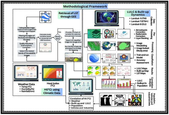
Figure 2.
Methodological framework.
2.4. Land Surface Temperature (LST) Retrieval
The Landsat data employed in this study were sourced from the United States Geological Survey (USGS), encompassing datasets from Landsat 5 and Landsat 8 Collection 2 Tier 1 Top of the Atmosphere (TOA) Reflectance [84]. These datasets were effectively employed through the Google Earth Engine (GEE) platform for the computation of the land surface temperature (LST) [85]. This study encompassed a substantial temporal range, spanning from 1990 to 2020, with images acquired annually for each year from the same collection [86,87]. The inclusion of the Landsat 5 and Landsat 8 datasets underscores the comprehensiveness and robustness of this research, offering a holistic perspective across a significant timeframe. To ensure the accuracy of the LST estimates, atmospheric correction procedures were thoroughly applied to mitigate the impact of atmospheric effects on the thermal measurements.
2.4.1. Google Earth Engine Description
Google Earth Engine (GEE), a robust geospatial cloud-computing platform [88], was utilized to process and analyze the data via its JavaScript coding interface. GEE enables researchers to access and analyze land surface temperature (LST) data derived from satellite imagery, providing valuable insights into the thermal characteristics of the Earth’s surface [89]. GEE’s capabilities allow for the retrieval and processing of large volumes of LST data, facilitating the monitoring and analysis of thermal patterns across extensive regions and time periods. GEE facilitated the retrieval of significant amounts of satellite data, enabling large-scale environmental feature monitoring and analysis [90]. This is particularly useful for studying land surface dynamics, LST, climate change impacts, and ecological processes. The platform offers tools for LST data preprocessing and a range of analytical capabilities, including statistical analysis, time series analysis, and the development of modified algorithms. Using GEE’s JavaScript coding interface, researchers can integrate LST data analysis into their broader research workflows, fostering collaboration and reproducibility within the scientific community [91,92,93,94].
2.4.2. Atmospheric Correction and Retrieval of LST
The process of calculating the LST from the Landsat imagery involved several steps, commencing with the calculation of the land surface temperature and the subsequent application of thermal conversion constants to compute the brightness temperature [95,96]. For the Landsat data, which provide top-of-atmosphere (TOA) reflectance data, atmospheric correction was necessary to ensure that the retrieved LST values accurately represented the surface temperature and were unaffected by atmospheric distortion. Therefore, the importance of atmospheric correction was acknowledged, and it was integrated it into our analysis by integrating the dark object subtraction method (DOS) [83,97,98,99]. This method (DOS) is likely the most straightforward and consistent procedure among the majority of the widely used image-based atmospheric correction procedures. The darkest pixels (assumed to have zero or minimal reflectance) in the image were identified. The minimum pixel values (dark object values) were subtracted from all the pixels to correct for atmospheric scattering. These atmospheric correction procedures ensured that the retrieval of the LST values precisely represented the surface temperature and that these values were unaffected by atmospheric distortion.
The raw Landsat data, downloaded as digital numbers, required a conversion process to obtain the spectral radiance values (Lλ), utilizing information contained in the Landsat meta header file [64,65,83].
At first, the spectral radiance of Landsat 5 TM band 6 was calculated by using Equation (1):
The formula was used to linearly rescale the DN values to radiance values. By conducting this, it was possible to convert the raw digital values obtained from the Landsat sensor into radiometrically accurate radiance values for each pixel in the image. This conversion was essential for the quantitative analysis and interpretation of the images, as it provided physically meaningful radiometric information regarding the Earth’s surface within the specific spectral band. Lλ represents the spectral radiance (W m⁻2 sr⁻1 µm⁻1), LMAXλ is the spectral radiance scaled to QCalmax (W m⁻2 sr⁻1 µm⁻1), and LMINλ denotes the spectral radiance scaled to QCalmin (W m⁻2 sr⁻1 µm⁻1). QCalmax corresponds to the maximum quantized calibrated pixel value (DN = 255) associated with LMAXλ, while the minimum quantized calibrated pixel value (DN = 0) corresponds to LMINλ. QCal refers to the quantized calibrated pixel value (DN) [100].
Similarly, in the case of Landsat 8, the digital numbers (DNs) of band 10 in Landsat 8 OLI were transformed into the spectral radiance using Equation (2):
In the context of this process, Lλ represents the top-of-atmosphere (TOA) spectral radiance measured in watts (W/(m2 sr µm)), ML represents the band-specific multiplicative rescaling feature, which was derived from the metadata, denoted as Radiance_Mult_Band_x, where ‘x’ corresponds to the band number, AL represents the band-specific additive rescaling feature from the metadata, indicated as Radiance_Add_Band_x, with ‘x’ representing the band number, and the variable QCal is associated with band 10, and it denotes the quantized and calibrated standard product pixel values (DN). TOA was determined by the equation TOA = 0.0003342 multiplied by “Band10” plus 0.1. AL is the radiance additive scaling factor for the specific band (rescaling factor from metadata).
The algorithm utilized information related to the land surface emissivity, atmospheric transmissivity, brightness temperature, and average atmospheric temperature to compute the LST as follows [101,102,103]:
In the context of this formulation, BT denotes the actual sensor brightness temperature measured in Kelvin, where ‘K1’ represents a band-specific thermal conversion constant, which was derived from the metadata and is more specifically denoted as K1_CONSTANT_BAND_x, where x corresponds to the thermal band number expressed in units of W/(m2 sr μm). Similarly, ‘K2’ stands for another band-specific thermal conversion constant from the metadata, designated as K2_CONSTANT_BAND_x, with x representing the thermal band number expressed in units of Kelvin. Additionally, Lλ signifies the spectral radiance at the sensor’s aperture, quantified in units of W/(m2 sr μm), and it is equivalently represented as TOA. To obtain the temperature results in Celsius, an adjustment was made to the radiant temperature by incorporating absolute zero, which is approximately 273.15 °C. BT = (1321.0789/Ln ((774.8853/“%TOA%”) + 1)) − 273.15.
So, finally, this formula allowed for the conversion of the calibrated radiance values from the thermal band into brightness temperatures in degrees Celsius, which could then be further processed to estimate the land surface temperature by accounting for surface emissivity effects as follows [103]:
In this equation, LST represents the land surface temperature in degrees Celsius, while ‘BT’ represents the brightness surface temperature in Kelvin, obtained directly from the thermal infrared band of the satellite imagery. The symbol λ signifies the wavelength of the emitted radiance (thermal infrared band), i.e., 10.8μm for Landsat 8 TIRs band 10. Moreover, ρ is equal to h × c/σ (1.438 × 10⁻2 mK), where ‘h’ represents Planck’s constant (6.26 × 10⁻3⁴ Js), c represents the speed of light (2.998 × 10⁸ m/s), and σ is the Boltzmann constant (1.38 × 10⁻²³ J/K). Lastly, ‘ε’ represents the land surface emissivity (ranging from 0 to 1), which accounts for the efficiency of the surface in emitting thermal radiation. In the last part of the equation, the value of −273.15 converts the LST from Kelvin to degrees Celsius.
To sum up, this formula utilizes the satellite’s brightness temperature, adjusts it according to the surface emissivity and wavelength characteristics, and then converts the outcome from Kelvin to degrees Celsius, obtaining the land surface temperature.
2.4.3. Pseudo-Code or Algorithm for LST Retrieval
Algorithm 1 provides detailed steps with numbered sequences, and each step is associated with specific actions.
| Algorithm 1 Land Surface Temperature Using GEE |
| Require Input: Landsat images set: I Ensure Output: Land Surface Temperature: T Start Initialization: 1. GEE ← Initialize Google Earth Engine 2. S ← Export shape files to GEE 3. R ← Run GEE Catalog of I (Surface Reflectance Collection) 4. ROI ← Specify region of interest (ROI) based on S 5. LST ← Set LST file export parameters Preprocessing LST: 6. SR ← Select I from R 7. ER ← Extract the ROI from I 8. M ← Create mask layer function to mask clouds, shadows, and saturated pixels 9. Apply filter on ER for additional quality assessment (optional) 10. Trange ← Mention the period or date range for the analysis 11. Apply filter and DOS method for Quality Assessment and atmospheric correction Processing LST: 12. for each image I in ER do 13. Apply filter on I for quality assessment 14. T ∞ ← Temperature value from image I 15. Tl ← Calculate Land Surface Temperature Post-processing and Visualization of LST: 16. MT ← Generate mean temperature for the whole year//Time series Analysis 17. Display MT in a chart along with Spatial Map with LST Temperature in CSV file 18. Export the results to Google Drive END |
The input data in this study were Landsat images, and the required output was to retrieve the land surface temperature. First, Google Earth Engine was loaded, the shape file was exported to Google Earth Engine by running the Google Earth Engine Catalog of Landsat Images (Surface Reflectance Collection) into Google Earth Engine, mentioning the region of interest based on the shape file along with the setting the LST file export parameters. These steps were all carried out in the initialization phase. The next step, preprocessing, involved selecting the surface reflectance data, extracting the ROI, creating a mask layer function to eliminate clouds, shadows, and saturated pixels, and optionally applying additional quality assessment filters. Atmospheric correction was performed using the DOS method within a specified date range. Processing the LST data involved iterating through each image, applying quality assessment filters, and calculating the LST. Post-processing involved generating the mean temperature for the entire year, displaying it in a chart along with a spatial map showing the annual mean temperature, and exporting the results to Google Drive.
2.5. Analyzing Climatic Data to Determine Heat Index Patterns
To calculate the heat index, weather data were collected from the regional centers of the Regional Meteorological Center (RMC) in Peshawar and the National Aeronautics and Space Administration (NASA) for all points in each year on the basis of their latitudes and longitudes. The heat index, an alternative temperature indicator, was employed to assess the impact of heat-related illnesses. Originally developed in 1978 and subsequently adopted by the U.S. National Weather Service (NWS) [104,105], the heat index is a valuable tool for evaluating climatic conditions, taking into account the combined influence of air temperature and relative humidity on human health [106]. Given that humidity plays a significant role in the body’s cooling mechanisms through evaporation and perspiration, it is crucial to consider the interplay between temperature and humidity, particularly during extreme heat events [85]. The heat index was computed using the maximum air temperature and relative humidity (as per Equation (5)) and the heat index formula established by the U.S. NWS. This calculation was implemented using the Python package “meteocalc” (version 1.10) [104].
In the above equation, ‘T’ stands for the air temperature in Fahrenheit, and ‘R’ stands for the relative humidity as a percentage (%). It is worth mentioning that the heat index (HI) values computed using this equation have a margin of error of approximately ±0.08 °C. These values were categorized into five levels, as illustrated in Table 3. However, it is important to emphasize that these classification criteria serve as broad guidelines for assessing potential health risks rather than precise indicators of specific heat-related effects or illnesses.
Table 3.
The spectrum of heat index values and the corresponding levels of concern [107,108].
Figure 3, the National Weather Service heat index chart, illustrates the relationship between temperature and humidity, providing a visual representation of perceived temperature or heat index. The color-coded heat index chart is a standard tool used by meteorological and health organizations to assess heat-related risks. It ranges from gray (normal) to red (extreme danger), providing a quick visual reference to prevent heat-related illnesses by indicating the severity of heat exposure.
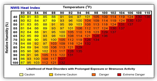
Figure 3.
National Weather Service heat index chart (source: https://www.weather.gov/ last accessed on 3 November 2023).
3. Results
This section presents the key findings of this study and is organized into the following subsections:
- 3.1. Land Use and Land Cover (LULC) Dynamics: This section analyzes the changes in land use and land cover over time, including the dynamics of built-up areas.
- 3.2. Land Surface Temperature (LST) Variations: This section examines the variations in land surface temperature using Landsat imagery from 1990 to 2020.
- 3.3. Air Quality and Industrial/Vehicular Emissions: This section analyzes the air quality data and their relationship with industrial and vehicular emissions.
- 3.4. Weather Data and Heat Index: This section investigates the variations in weather data and their effect on the heat index from 1990 to 2020. It further explores the impact of air quality and emission factors on the heat index dynamics and analyzes the correlation between the heat index and population, built-up areas, vehicles, industrial activity, and climatic data.
This comprehensive analysis provides valuable insights into the complex interplay between land use (built-up area), climate, air quality, and human activity, offering crucial information for informed decision-making and sustainable urban planning.
3.1. Land Use and Land Cover (LULC) Dynamics
This study involved the acquisition of land use and land cover (LULC) maps for the Peshawar Valley on selected days in 1990, 2000, 2010, and 2020, as shown in Figure 4, following thorough preprocessing and supervised classification. To assess the accuracy of this LULC classification, ground-truth data from Google Earth were employed, and the corresponding results are documented in Table 4. Impressively, Table 4 highlights that the classification of all LULC classes exhibited an exceptional accuracy level of nearly 90%. The classified images showcased in Figure 4 effectively capture the spatiotemporal dynamics of the LULC changes over the specified years. Furthermore, Table 5 neatly summarizes the LULC distribution for each type across the different years. A notable trend emerged in the city of Peshawar, where there was a discernible increase in built-up areas alongside a reduction in barren land from 1990 to 2020. This transformation underscores the evolving landscape of the city of Peshawar over the years, emphasizing the importance of monitoring and managing land use in urban areas.
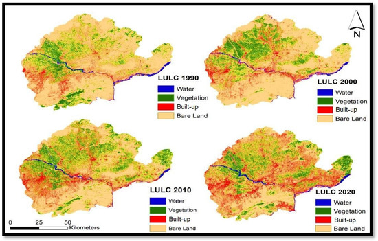
Figure 4.
Spatial patterns of land use and land cover (LULC) in Peshawar Valley.
Table 4.
Assessing the accuracy of land use classification in Peshawar Valley (%).
Table 5.
LULC assessment of Peshawar Valley.
Table 5 provides a comprehensive overview of the land use and land cover (LULC) changes over a span of three decades, from 1990 to 2020, within a specific geographic area measured in square kilometers (Sq.km) and as a percentage (%). The LULC categories studied were water bodies, vegetation area, built-up area, and bare soil. In 1990, water bodies covered 142.22 Sq.km, constituting 1.85% of the total area, and this expanded to 164.20 Sq.km (2.13%) in 2020. The vegetation area increased from 1435.36 Sq.km (18.63%) in 1990 to 1839.49 Sq.km (23.87%) in 2020. In contrast, built-up areas exhibited significant growth, rising from 489.51 Sq.km (6.35%) in 1990 to 1088.58 Sq.km (14.13%) in 2020, indicating urbanization and infrastructure development. Meanwhile, bare soil showed a gradual decline, decreasing from 5637.91 Sq.km (73.17%) in 1990 to 4612.73 Sq.km (59.87%) in 2020, possibly due to land transformation. These findings highlight the dynamic nature of the LULC changes over time, with notable shifts in urbanization, natural resource management, and environmental impacts.
These findings highlight the dynamic nature of the LULC changes over time, with notable shifts in urbanization as shown in Figure 5, natural resource management, and environmental impacts. These findings also highlight the complex interplay of human activities, environmental shifts, and land management strategies over the three-decade period, offering valuable insights for sustainable development and resource management.

Figure 5.
LULC assessment graphical representation.
Dynamics in Built-Up Areas
In the context of urban development and land use dynamics, the provided tabular data describe a compelling description of the transformation in built-up areas over the three critical decades. Commencing in 1990 with a total area of 489.51 square kilometers, urban development occupied a relatively modest 6.35% of the region. Fast-forward to the year 2000, and an undeniable change towards urbanization became apparent, as the built-up area expanded to 625.32 square kilometers, accounting for 8.11% of the total land. Over the subsequent decade, urban sprawl sustained its march, with 758.44 square kilometers now being classified as built-up areas, comprising 9.84% of the landscape by 2010. However, the data from 2020 stand as evidence for the dynamic nature of the urban growth in this study, with an expansive 1088.58 square kilometers now being observed as built-up areas, representing a considerable 14.13% of the region’s land. Notably, this period saw a surprising increase in built-up space, an expanse of 599.07 square kilometers from 1990 to 2020, marking a remarkable 7.78% change. These findings highlight the noteworthy development and increased urbanization that the region has experienced, highlighting the demanding need for maintainable urban planning and management to address the challenges and opportunities associated with such rapid development. In the context of the dynamic transformation of built-up areas in the Peshawar Valley, this research demonstrates the significant changes over the past three decades. The data analysis revealed a notable increase in built-up areas from 1990 to 2020, with a considerable growth of 599.07 square kilometers, translating to a remarkable 7.78% expansion. These data indicate an extensive shift towards urbanization and development within the region. To provide a further perspective, this expansion signifies an annual growth rate of approximately 19.969 square kilometers per year, proving the rapid pace at which the built-up environment has expanded in the Peshawar Valley, as shown in Figure 6. These findings highlight the need for comprehensive studies and sustainable urban planning to accommodate the increasing urban demand while maintaining the environmental and socio-economic dynamics of the region.
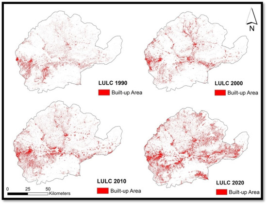
Figure 6.
Spatial patterns of built-up area dynamics in Peshawar Valley.
Table 6 provides information on the dynamics of the built-up areas in the Peshawar Valley from 1990 to 2020. Over this period, the built-up area significantly increased with a growth of 599.07 square kilometers, representing a 7.78% change. In 1990, it covered 6.35% of the total area, which grew to 14.13% by 2020, indicating significant urban expansion and development.
Table 6.
Dynamics of built-up areas in Peshawar Valley from 1990–2020.
The dynamics of the built-up areas in the Peshawar Valley, as shown in Table 7, as revealed by the data from 1990 to 2020, are interestingly interconnected with the region’s population growth. In 1990, the built-up area covered 489.51 square kilometers, while the population stood at 5.3 million. Over the successive three decades, a notable change occurred. By 2020, the built-up area expanded to 1088.58 square kilometers, indicating a substantial 7.78% increase. Simultaneously, the population grew rapidly from 5.3 million in 1990 to a surprising 12.6 million in 2020, representing an unpredictable growth of 7.04 million individuals. This extensive change is associated with an annual increase of approximately 234,874 people. The association between the population and built-up area dynamics underscores the deep influence of urbanization and demographic shifts within the Peshawar Valley as shown in the Figure 7.
Table 7.
Population from 1990–2020 in Peshawar Valley based on population census.
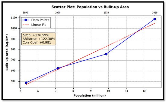
Figure 7.
Graphical representation of population and built-up area dynamics in Peshawar Valley.
This synchronous growth in population and urban footprint suggests a close correlation between demographic dynamics and urban expansion in the Peshawar Valley. It is important to recognize this interaction for effective urban planning and developing sustainable development strategies moving forward. This study underscores the need for practical measures to manage urban growth in a manner that ensures the well-being and quality of life for the growing population in the Peshawar Valley.
The population projection and the inter-censual growth rates (1981–2023) were applied to the district projections using Equation (6):
where Po represents the population from the initial census, P1 represents the population from the latest census, r represents the growth rate, and n is the time interval (in years) between the two censuses.
P1 = Po (1 + r)n/100
Figure 8 represents the data for the years 1990, 2000, 2010, and 2020, showing the population and built-up area percentages. These percentages were measured in terms of the change from 1990 to 2020, providing insights into the growth and development over this three-decade period. In 1990, the population was 17.09%, and the built-up area was 15.24%. By 2000, the population increased to 21.85%, and the built-up area expanded to 20.46%. In 2010, the population continued to grow to 26.52%, while the built-up area also increased to 28.26%. By the year 2020, the built-up area expanded to 36.18%, while the population reached 37.95%. Over the span of 30 years, as indicated by these results, it is very clear that there has been substantial growth in both the population and built-up area. Over the span of three decades, the population effectively almost doubled, with a remarkable growth of 20.86%. Likewise, the built-up area demonstrated considerable expansion, registering a growth of 20.94% during the same period. These results clearly show a significant trend of the urbanization sprawl and population growth over the years, consequently leading to a notable expansion in the built-up area. Considering the implications of this growth is crucial in terms of various aspects, such as infrastructure, land use management, and environmental sustainability, as these transformations carry substantial consequences for the region.

Figure 8.
Population and built-up area projection comparison in percentage.
3.2. Land Surface Temperature (LST) Variations using Landsat Imagery from 1990–2020
The computation of the land surface temperature (LST) variation for the Peshawar Valley for the years in the 1990s, 2000s, 2010s, and 2020s was examined following the procedure detailed in Section 2.4 of the methodology, as shown in Figure 2. The comprehensive examination of the LST variations in the Peshawar Valley over three decades (1990–2020) unveiled a notable temperature fluctuation, as brightly shown in Figure 9. In the 1990s, the maximum recorded LST was 26.28 °C, which actually indicates the maximum mean LST for the whole year. Similarly, in the 2000s, the LST values showed a gradual rise in temperature, reaching a maximum of 27.09 °C. Subsequently, in the 2010s, and the maximum LST reached 29.49 °C. Significantly, in the 2020s, the trend continued, and the maximum LST finally reached 30.30 °C. These findings show a consistent rising trend in the LST over the years, signaling an apparent increase in temperature within the Peshawar Valley. These findings also highlight the overall warming pattern in the region. These fluctuations in temperature serve as a critical indicator of climate change and could have substantial consequences for the environment and human activities within the Peshawar Valley.
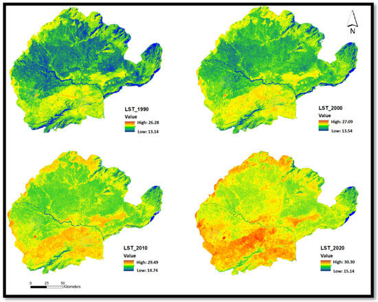
Figure 9.
Mapping land surface temperature (LST) patterns in degrees Celsius.
3.3. Analysis of Air Quality and Relationship with Industrial and Vehicular Emissions
Over the observed years, the number of registered vehicles demonstrated a significant increase from 1990 to 2020, showcasing a substantial growth in vehicular activity. Furthermore, the population and urbanization also witnessed notable expansion during this period. Additionally, the number of running industries demonstrated a steady rise, further indicating an upward trend in industrial activity. These trends collectively underscore the substantial influence of transportation, industry, population, and urbanization on the region’s air quality.
Table 8 demonstrates that over the observed years, the number of registered vehicles increased significantly from 0.171 million to 1.364 million in 2020, indicating substantial vehicular growth. Similarly, the number of running industries also steadily rose, increasing from 327 in 1990 to 1155 in 2020, showing an upward trend in industrial activity. These trends highlight the growing impact of transportation and industry on the region, as shown in Figure 10.
Table 8.
Number of registered vehicles and running industries (1990s–2020).

Figure 10.
Spatial distribution of registered vehicles and running industries (1990’s–2020).
Particulate matter with a diameter of 2.5 micrometers or even smaller, commonly known as PM 2.5, can arise as a byproduct of emissions originating from vehicles and various industrial sources. PM 2.5 comprises microscopic solid particles or liquid droplets floating in the air, and it encompasses different elements such as dust, soot, organic materials, and metals. PM 2.5 is released into the atmosphere through vehicles as they burn fossil fuels, particularly in engines that lack advanced pollution-mitigation technologies. This involves the emission of particles from exhaust pipes as well as wear from brakes and tires. Similarly, industries also discharge PM 2.5 through activities like manufacturing, construction, and the functioning of power plants. Operations of industries can also generate dust and smoke that can contribute to heightened levels of PM 2.5 in the atmosphere. Hence, both vehicles and industries emerge as notable sources of PM 2.5 pollution. The data shown in Figure 11, representing the annual PM 2.5 levels from 2005 to 2020, indicate variations in the air quality in the studied area. The increase in both the number of registered vehicles and the number of running industries in this context is crucial because it can contribute to elevating the levels of air pollution, including PM 2.5. These trends suggest a potential connection between the levels of air pollution, particularly PM 2.5, and the expansion of running industries and vehicles within the Peshawar Valley. Therefore, it is very important to regulate and control the measurement of these emissions to mitigate their influence on air quality and public health.

Figure 11.
Observed annual mean of PM 2.5, obtained via CAMS data.
The different colors in the Table 9 represent the air quality categories for PM 2.5 concentration, which help to quickly and visually identify the air quality level. This categorization is necessary for easy and immediate comprehension of the air quality status, facilitating informed decision-making and prompt action when necessary.
Table 9.
Categories for the 24 h moving average concentrations of PM 2.5 in the European Air Quality Index (EAQI) [109].
Figure 12 shows the mean aerosol optical depth (AOD), which provides a general assessment of the proportion of various aerosols. The AOD (aerosol optical depth) values and the proportions of various aerosols provide insights into the composition of particulate matter in the atmosphere. In the context of urbanization, transportation, and industrial data, organic aerosols (45.95%) could be related to emissions from various sources, including vehicles and industries. Organic aerosols often contain carbon compounds and can originate from the incomplete combustion of fossil fuels, which is common in urban areas with high vehicular traffic and industrial activity. Black carbon (3.09%) is a component of fine particulate matter that is primarily emitted from the combustion of fossil fuels, especially diesel engines. This aerosol component can be linked to vehicular emissions, particularly in urban areas with heavy traffic. Sulfate aerosols (32.38%) are often associated with industrial processes and power generation. Urban and industrial areas with significant sulfur dioxide (SO2) emissions can contribute to the formation of sulfate aerosols. Dust (17.68%) may be influenced by land use changes associated with urbanization, such as construction and road development. Additionally, dust aerosols can be generated in arid regions or areas with minimal vegetation. Other aerosols (0.94%) may include various aerosols of different origins. Depending on the specific composition, these aerosols can be associated with diverse urban, transportation, or industrial activities.
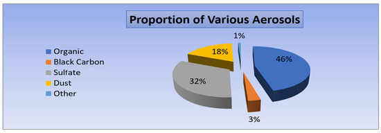
Figure 12.
Breakdown of aerosols observed at 550 through CAMS.
Understanding the proportions of these aerosols in the AOD values is essential for assessing air quality and identifying potential sources of pollution in urban and industrial regions. The data suggest that multiple factors, including urbanization, transportation, and industrial emissions, can contribute to the composition of aerosols in the atmosphere, ultimately affecting air quality and public health.
The source apportionment data for air pollution shown in Figure 13 can be explained in the context of various factors, including vehicles, industries, population, and urbanization. The highest contributor to air pollution in these data was transportation, with a value of 58.46%. This indicates that a significant portion of the air pollution was linked to vehicle emissions. The increase in the number of vehicles, especially in urban areas, as a result of population growth and urbanization can lead to higher emissions of pollutants. Industrial activities, which accounted for 6.58%, contribute to air pollution, but their share was relatively small compared to transportation emissions. However, industries were still a noteworthy source of pollutants in the study area, and their impact may be more pronounced in industrial zones within urban areas. Waste burning (4.10%) contributes to air pollution, and this source can be associated with both domestic and commercial activities within urban regions. As urbanization occurs, the generation of waste can increase, leading to more burning activities. Domestic (11.66%) sources include household activities like cooking and heating, which can produce pollutants. As urban populations grow, the number of households and domestic activities also increases, potentially elevating emissions from these sources. Commercial (1.49%) emissions, including those in business districts, contributed to air pollution to a lesser extent within the study area. However, with urbanization, there is often an expansion of commercial areas and businesses, which may lead to a proportionate increase in emissions. Dust (17.67%) emissions are strongly linked to urbanization and construction activities. As urban areas expand and undergo development, there is more construction, road building, and land disturbance, all of which can result in the release of dust into the air. In short, source apportionment data underscore the complex interplay of various factors in urban areas. Increases in population, urbanization, and industrialization lead to more vehicles, industrial emissions, domestic and commercial activities, and construction, all of which can collectively contribute to air pollution. Understanding the sources of pollution is crucial for implementing effective strategies for mitigating air quality issues and improving public health.

Figure 13.
Source apportionment of air pollution.
3.4. Variations in Weather Data and Effect on Heat Index from 1990–2020
The data provided in Table 10 cover three decades, showing the monthly variations in climate parameters from 1991 to 2020 in the Peshawar Valley, including the maximum temperature (°C), minimum temperature (°C), mean relative humidity (%), mean rainfall (mm), and calculated heat index (HI) values. The dataset compilation involved the collection and analysis of monthly values for each parameter for all the points from the month of May to September. Calculating the mean temperature involved the process of averaging the daily temperature recorded throughout each month, and a similar approach was used to compute the mean relative humidity, which was obtained from the monthly humidity values. The mean rainfall was determined by taking the average of the monthly precipitation values. The extensive dataset provides detailed insight into the climatic conditions in the Peshawar Valley throughout the years, which can enable researchers and meteorologists to monitor the weather, including trends, changing patterns, and potential implications for both the local environment and the well-being of the community. Remarkably, the data revealed a substantial variation in the temperature, humidity, and heat index values throughout the years.
Table 10.
Climatic data and heat index (HI) values for three decades (1990–2020).
Table 10 provides a detailed summary of the climatic data and heat index (HI) values spanning the three decades (1990–2000, 2001–2010, and 2011–2020), presenting insights into the fundamental meteorological parameters. The presented dataset incorporates the maximum temperature, minimum temperature, relative humidity (RH) as a percentage, rainfall (RF) measured in millimeters, and the corresponding calculated values of the heat index (HI).
The information presented in Table 10 encapsulates the fascinating trends in the climatic conditions across the three decades. The chronological progression highlights a notable pattern in the maximum and minimum temperature, relative humidity, rainfall, and the substantial heat index.
Notably, during the specified decades, a discernible decrease was observed in both the maximum as well as the minimum temperature over the years. For the initial decade 1991–2000, the maximum temperature was recorded as 42.94 °C, with a corresponding minimum temperature of 19.009 °C. In the subsequent decade (2001–2010), the maximum temperature slightly decreased to 42.01 °C, while the minimum temperature showed a small increase, reaching 19.431 °C. Eventually, during the last decade (2011–2020), the maximum temperature continued to decrease, reaching 40.86 °C, while the minimum temperature experienced a decline, reaching 19.19 °C.
However, a noticeable aspect of the data is the escalating trend observed in the heat index values. Contrastingly, despite the decreasing trend in the maximum temperature, the HI values consistently continued to rise. In the 1991–2000 decade, the maximum HI value reached at 50.54 °C, subsequently progressing to 53.19 °C in the following decade of 2001–2010, and in the most recent decade of 2001–2020, it further intensified to 55.48 °C. The HI over the last three decades is of huge concern, as the HI escalated 5 °C, surging from 50.54 °C to 55.48 °C. This observation can be correlated with the escalating levels of the relative humidity (RH). In the 1990s, the RH stood at 31.789%, after which there was a clear rise, with the RH increasing to 39.308% from 2001 to 2010, and there was a similar subsequent increase to 47.40% from 2011–2020. Correspondingly, the RF recorded a value of 27.366 mm from 1991–2000, subsequently showing an upward trend in the RF pattern, where it stood at 39.597 mm from 2001–2010; similarly, in the last decade of 2011–2020, the RF was recorded as 69.71 mm. The variations and increases in the RF patterns serve as the contributing factors to the increased RH level. Increases in humidity levels exert a crucial influence on the heat index, highlighting the significance of taking not only increasing temperatures but also humidity into account when assessing the real-world consequences of climate change on day-to-day living conditions.
The upward trend in the heat index values indicates a trend towards more uncomfortable climatic conditions, raising significant concerns for both the environment and potential health risks to human well-being. Extreme heat can strain the human body’s ability to cool itself, leading to heat stress, heat exhaustion, and potentially life-threatening conditions like heat stroke. The likelihood of experiencing heat stroke is substantial if the HI is above 54 °C, as stated in Table 3. The increase in the HI value reflects an intensification of heat-related challenges, emphasizing the urgency of adaptive measures, public health interventions, and sustainable practices to mitigate the adverse impacts of climate change on both the human societies and the natural environment.
3.4.1. Heat Index Dynamics: Exploring the Impact of Air Quality and Emission Factors
The heat index (HI) is influenced by critical factors, and the preceding sections presented crucial insights into these influences through the provided data. Highlighting the increasing influence of transportation and industrial emissions on the region’s environmental dynamics, the substantial surge in transportation and the consistent growth in industrial operations from 1990 to 2020 stand out prominently. These emissions, including an array of both heat-trapping gases and PM 2.5, play a crucial role in contributing to the escalation in the heat index. Moreover, the existence of PM 2.5 produced by both transportation and industrial operations has a fundamental role in shaping the heat index. The absorption and re-radiation of heat affects temperature levels and are affected by microscopic airborne particles present in the air, particularly those found in PM 2.5. The variations in the yearly PM 2.5 levels are correlated with vehicular and industrial emissions, which also indicates a possible influence on the heat index. Moreover, the composition of different aerosols, as shown in Figure 14, is reflected by the involved interaction of urbanization, transportation, and in various industrial activities. Organic aerosols such as black carbon and sulfate aerosols are components that are capable of interacting with solar radiation, modifying heat levels within the urban environment, and they consequently play a crucial role in influencing the heat index. Lastly, the distribution of the source data unveils the involved relationship between emission sources and urbanization. The crucial role of transportation in air pollution, propelled by population growth and urbanization, underscores its influence on the local temperature and heat index. On the other hand, industrial activities, along with other contributing sources, also play a distinctive role that contributes to jointly influencing the thermal dynamics of the region.
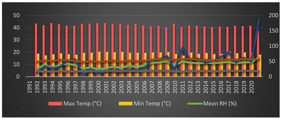
Figure 14.
Graphical visualization of climatic data and heat index (HI) (1990s–2020).
In a nutshell, the data regarding the air quality, emission sources, and their interconnections highlight the complex factors that influence the heat index. Understanding these factors is crucial for effective urban planning and for creating strategies to adapt to climate change. The goal is to minimize the influence of life-threatening heat and to improve the overall quality of life in urban areas. To be successful in this goal, metropolitan regions can adopt strategies like expanding green spaces to improve the urban environment and improving infrastructure designed for greater resilience to heat-related challenges, and strategic planning for sustainable urban development is essential for fostering long-term environmental and community well-being. Additionally, public awareness campaigns and promoting community engagement can empower residents to adopt practices that can contribute to minimizing the impact of extreme heat and contribute to a more sustainable urban environment.
3.4.2. Correlation between HI and Population, Built-Up Area, Vehicle, Industrial, and Climatic Data
The HI was strongly positively correlated with built-up area (0.98), population (0.99), vehicles, and running industries (0.97), as presented in Figure 15. This implies that as these factors increase, the heat index significantly increases. Urbanization, population density, and vehicular activity contribute to higher heat index values. The heat index (HI) increases primarily due to a combination of several key factors, including urbanization, population growth, and the rising number of registered vehicles. Here is an in-depth discussion of how these elements affect the rise in the HI.

Figure 15.
Correlation between heat index and other factors (population, built-up area, vehicles, and industries).
Population Growth: As the population of a region grows, urban areas see a rise in population density, and a higher population density frequently results in greater human activity, consumption of energy, and heat production. As a result, local temperatures rise, and the heat index is elevated.
Urbanization and Built-Up Areas: Built-up areas featuring heat-retaining surfaces like concrete and asphalt grow in number as areas undergo substantial growth and become more urbanized. Urbanization contributes to the formation of “urban heat islands”, marked by notably elevated temperatures and heat index (HI) values in contrast to the surrounding rural areas, and excessive HI values are the consequence of these heat islands.
Number of Registered Vehicles and Industries: The rise in the number of registered vehicles on the road and the number of running industries is linked to higher heat and emissions produced by traffic and industries. Heat-trapping gases are emitted by transportation and industrial operations, which raise the temperature in urban areas and, in turn, the heat index.
In a nutshell, the combined effects of population expansion, urbanization, and increasing numbers of vehicles and industrial activities cause the heat index to rise. These factors contribute to the formation of localized heat pockets in urban regions, raising the heat index levels. In order to mitigate the adverse consequences of excessive heat while improving urban living conditions, it is essential to take these aspects into consideration when developing urban planning and climate adaptation methods.
Furthermore, from 1990 to 2020, the heat index surged despite trends indicating a drop in air temperature, an upward trend in relative humidity, and a concurrent increase in rainfall. This indicates that the higher heat index values during this period were mostly caused by humidity, which is influenced by rainfall patterns. The substantial rise in the relative humidity brought on by more rainfall can be partially attributed to the observed increase in the HI. Moreover, there was an obvious impact of urbanization expansion, which is defined as the spread of impermeable surfaces like cement and asphalt. After the occurrence of rainfall, these surfaces delay the natural drainage process, causing water to remain there for prolonged periods following rainfall storms. The local relative humidity rises as a result of this water retention effect, which raises the heat index even more in urban areas. When evaluating the heat index and its related consequences in the context of urban environments, it is important to take into consideration a variety of factors due to the complex connections between these climatic and urbanization aspects.
4. Discussion
Urbanization is a global phenomenon with well-documented environmental consequences [44]. This study investigated the interconnected impacts of population expansion, land use and land cover (built-up areas) dynamics, air quality variations, and climatic conditions on the heat index (HI) within the Peshawar Valley over a three-decade period (1990–2020). Our findings corroborate existing knowledge regarding the influence of urbanization on LULC changes and rising temperatures [6]. However, this study extends this knowledge base by analyzing the combined effect of these factors on the HI, a crucial indicator of thermal comfort and potential health risks. The findings of this study presented an in-depth understanding of how population, urbanization, anthropogenic activities, and climatic variations have different consequences that influence the environment.
Prior research has established a connection between urban sprawl and increased built-up areas and altered LULC patterns [63]. This study aligns with these findings, demonstrating a statistically significant expansion of built-up areas in the Peshawar Valley coinciding with population growth. Analyzing the changes in population and the transformation in LULC highlights the significant infrastructure developments and urbanization in the Peshawar Valley. Notably, from 1990 to 2020, there was a significant increase in population, from 5.3 million to 12.6 million, while the built-up area increased from 489.51 km2 to 1088.58 km2, as shown in Figure 4 and Figure 6. The substantial increase in the built-up area was necessitated due to the large of number of the people who migrated to the Khyber Pakhtunkhwa Province during the US–Afghan war and due to severe instability in the region between 2000–2005 [59,110]. This surge is closely linked to the significant increase in population, highlighting the mutual connection between the population and the expansion in the built-up region during the same period, as shown in Figure 7.
Variations in the LST are caused by changes in LULC, and our results are consistent with the established understanding that variations in LULC cause variations in the LST because different LULC patterns possess their own unique characteristics of reflectance and transpiration of water [111]. The LST results shown in Figure 9 indicate that there was a consistent increase in the temperature over the 30 years studied, presenting a warming trend in the Peshawar Valley. The temperature showed a consistent increase and recorded a higher increase in 2020 compared to the 1990s. The increase in temperature could have been caused by the increasing demand for artificial materials, such as asphalt and concrete, for the expansion of the built-up regions [6]. The results shown in Figure 6 indicate that built-up region expanded over the three decades, thus effectively influencing the LST.
Furthermore, this study builds upon existing knowledge concerning the negative environmental consequences of rapid urbanization, particularly air quality deterioration due to various anthropogenic activities, including biogeochemical and biochemical processes [44]. Pakistan has witnessed a rapid increase in vehicular traffic on its roads and industrial expansion [45], and our findings reveal a clear correlation between population growth and increased vehicular traffic and industrial activity within the Peshawar Valley, aligning with observations from other studies on rapid urbanization in developing countries. Similarly, Figure 10 highlights a significant increase in vehicular traffic on the roads and also a gradual increase in industrialization in the Peshawar Valley, indicating that different biochemical mechanisms and the emission of various gases into the atmosphere have serious consequences for the environment, especially air quality. This aligns with established knowledge that these anthropogenic activities are major contributors to air pollution, particularly fine particulate matter (PM 2.5) emissions, significantly impacting air quality [45,48]. The observed “Very Poor” and “Extremely Poor” air quality categories in the Peshawar Valley, as measured by the European Air Quality Index (EAQI) [109] shown in Table 9, highlight the critical need to address air pollution in the region, as evidenced by the various aerosol compositions depicted in Figure 12 and the variations in the PM 2.5 levels shown in Figure 11, indicating the complex interplay between urbanization, transportation, and industrial activities influencing the region’s air quality and contributing to climate change.
Temperature studies in urban areas are vital for assessing thermal comfort, energy consumption, and emissions of greenhouse gases and pollutants, which contribute to global warming alongside secondary effects on the local climate [12,13,14]. The climatic data provided in Table 10 offer a comprehensive overview of the temperature trends, rainfall patterns, relative humidity, and heat index data spanning the three decades in the Peshawar Valley. The analysis depicted in Figure 14 reveals substantial disruptions in rainfall patterns over the last decade, resulting in higher relative humidity (RH) levels, contributing to elevated heat index (HI) values. These trends indicate a shift towards increasingly uncomfortable climatic conditions, posing potential health risks for residents in the region, particularly as HI values exceeding 54 degrees’ Celsius fall into the category of “Extreme Danger”, presenting a substantial risk of heat stroke [85,106]. Additionally, rapid increases in urbanization generate enormous challenges, influencing local and regional climatic conditions [44]. Furthermore, the expansion of built-up areas over the past three decades has exacerbated the HI levels, potentially driven by an increased demand for artificial materials like asphalt and concrete, which alter land use and land cover (LULC) patterns and contribute to higher temperatures in urban areas due to their unique reflectance and transpiration characteristics [6,111]. Our study highlights the significant role of urbanization, air quality deterioration, and anthropogenic activities such as increased traffic and industrial emissions in shaping the HI within the region. We observed a strong correlation between the HI and various factors, including changes in climatic data, population growth, expansion of built-up areas, and intensification of traffic and industrial activity. This correlation underscores the intricate relationship among these factors, influencing the heat index of the Peshawar Valley. These findings corroborate recent research emphasizing the complex interplay between urbanization, altered LULC patterns, and local climatic conditions, ultimately impacting thermal comfort and potentially elevating health risks associated with heat-related illnesses [85,106].
This study also offers a unique contribution to the existing body of research as follows:
Measuring the interconnected effects of population expansion, LULC dynamics, air quality variations, and climatic conditions on the HI within a specific urban setting (the Peshawar Valley).
- Highlighting the importance of the HI as a metric for understanding the combined effects of urbanization and climate change on human health and thermal comfort.
- Providing valuable data for urban planners and policymakers in developing sustainable strategies to mitigate the negative environmental consequences of urbanization in the Peshawar Valley.
These insights can inform the development of targeted interventions such as promoting green infrastructure projects, creating walkable and cyclable urban environments to reduce reliance on private vehicles, and implementing stricter regulations on industrial emissions.
5. Conclusions
In conclusion, the in-depth analysis presented in “Urbanization, Climate Change, and Demographic Shifts: A Comprehensive Investigation of the Peshawar Valley” revealed a wide range of interlinked findings. Collectively, these findings indicate the significant consequences of rapid urbanization, a shift in demographics, and climate change in the region as a whole. Over the three-decade study period, rapid urbanization was witnessed within the Peshawar Valley. The population increased significantly from 5.3 million in 1990 to a surprising 12.6 million in 2020. The built-up areas also recorded a considerable increase, rising from 489.51 square kilometers to 1088.58 square kilometers. The increase in the population within the region, driven by a number of factors, has contributed to a large number of anthropogenic activities, including the propagation of transportation and the establishment of industries. These developments have left a noticeable effect on the environment, affecting air quality standards. The rising values of the heat index (HI) indicate the presence of an urban heat island effect within the region. This phenomenon not only has consequences on the environment but also affects the public and psychological health of the residents.
Furthermore, the shifting climate of the Peshawar Valley, as evidenced by the steady rise in the land surface temperature (LST) and heat index (HI) readings, provides greater clarity as to the complex relationship between urbanization and climate change. In particular, over the studied decades, the land surface temperature (LST) has progressively risen. The most extreme temperature ever recorded rose from 28.11 °C in 1990 to 30.30 °C in 2020, reflecting the consequences of these changes on the natural environment. The heat index, which has a strong correlation with population, built-up areas, and the number of vehicles and industries, witnessed a substantial rise. In the final ten years of the study, the HI reached a maximum mean heat index value of 54.48 °C. This rise brings attention to the area’s increasing heat stress and highlights the combined effects of increasing urbanization, increasing population, and the urban heat island effect. The region’s rising degree of heat stress is highlighted by the escalating surge, which is a sign of the combined effects of increasing urbanization, population growth, and the urban heat island effect. Together, these results emphasize the intertwined challenges and opportunities brought about by the complicated dynamics of urbanization, climate change, and demographic shifts in the Peshawar Valley. To address these complex issues comprehensively, integrated strategies aimed at preserving the environment, enhancing public health, and ensuring the resilience of the community in the face of evolving urban and climatic forces are imperative.
The anticipated future scenarios suggest that the Peshawar Valley is likely to encounter significant environmental challenges. However, the outcomes of this study unveil encouraging trajectories for the region, signaling a pathway to enhancing living conditions amid urban expansion. The examination of the LULC dynamics underscores the substantial urbanization and infrastructure development, exemplified by a noteworthy expansion in the built-up area in the region. This highlights the immediate need for sustainable urban planning and adept land use management to meet the escalating urban demands while upholding the delicate equilibrium of environmental and socio-economic dynamics. Concurrently, the land surface temperature (LST) analysis discloses a consistent warming trend, indicating the broader implications of climate change. The observed increase in both the LST and heat index (HI) over the years underscores the pressing significance of considering not only temperature but also humidity when evaluating the implications of climate change on daily life. The intricate relationships between air quality, industrial and vehicular emissions, climatic conditions, and their collective influence on the HI serve as pivotal considerations for policymakers and environmentalists. This research provides indispensable information for formulating targeted greening strategies tailored to the unique dynamics of the Peshawar Valley, aiming to proactively mitigate potential eco-environmental threats and foster sustainable urban ecosystems for its residents.
Overall, this study’s findings contribute to the existing literature by elucidating the interconnected impacts of population growth, urbanization, industrialization, and climatic variations on the environmental dynamics within the Peshawar Valley. By linking the empirical results to broader theoretical frameworks, this research underscores the importance of holistic approaches in understanding and addressing the complex challenges posed by urbanization and climate change.
It is important to acknowledge that this study has limitations. This study acknowledges the limitations in terms of data availability for assessing chronic health impacts associated with environmental factors in the Peshawar Valley. While we aimed to analyze the connection between environmental changes and human health, obtaining reliable data proved challenging.
In future, research can address these limitations and expand upon the current knowledge, investigating the long-term health impacts associated with chronic exposure to elevated HI levels in the Peshawar Valley. This could involve collaborating with public health researchers to conduct epidemiological studies, potentially analyzing existing hospital data on heatstroke and other environment-related illnesses.
The solutions to climate change require a multi-faceted approach, including transitioning to renewable energy sources by shifting away from fossil fuels and towards renewable energy sources like solar and wind power, increasing energy efficiency by improving the energy efficiency of buildings, transportation, and industry, electrifying transportation through switching to electric vehicles and public transportation, developing carbon capture and storage technologies that can capture and store carbon dioxide emissions, implementing sustainable land use practices such as sustainable agriculture, reforestation, and conservation efforts, and collaborating globally through international cooperation to address the causes and effects of climate change. Additionally, developing and evaluating adaptation strategies to improve thermal comfort in urban environments, such as incorporating cool roof materials and urban greening initiatives, can be an effective approach. Field experiments or simulations can be employed to assess the effectiveness of these strategies in mitigating the impacts of climate change and urban heat islands.
Author Contributions
Conceptualization, Muhammad Farooq Hussain, Xiaoliang Meng, Syed Fahim Shah and Muhammad Asif Hussain; methodology, Muhammad Farooq Hussain and Xiaoliang Meng; software, Muhammad Farooq Hussain; writing—original draft preparation, Muhammad Farooq Hussain; writing—review and editing, Muhammad Farooq Hussain and Xiaoliang Meng; formal analysis, Muhammad Farooq Hussain and Xiaoliang Meng; data curation, Muhammad Farooq Hussain; supervision, Xiaoliang Meng. All authors have read and agreed to the published version of the manuscript.
Funding
This research was funded by the National Natural Science Foundation of China, grant number 41971352.
Data Availability Statement
The datasets used and/or analyzed during the current study are available from the first author upon reasonable request.
Acknowledgments
Our sincere appreciation is extended to the National Natural Science Foundation for their generous financial support, significantly contributing to the academic advancement of this research. We express gratitude to the Peshawar Clean Air Alliance and the entire team. Their dedication to improving air quality resonates with the broader vision of this study—a vision aspiring to witness the transformation of Peshawar Valley’s mountains and to elevate the academic standing of Peshawar and Khyber Pakhtunkhwa. This acknowledgment underscores the efforts and commitment to fostering positive academic contributions in the realm of environmental research.
Conflicts of Interest
The authors declare no conflicts of interest.
References
- Ramzan, M.; Saqib, Z.A.; Hussain, E.; Khan, J.A.; Nazir, A.; Dasti, M.Y.S.; Ali, S.; Niazi, N.K. Remote sensing-based prediction of temporal changes in land surface temperature and land use-land cover (LULC) in urban environments. Land 2022, 11, 1610. [Google Scholar] [CrossRef]
- Georgati, M.; Hansen, H.S.; Keßler, C. Random Forest Variable Importance Measures for Spatial Dynamics: Case Studies from Urban Demography. ISPRS Int. J. Geo-Inf. 2023, 12, 460. [Google Scholar] [CrossRef]
- Gu, D.; Andreev, K.; Dupre, M.E. Major trends in population growth around the world. China CDC Wkly. 2021, 3, 604. [Google Scholar] [CrossRef]
- Selod, H.; Shilpi, F. Rural-urban migration in developing countries: Lessons from the literature. Reg. Sci. Urban Econ. 2021, 91, 103713. [Google Scholar] [CrossRef]
- Zhai, H.; Lv, C.; Liu, W.; Yang, C.; Fan, D.; Wang, Z.; Guan, Q. Understanding spatio-temporal patterns of land use/land cover change under urbanization in Wuhan, China, 2000–2019. Remote Sens. 2021, 13, 3331. [Google Scholar] [CrossRef]
- Mumtaz, F.; Tao, Y.; de Leeuw, G.; Zhao, L.; Fan, C.; Elnashar, A.; Bashir, B.; Wang, G.; Li, L.; Naeem, S.; et al. Modeling spatio-temporal land transformation and its associated impacts on land surface temperature (LST). Remote Sens. 2020, 12, 2987. [Google Scholar] [CrossRef]
- Güneralp, B.; Zhou, Y.; Ürge-Vorsatz, D.; Gupta, M.; Yu, S.; Patel, P.L.; Fragkias, M.; Li, X.; Seto, K.C. Global scenarios of urban density and its impacts on building energy use through 2050. Proc. Natl. Acad. Sci. USA 2017, 114, 8945–8950. [Google Scholar] [CrossRef] [PubMed]
- Ziter, C.D.; Pedersen, E.J.; Kucharik, C.J.; Turner, M.G. Scale-Dependent Interactions between Tree Canopy Cover and Impervious Surfaces Reduce Daytime Urban Heat during Summer. Proc. Natl. Acad. Sci. USA 2019, 116, 7575–7580. [Google Scholar] [CrossRef]
- Alexander, C. Influence of the Proportion, Height and Proximity of Vegetation and Buildings on Urban Land Surface Temperature. Int. J. Appl. Earth Obs. Geoinf. 2021, 95, 102265. [Google Scholar] [CrossRef]
- Wemegah, C.S.; Yamba, E.I.; Aryee, J.N.A.; Sam, F.; Amekudzi, L.K. Assessment of Urban Heat Island Warming in the Greater Accra Region. Sci. Afr. 2020, 8, e00426. [Google Scholar] [CrossRef]
- Yang, J.; Zhan, Y.; Xiao, X.; Xia, J.C.; Sun, W.; Li, X. Investigating the Diversity of Land Surface Temperature Characteristics in Different Scale Cities Based on Local Climate Zones. Urban Clim. 2020, 34, 100700. [Google Scholar] [CrossRef]
- Hussain, M.; Liu, G.; Yousaf, B.; Ahmed, R.; Uzma, F.; Ali, M.U.; Ullah, H.; Butt, A.R. Regional and sectoral assessment on climate-change in Pakistan: Social norms and indigenous perceptions on climate-change adaptation and mitigation in relation to global context. J. Clean. Prod. 2018, 200, 791–808. [Google Scholar] [CrossRef]
- Swamy, G.S.; Nagendra, S.M.; Schlink, U. Impact of Urban Heat Island on Meteorology and Air Quality at Microenvironments. J. Air Waste Manag. Assoc. 2020, 70, 876–891. [Google Scholar] [CrossRef]
- Fu, P.; Weng, Q. A Time Series Analysis of Urbanization Induced Land Use and Land Cover Change and Its Impact on Land Surface Temperature with Landsat Imagery. Remote Sens. Environ. 2016, 175, 205–214. [Google Scholar] [CrossRef]
- Wang, H.; Liu, X.; Zhao, C.; Chang, Y.; Liu, Y.; Zang, F. Spatial-temporal pattern analysis of landscape ecological risk assessment based on land use/land cover change in Baishuijiang National nature reserve in Gansu Province, China. Ecol. Indic. 2021, 124, 107454. [Google Scholar] [CrossRef]
- Xiang, T.; Meng, X.; Wang, X.; Xiong, J.; Xu, Z. Spatiotemporal Changes and Driving Factors of Ecosystem Health in the Qinling-Daba Mountains. ISPRS Int. J. Geo-Inf. 2022, 11, 600. [Google Scholar] [CrossRef]
- He, W.; Zhang, L.; Yuan, C. Future air temperature projection in high-density tropical cities based on global climate change and urbanization–a study in Singapore. Urban Clim. 2022, 42, 101115. [Google Scholar] [CrossRef]
- Tumse, S.; Bilgili, M.; Sekertekin, A.; Ünal, Ş.; Sahin, B. Comparison and evaluation of machine learning approaches for estimating heat index map in Türkiye. Neural Comput. Appl. 2023, 35, 15721–15742. [Google Scholar] [CrossRef]
- Ghalhari, G.F.; Dehghan, S.F.; Shakeri, F.; Ghanadzadeh, M.J.; Asghari, M. Assessing the monthly changes of heat stress indices in outdoor environment during a 15-year period: Case of study in a dry and warm climate. Urban Clim. 2020, 31, 100538. [Google Scholar] [CrossRef]
- Zune, M.; Rodrigues, L.; Gillott, M. The vulnerability of homes to overheating in Myanmar today and in the future: A heat index analysis of measured and simulated data. Energy Build. 2020, 223, 110201. [Google Scholar] [CrossRef]
- Aksu, O.; Iban, M.C. Considerations on the Land Management System Approach in Turkey by the Experiences of a Case Study. Surv. Rev. 2019, 51, 87–96. [Google Scholar] [CrossRef]
- Hill, A.C.; Laugier, E.J.; Casana, J. Archaeological remote sensing using multi-temporal, drone-acquired thermal and Near Infrared (NIR) Imagery: A case study at the Enfield Shaker Village, New Hampshire. Remote Sens. 2020, 12, 690. [Google Scholar] [CrossRef]
- Shao, Z.; Wu, W.; Li, D. Spatio-temporal-spectral observation model for urban remote sensing. Geo-Spat. Inf. Sci. 2021, 24, 372–386. [Google Scholar] [CrossRef]
- Kafy, A.-A.; Naim, N.H.; Khan, M.H.H.; Islam, M.A.; Al Rakib, A.; Al-Faisal, A.; Sarker, M.H.S. Prediction of Urban Expansion and Identifying Its Impacts on the Degradation of Agricultural Land. In Re-Envisioning Remote Sensing Applications; CRC Press: Boca Raton, FL, USA, 2021; pp. 85–106. [Google Scholar]
- Ullah, S.; Ahmad, K.; Sajjad, R.U.; Abbasi, A.M.; Nazeer, A.; Tahir, A.A. Analysis and simulation of land cover changes and their impacts on land surface temperature in a lower Himalayan region. J. Environ. Manag. 2019, 245, 348–357. [Google Scholar] [CrossRef]
- Yao, N.; Huang, C.; Yang, J.; Konijnendijk van den Bosch, C.C.; Ma, L.; Jia, Z. Combined effects of impervious surface change and large-scale afforestation on the surface urban heat island intensity of Beijing, China based on remote sensing analysis. Remote Sens. 2020, 12, 3906. [Google Scholar] [CrossRef]
- Saha, S.; Saha, A.; Das, M.; Saha, A.; Sarkar, R.; Das, A. Analyzing spatial relationship between land use/land cover (LULC) and land surface temperature (LST) of three urban agglomerations (UAs) of Eastern India. Remote Sens. Appl. Soc. Environ. 2021, 22, 100507. [Google Scholar] [CrossRef]
- Hemati, M.; Hasanlou, M.; Mahdianpari, M.; Mohammadimanesh, F. A systematic review of landsat data for change detection applications: 50 years of monitoring the earth. Remote Sens. 2021, 13, 2869. [Google Scholar] [CrossRef]
- Wulder, M.A.; Roy, D.P.; Radeloff, V.C.; Loveland, T.R.; Anderson, M.C.; Johnson, D.M.; Healey, S.; Zhu, Z.; Scambos, T.A.; Pahlevan, N.; et al. Fifty years of Landsat science and impacts. Remote Sens. Environ. 2022, 280, 113195. [Google Scholar] [CrossRef]
- Liu, Y.; Song, W.; Deng, X. Understanding the spatiotemporal variation of urban land expansion in oasis cities by integrating remote sensing and multi-dimensional DPSIR-based indicators. Ecol. Indic. 2019, 96, 23–37. [Google Scholar] [CrossRef]
- Radočaj, D.; Obhođaš, J.; Jurišić, M.; Gašparović, M. Global open data remote sensing satellite missions for land monitoring and conservation: A review. Land 2020, 9, 402. [Google Scholar] [CrossRef]
- Mallick, S.K.; Das, P.; Maity, B.; Rudra, S.; Pramanik, M.; Pradhan, B.; Sahana, M. Understanding future urban growth, urban resilience and sustainable development of small cities using prediction-adaptation-resilience (PAR) approach. Sustain. Cities Soc. 2021, 74, 103196. [Google Scholar] [CrossRef]
- Mubako, S.; Nnko, H.J.; Peter, K.H.; Msongaleli, B. Evaluating historical and predicted long-term land use/land-cover change in Dodoma Urban District, Tanzania: 1992–2029. Phys. Chem. Earth Parts A/B/C 2022, 128, 103205. [Google Scholar] [CrossRef]
- Marzouk, M.; Othman, A. Planning utility infrastructure requirements for smart cities using the integration between BIM and GIS. Sustain. Cities Soc. 2020, 57, 102120. [Google Scholar] [CrossRef]
- Pacheco-Torres, R.; Roldán, J.; Gago, E.J.; Ordóñez, J. Assessing the relationship between urban planning options and carbon emissions at the use stage of new urbanized areas: A case study in a warm climate location. Energy Build. 2017, 136, 73–85. [Google Scholar] [CrossRef]
- Litman, T. Determining optimal urban expansion, population and vehicle density, and housing types for rapidly growing cities. In Proceedings of the World Conference on Transport Research, Shanghai, China, 10–15 July 2016; pp. 10–15. [Google Scholar]
- WoldeYohannes, A.; Cotter, M.; Kelboro, G.; Dessalegn, W. Land use and land cover changes and their effects on the landscape of Abaya-Chamo Basin, Southern Ethiopia. Land 2018, 7, 2. [Google Scholar] [CrossRef]
- Akbar, T.A.; Hassan, Q.K.; Ishaq, S.; Batool, M.; Butt, H.J.; Jabbar, H. Investigative spatial distribution and modelling of existing and future urban land changes and its impact on urbanization and economy. Remote Sens. 2019, 11, 105. [Google Scholar] [CrossRef]
- Yu, M.; Yang, Y.; Chen, F.; Zhu, F.; Qu, J.; Zhang, S. Response of agricultural multifunctionality to farmland loss under rapidly urbanizing processes in Yangtze River Delta. China Sci. Total Environ. 2019, 666, 1–11. [Google Scholar] [CrossRef]
- Penghui, J.; Dengshuai, C.; Manchun, L. Farmland landscape fragmentation evolution and its driving mechanism from rural to urban: A case study of Changzhou City. J. Rural Stud. 2021, 82, 1–18. [Google Scholar] [CrossRef]
- Hou, D.; Meng, F.; Prishchepov, A.V. How is urbanization shaping agricultural land-use? Unraveling the nexus between farmland abandonment and urbanization in China. Landsc. Urban Plan 2021, 214, 104170. [Google Scholar] [CrossRef]
- Olorunfemi, I.E.; Fasinmirin, J.T.; Olufayo, A.A.; Komolafe, A.A. GIS and remote sensing-based analysis of the impacts of land use/land cover change (LULCC) on the environmental sustainability of Ekiti State, southwestern Nigeria. Environ. Dev. Sustain. 2020, 22, 661–692. [Google Scholar] [CrossRef]
- Karakuş, C.B. The impact of land use/land cover (LULC) changes on land surface temperature in Sivas City Center and its surroundings and assessment of Urban Heat Island. Asia-Pac. J. Atmos. Sci. 2019, 55, 669–684. [Google Scholar] [CrossRef]
- Imran, H.M.; Hossain, A.; Shammas, M.I.; Das, M.K.; Islam, M.R.; Rahman, K.; Almazroui, M. Land surface temperature and human thermal comfort responses to land use dynamics in Chittagong city of Bangladesh. Geomat. Nat. Hazards Risk 2022, 13, 2283–2312. [Google Scholar] [CrossRef]
- Mehmood, K.; Bao, Y.; Petropoulos, G.P.; Abbas, R.; Abrar, M.M.; Saifullah; Mustafa, A.; Soban, A.; Saud, S.; Ahmad, M.; et al. Investigating connections between COVID-19 pandemic, air pollution and community interventions for Pakistan employing geoinformation technologies. Chemosphere 2021, 272, 129809. [Google Scholar] [CrossRef]
- Anwar, M.N.; Shabbir, M.; Tahir, E.; Iftikhar, M.; Saif, H.; Tahir, A.; Murtaza, M.A.; Khokhar, M.F.; Rehan, M.; Aghbashlo, M.; et al. Emerging challenges of air pollution and particulate matter in China, India, and Pakistan and mitigating solutions. J. Hazard. Mater. 2021, 416, 125851. [Google Scholar] [CrossRef]
- Ahmed, T.; Zounemat-Kermani, M.; Scholz, M. Climate change, water quality and water-related challenges: A review with focus on Pakistan. Int. J. Environ. Res. Public Health 2020, 17, 8518. [Google Scholar] [CrossRef]
- Air IQ. World Air Quality Report. Region & City PM2.5. 2019. Available online: https://www.iqair.com/world-most-polluted-cities/world-air-quality-report-2019-en.pdf (accessed on 18 November 2023).
- Tollefson, J. The 2 C dream. Nature 2015, 527, 436. [Google Scholar] [CrossRef]
- Mansourian, S.; Berrahmouni, N. Review of Forest and Landscape Restoration in Africa 2021; Food & Agriculture Organization: Rome, Italy, 2021.
- Zhai, J.; Wang, L.; Liu, Y.; Wang, C.; Mao, X. Assessing the effects of China’s three-north shelter forest program over 40 years. Sci. Total Environ. 2023, 857, 159354. [Google Scholar] [CrossRef]
- De Pinto, A.; Cenacchi, N.; Robertson, R.; Kwon, H.-Y.; Thomas, T.; Koo, J.; Begeladze, S.; Kumar, C. The role of crop production in the forest landscape restoration approach—Assessing the potential benefits of meeting the Bonn Challenge. Front. Sustain. Food Syst. 2020, 4, 61. [Google Scholar] [CrossRef]
- Pakistan Bureau of Statistics. The Population of Pakistan Reaches 241.49 Million as the Digital Census Concludes. Available online: https://www.pbs.gov.pk/sites/default/files/population/2023/Press%20Release.pdf (accessed on 18 September 2023).
- Mumtaz, F.; Li, J.; Liu, Q.; Tariq, A.; Arshad, A.; Dong, Y.; Zhao, J.; Bashir, B.; Zhang, H.; Gu, C. Impacts of green fraction changes on surface temperature and carbon emissions: Comparison under forestation and urbanization reshaping scenarios. Remote Sens. 2023, 15, 859. [Google Scholar] [CrossRef]
- Ahmad, N.; Khan, S.; Ehsan, M.; Rehman, F.U.; Al-Shuhail, A. Estimating the total volume of running water bodies using geographic information system (GIS): A case study of Peshawar Basin (Pakistan). Sustainability 2022, 14, 3754. [Google Scholar] [CrossRef]
- World Population Review. Available online: https://worldpopulationreview.com/countries/pakistan-population (accessed on 4 September 2021).
- Aslam, A.; Rana, I.A.; Bhatti, S.S. Local climate zones and its potential for building urban resilience: A case study of Lahore, Pakistan. Int. J. Disaster Resil. Built Environ. 2022, 13, 248–265. [Google Scholar] [CrossRef]
- Khuram, I.; Ahmad, N.; Solak, C.N.; Barinova, S. Assessment of Water Quality by Bioindication of Algae and Cyanobacteria in the Peshawar Valley, Pakistan. Turk. J. Fish. Aquat. Sci. 2021, 22, TRJFAS19805. [Google Scholar] [CrossRef]
- Hussain, K.; Rahman, F.; Ullah, I.; Ahmad, Z.; Schickhoff, U. Assessing the impacts of population growth and roads on forest cover: A temporal approach to reconstruct the deforestation process in district Kurram, Pakistan, since 1972. Land 2022, 11, 810. [Google Scholar] [CrossRef]
- Ali, S.; Rahman, A.U.; Ali, S. Spatio-Temporal Analysis of Land Use Land Cover, Dynamics in Built-up Area and Its Trend Predictions in Peshawar Vale, Pakistan. Rev. Appl. Manag. Soc. Sci. 2022, 5, 177–192. [Google Scholar] [CrossRef]
- Ali, S.; Rahman, A.U.; Ali, S. Spatio-Temporal Expansion of Built-Up Areas and its Impact on Farmland and Food Security of Peshawar Valley, Pakistan. Sarhad J. Agric. 2022, 38, 1260–1272. [Google Scholar] [CrossRef]
- Arif, A.M.; Usman, N.; Alam, W. Community Awareness and Perception about Museums to make them Tourist-Friendly Destinations: A Case Study of District Peshawar. J. Manag. Pract. Humanit. Soc. Sci. 2021, 5, 26–39. [Google Scholar]
- Khan, A.; Ali, M. Impact of built environment on groundwater depletion in Peshawar, Pakistan. J. Himal. Earth Sci. 2019, 52, 86. [Google Scholar]
- Khan, R.; Li, H.; Basir, M.; Chen, Y.L.; Sajjad, M.M.; Haq, I.U.; Ullah, B.; Arif, M.; Hassan, W. Monitoring land use land cover changes and its impacts on land surface temperature over Mardan and Charsadda Districts, Khyber Pakhtunkhwa (KP), Pakistan. Environ. Monit. Assess. 2022, 194, 409. [Google Scholar] [CrossRef] [PubMed]
- Ul Hussan, H.; Li, H.; Liu, Q.; Bashir, B.; Hu, T.; Zhong, S. Investigating Land Cover Changes and Their Impact on Land Surface Temperature in Khyber Pakhtunkhwa, Pakistan. Sustainability 2024, 16, 2775. [Google Scholar] [CrossRef]
- Chen, Y.C.; Chiu, H.W.; Su, Y.F.; Wu, Y.C.; Cheng, K.S. Does urbanization increase diurnal land surface temperature variation? Evidence and implications. Landsc. Urban Plan. 2017, 157, 247–258. [Google Scholar] [CrossRef]
- Zhang, F.; Tiyip, T.; Kung, H.; Johnson, V.C.; Maimaitiyiming, M.; Zhou, M.; Wang, J. Dynamics of land surface temperature (LST) in response to land use and land cover (LULC) changes in the Weigan and Kuqa river oasis, Xinjiang, China. Arab. J. Geosci. 2016, 9, 499. [Google Scholar] [CrossRef]
- Ali, N.; Kalsoom; Khan, S.; Ihsanullah; Rahman, I.U.; Muhammad, S. Human health risk assessment through consumption of organophosphate pesticide-contaminated water of Peshawar basin, Pakistan. Expos. Health 2018, 10, 259–272. [Google Scholar] [CrossRef]
- Khan, T.; Nouri, H.; Booij, M.J.; Hoekstra, A.Y.; Khan, H.; Ullah, I. Water footprint, blue water scarcity, and economic water productivity of irrigated crops in Peshawar Basin, Pakistan. Water 2021, 13, 1249. [Google Scholar] [CrossRef]
- Pakistan Bureau of Statistics, Govt of Pakistan. The Population of Peshawar Valley (Peshawar, Charsadda, Mardan, Nowshehra, Swabi) Reaches 13.28 Million as the Digital Census Concludes. Available online: https://www.pbs.gov.pk/sites/default/files/population/2023/KP.pdf (accessed on 24 September 2023).
- United States Geological Survey (USGS). Earth Explorer Website. Available online: https://earthexplorer.usgs.gov/ (accessed on 11 June 2023).
- National Aeronautics and Space Administration (NASA). Available online: http://power.larc.nasa.gov (accessed on 25 September 2023).
- Pakistan Bureau of Statistics, Govt of Pakistan. Official Site for the Census 2017 and 2023. Available online: https://www.pbs.gov.pk/content/population-census (accessed on 2 October 2023).
- Government of Khyber Pakhtunkhwa. Site for the Population Census 1981 and 1998. Available online: https://aboutkp.kp.gov.pk/page/area_and_populations (accessed on 2 October 2023).
- Air Quality in Khyber Pakhtunkhwa. Peshawar Clean Air Alliance Site. Available online: https://pcaakp.org (accessed on 4 October 2023).
- Status of Air Pollution in Peshawar, Peshawar Clean Air Alliance Using CAMS Data (Copernicus Atmosphere Monitoring Service), APP-Report-12.04.22-Print, 17 May 2022. Available online: https://pcaakp.org (accessed on 4 October 2023).
- Mwaniki, M.W.; Moeller, M.S.; Schellmann, G. A comparison of Landsat 8 (OLI) and Landsat 7 (ETM+) in mapping geology and visualising lineaments: A case study of central region Kenya. Int. Arch. Photogramm. Remote Sens. Spat. Inf. Sci. 2015, 40, 897–903. [Google Scholar] [CrossRef]
- Hassan, Z.; Shabbir, R.; Ahmad, S.S.; Malik, A.H.; Aziz, N.; Butt, A.; Erum, S. Dynamics of land use and land cover change (LULCC) using geospatial techniques: A case study of Islamabad Pakistan. SpringerPlus 2016, 5, 1–11. [Google Scholar] [CrossRef] [PubMed]
- Islam, M.S.; Fahad, S.; Hossain, A.; Chowdhury, M.K.; Iqbal, M.A.; Dubey, A.; Kumar, A.; Rajendran, K.; Danish, S.; Rahman, M.H.U.; et al. Legumes under drought stress: Plant responses, adaptive mechanisms, and management strategies in relation to nitrogen fixation. In Engineering Tolerance in Crop Plants against Abiotic Stress; CRC Press: Boca Raton, FL, USA, 2021; pp. 179–207. [Google Scholar]
- Shao, Z.; Cai, J.; Fu, P.; Hu, L.; Liu, T. Deep learning-based fusion of Landsat-8 and Sentinel-2 images for a harmonized surface reflectance product. Remote Sens. Environ. 2019, 235, 111425. [Google Scholar] [CrossRef]
- Prihantono, J.; Nakamura, T.; Nadaoka, K.; Wirasatriya, A.; Adi, N.S. Rainfall variability and tidal inundation influences on mangrove greenness in Karimunjawa National Park, Indonesia. Sustainability 2022, 14, 8948. [Google Scholar] [CrossRef]
- Gotovac, D.; Kružić, S.; Gotovac, S.; Papić, V. A model for automatic geomapping of aerial images mosaic acquired by UAV. In Proceedings of the IEEE 2nd International Multidisciplinary Conference on Computer and Energy Science, Split, Croatia, 12–14 July 2017; pp. 1–6. [Google Scholar]
- Myint, A.A.; Min, M.M. Detection of Changes in Land Cover and Land Surface Temperature Using Multi Temporal Landsat Data. Environ. Nat. Resour. J. 2020, 18, 146–155. [Google Scholar] [CrossRef]
- Chastain, R.; Housman, I.; Goldstein, J.; Finco, M.; Tenneson, K. Empirical cross sensor comparison of Sentinel-2A and 2B MSI, Landsat-8 OLI, and Landsat-7 ETM+ top of atmosphere spectral characteristics over the conterminous United States. Remote Sens. Environ. 2019, 221, 274–285. [Google Scholar] [CrossRef]
- Wang, S.; Zhang, X.; Xie, M.; Zhao, D.; Zhang, H.; Zhang, Y.; Cheng, Q.; Bai, L.; Su, H. Effect of increasing temperature on daily hospital admissions for schizophrenia in Hefei, China: A time-series analysis. Public Health 2018, 159, 70–77. [Google Scholar] [CrossRef]
- Google Earth Engine Dataset Catalog. LANDSAT LC08 C02 T1 TOA. Available online: https://developers.google.com/earth-engine/datasets/catalog/LANDSAT_LC08_C02_T1_TOA (accessed on 13 April 2024).
- Google Earth Engine Dataset Catalog. LANDSAT LC05 C02 T1 TOA. Available online: https://developers.google.com/earth-engine/datasets/catalog/LANDSAT_LC05_C02_T1_TOA (accessed on 13 April 2024).
- Lu, L.; Weng, Q.; Xiao, D.; Guo, H.; Li, Q.; Hui, W. Spatiotemporal variation of surface urban heat islands in relation to land cover composition and configuration: A multi-scale case study of Xi’an, China. Remote Sens. 2020, 12, 2713. [Google Scholar] [CrossRef]
- Ermida, S.L.; Soares, P.; Mantas, V.; Göttsche, F.M.; Trigo, I.F. Google earth engine open-source code for land surface temperature estimation from the landsat series. Remote Sens. 2020, 12, 1471. [Google Scholar] [CrossRef]
- Gomes, V.C.; Queiroz, G.R.; Ferreira, K.R. An overview of platforms for big earth observation data management and analysis. Remote Sens. 2020, 12, 1253. [Google Scholar] [CrossRef]
- Amani, M.; Ghorbanian, A.; Ahmadi, S.A.; Kakooei, M.; Moghimi, A.; Mirmazloumi, S.M.; Moghaddam, S.H.A.; Mahdavi, S.; Ghahremanloo, M.; Parsian, S.; et al. Google earth engine cloud computing platform for remote sensing big data applications: A comprehensive review. IEEE J. Sel. Top. Appl. Earth Obs. Remote Sens. 2020, 13, 5326–5350. [Google Scholar] [CrossRef]
- Tamiminia, H.; Salehi, B.; Mahdianpari, M.; Quackenbush, L.; Adeli, S.; Brisco, B. Google Earth Engine for geo-big data applications: A meta-analysis and systematic review. ISPRS J. Photogramm. Remote Sens. 2020, 164, 152–170. [Google Scholar] [CrossRef]
- Ghosh, S.; Kumar, D.; Kumari, R. Cloud-based large-scale data retrieval, mapping, and analysis for land monitoring applications with google earth engine (GEE). Environ. Chall. 2022, 9, 100605. [Google Scholar] [CrossRef]
- Pérez-Cutillas, P.; Pérez-Navarro, A.; Conesa-García, C.; Zema, D.A.; Amado-Álvarez, J.P. What is going on within google earth engine? A systematic review and meta-analysis. Remote Sens. Appl. Soc. Environ. 2023, 29, 100907. [Google Scholar] [CrossRef]
- Moisa, M.B.; Dejene, I.N.; Gemeda, D.O. Geospatial technology–based analysis of land use land cover dynamics and its effects on land surface temperature in Guder River sub-basin, Abay Basin, Ethiopia. Appl. Geomat. 2022, 14, 451–463. [Google Scholar] [CrossRef]
- Moisa, M.B.; Dejene, I.N.; Merga, B.B.; Gemeda, D.O. Impacts of land use/land cover dynamics on land surface temperature using geospatial techniques in Anger River Sub-basin, Western Ethiopia. Environ. Earth Sci. 2022, 81, 99. [Google Scholar] [CrossRef]
- Song, C.; Woodcock, C.E.; Seto, K.C.; Lenney, M.P.; Macomber, S.A. Classification and change detection using Landsat TM data: When and how to correct atmospheric effects? Remote Sens. Environ. 2001, 75, 230–244. [Google Scholar] [CrossRef]
- Niraj, K.C.; Gupta, S.K.; Shukla, D.P. A Comparison of image-based and physics-based atmospheric correction methods for extracting snow and vegetation cover in nepal himalayas using landsat 8 oli images. J. Indian Soc. Remote Sens. 2022, 50, 2503–2521. [Google Scholar] [CrossRef]
- Singh, R.; Saritha, V.; Pande, C.B. Dynamics of LULC Changes, LST, Vegetation Health and Climate Interactions in Wetland Buffer Zone: A Remote Sensing Perspective. Phys. Chem. Earth Parts A/B/C 2024, 135, 103660. [Google Scholar] [CrossRef]
- Fatemi, M.; Narangifard, M. Monitoring LULC changes and its impact on the LST and NDVI in District 1 of Shiraz City. Arab. J. Geosci. 2019, 12, 127. [Google Scholar] [CrossRef]
- Benmecheta, A. Estimation de la Température de Surface a Partir de L’imagerie Satellitale; Validation sur une Zone Côtière d’Algérie. Doctoral Dissertation, Université Paris-Est, Créteil, France, 2016. [Google Scholar]
- Huang, R.; Huang, J.-X.; Zhang, C.; Ma, H.-Y.; Zhuo, W.; Chen, Y.-Y.; Zhu, D.-H.; Wu, Q.; Mansaray, L.R. Soil temperature estimation at different depths, using remotely-sensed data. J. Integr. Agric. 2020, 19, 277–290. [Google Scholar] [CrossRef]
- Moisa, M.B.; Gabissa, B.T.; Hinkosa, L.B.; Dejene, I.N.; Gemeda, D.O. Analysis of land surface temperature using geospatial technologies in Gida Kiremu, Limu, and Amuru District, Western Ethiopia. Artif. Intell. Agric. 2022, 6, 90–99. [Google Scholar] [CrossRef]
- Seong, K.; Jiao, J.; Mandalapu, A. Hourly Associations between Heat Index and Heat-Related Emergency Medical Service (EMS) Calls in Austin-Travis County, Texas. Int. J. Environ. Res. Public Health 2023, 20, 6853. [Google Scholar] [CrossRef] [PubMed]
- Romps, D.M.; Lu, Y.C. Chronically underestimated: A reassessment of US heat waves using the extended heat index. Environ. Res. Lett. 2022, 17, 094017. [Google Scholar] [CrossRef]
- Yin, Q.; Wang, J. A better indicator to measure the effects of meteorological factors on cardiovascular mortality: Heat index. Environ. Sci. Pollut. Res. 2018, 25, 22842–22849. [Google Scholar] [CrossRef]
- Ropo, O.I.; Perez, M.S.; Werner, N.; Enoch, T.I. Climate variability and heat stress index have increasing potential ill-health and environmental impacts in the East London, South Africa. Int. J. Appl. Eng. Res. 2017, 12, 6910–6918. [Google Scholar]
- Salamone, F.; Belussi, L.; Danza, L.; Ghellere, M.; Meroni, I. How to Define the Urban Comfort in the Era of Smart Cities through the Use of the Do-It-Yourself Approach and New Pervasive Technologies. Proceedings 2017, 2, 115. [Google Scholar] [CrossRef]
- Varga-Balogh, A.; Leelőssy, Á.; Lagzi, I.; Mészáros, R. Time-dependent downscaling of PM2.5 predictions from CAMS air quality models to urban monitoring sites in Budapest. Atmosphere 2020, 11, 669. [Google Scholar] [CrossRef]
- Raziq, A.; Xu, A.; Li, Y.; Zhao, Q. Monitoring of land use/land cover changes and urban sprawl in Peshawar City in Khyber Pakhtunkhwa: An application of geo-information techniques using of multi-temporal satellite data. J. Remote Sens. GIS 2016, 5, 174. [Google Scholar] [CrossRef]
- Nasar-u-Minallah, M. Retrieval of land surface temperature of Lahore through Landsat-8 TIRS data. Int. J. Econ. Environ. Geol. 2019, 10, 70–77. [Google Scholar]
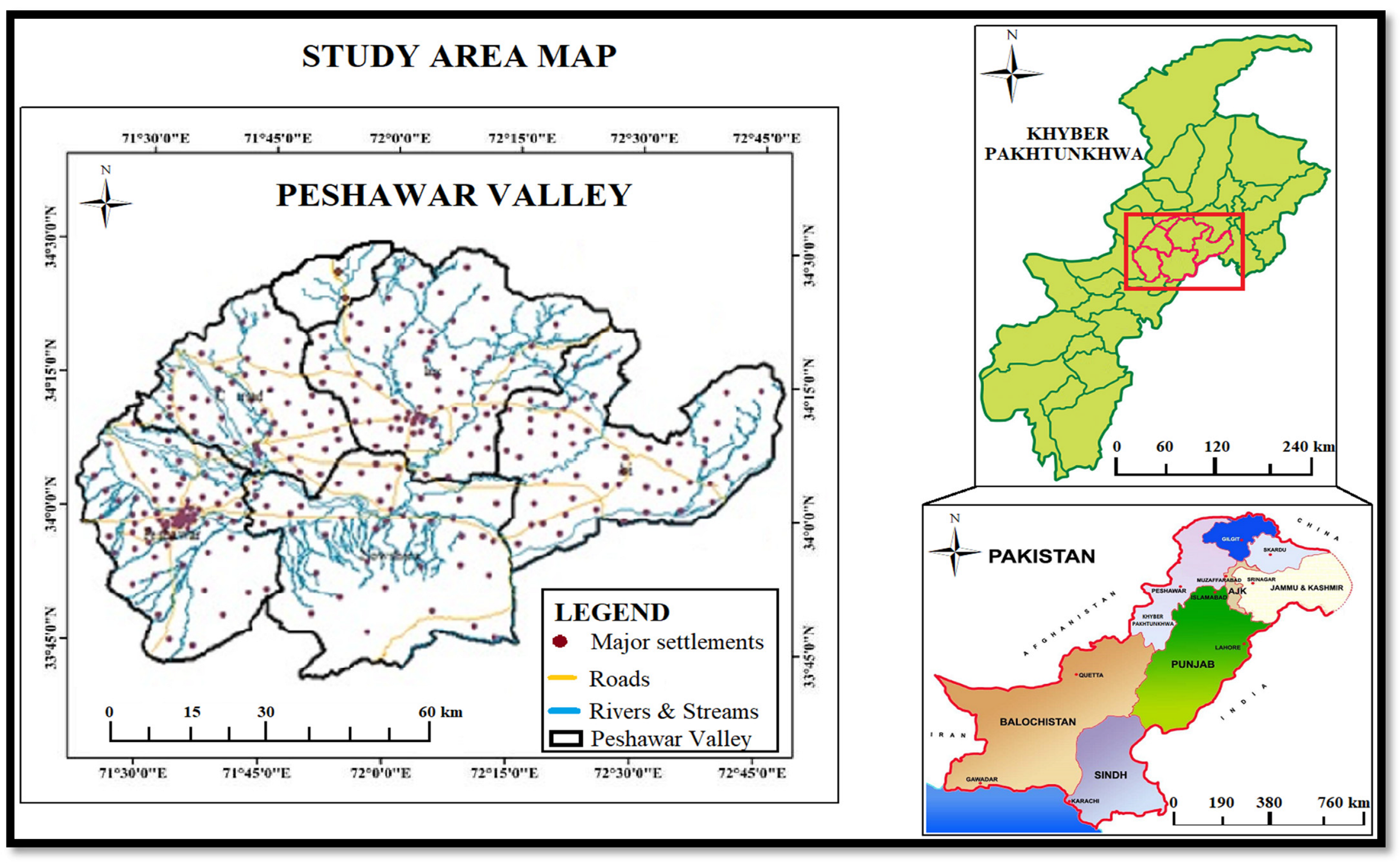
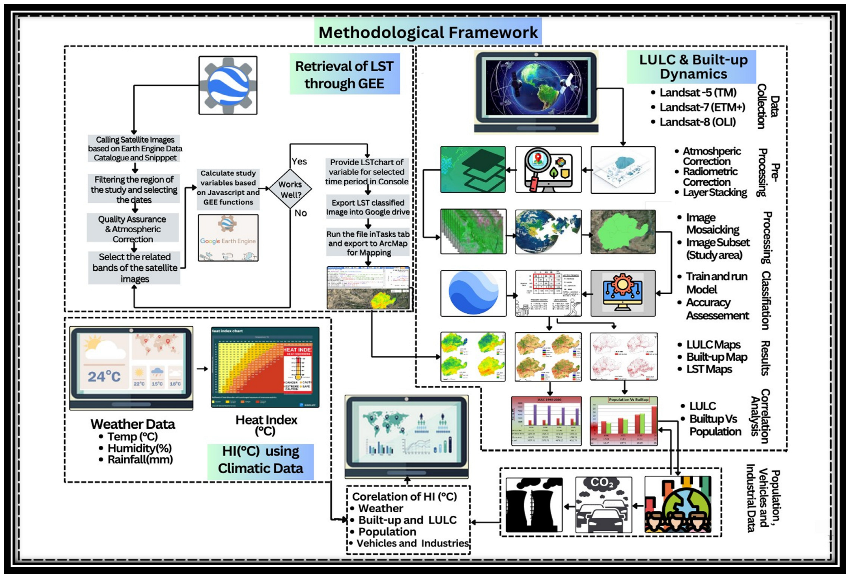
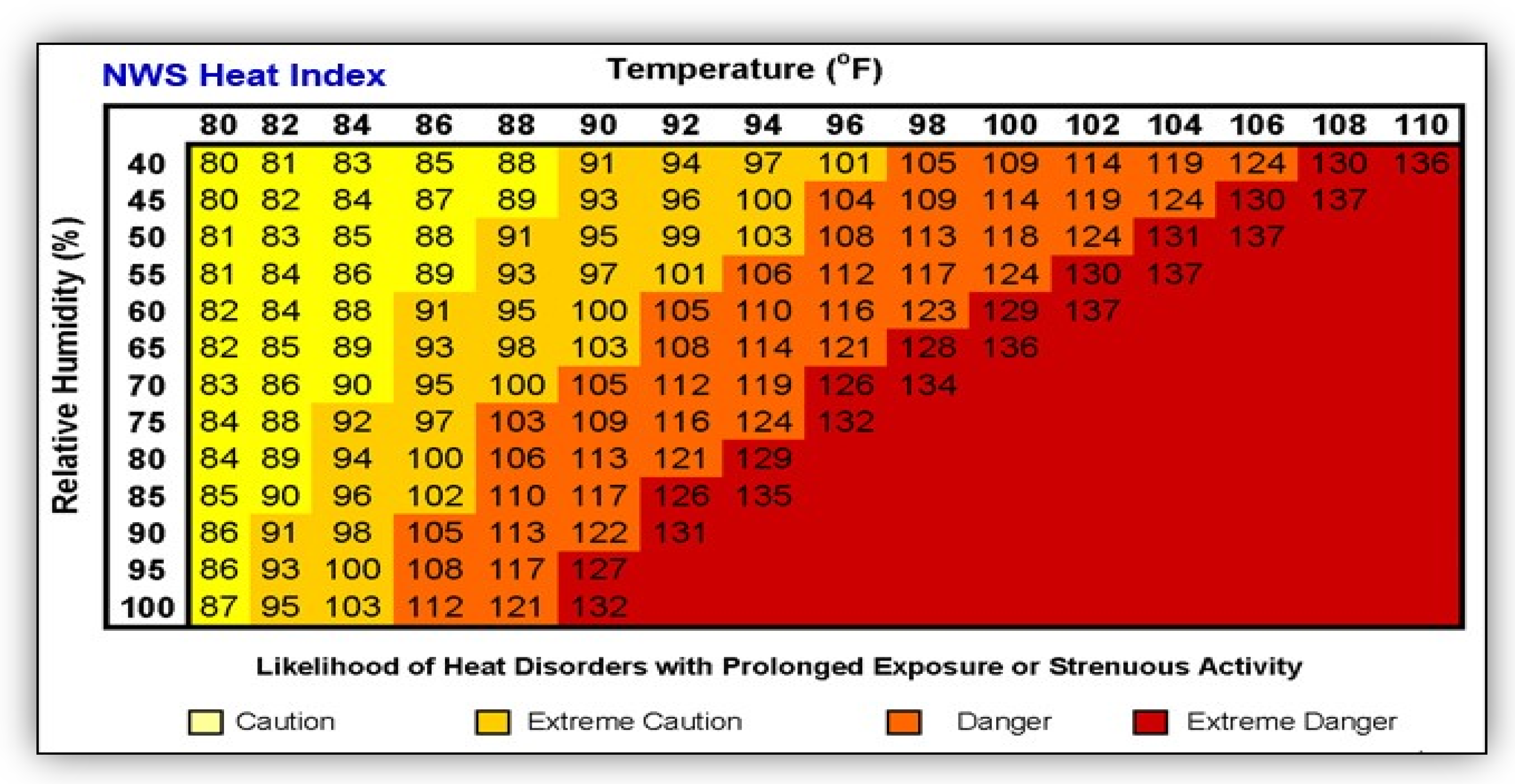
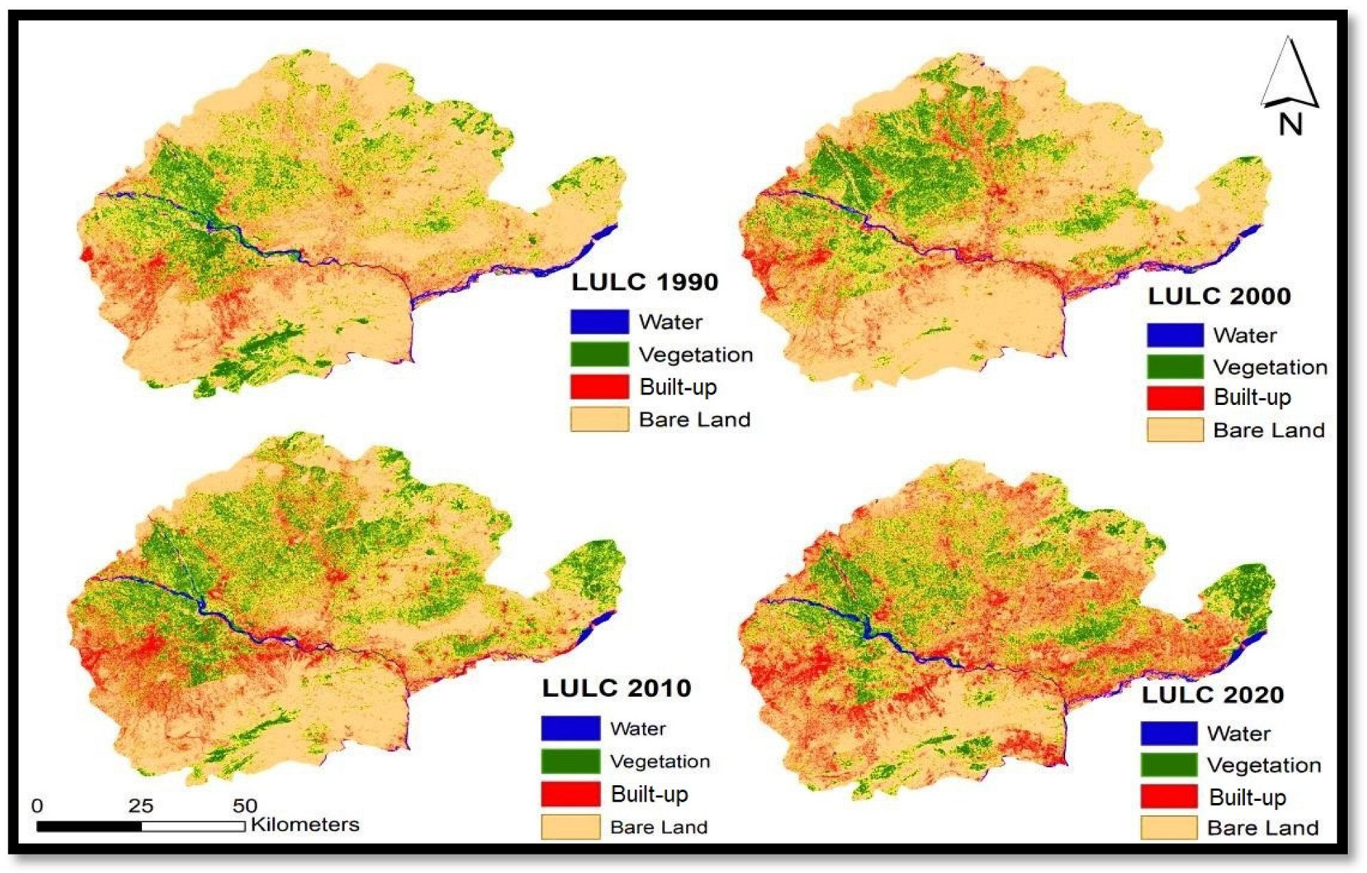
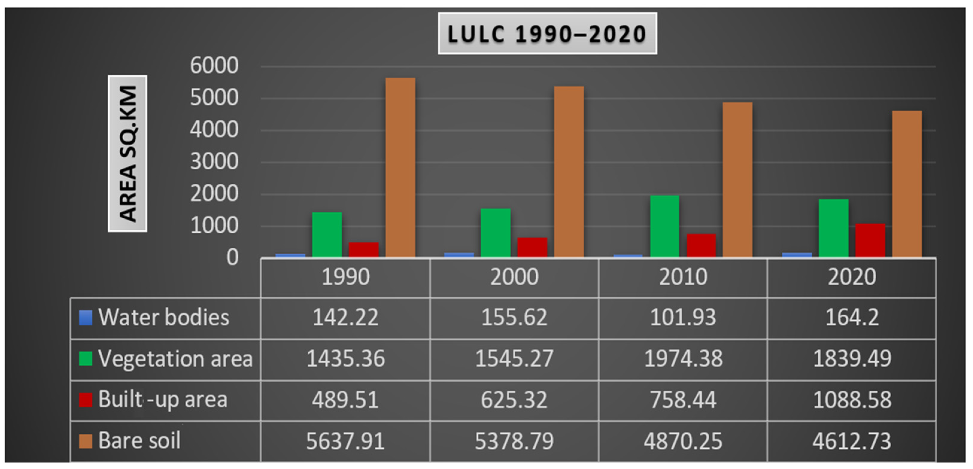

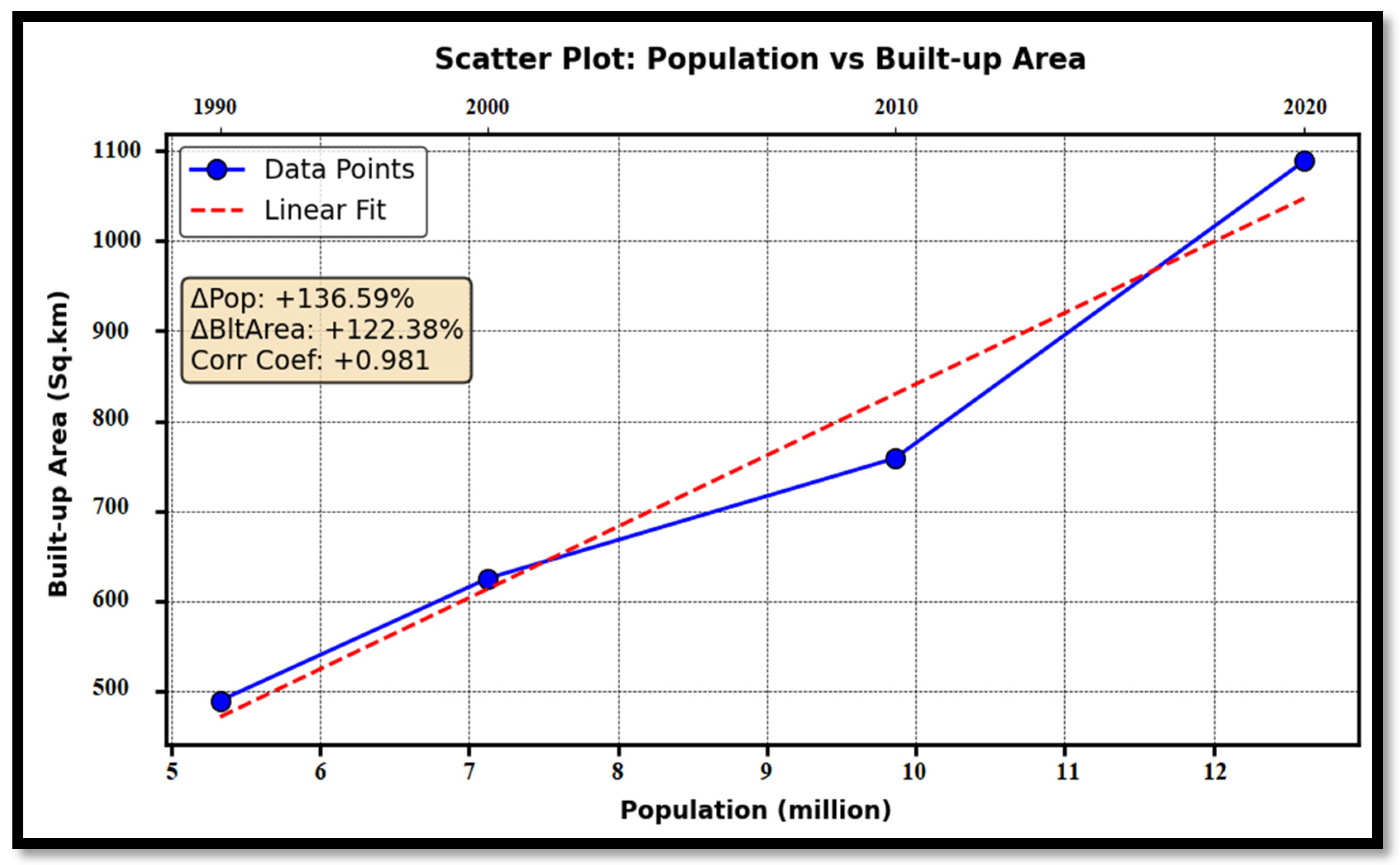
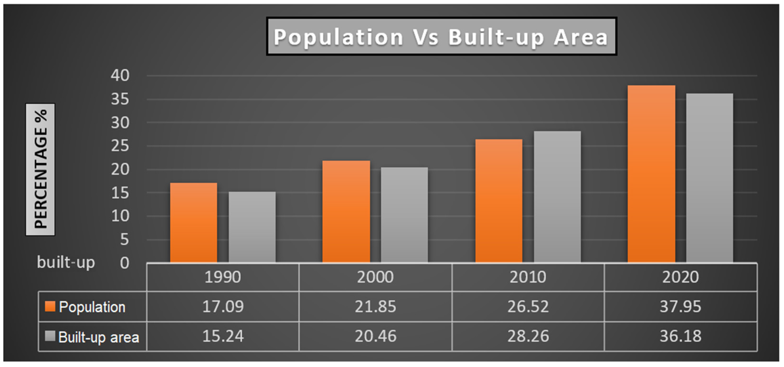
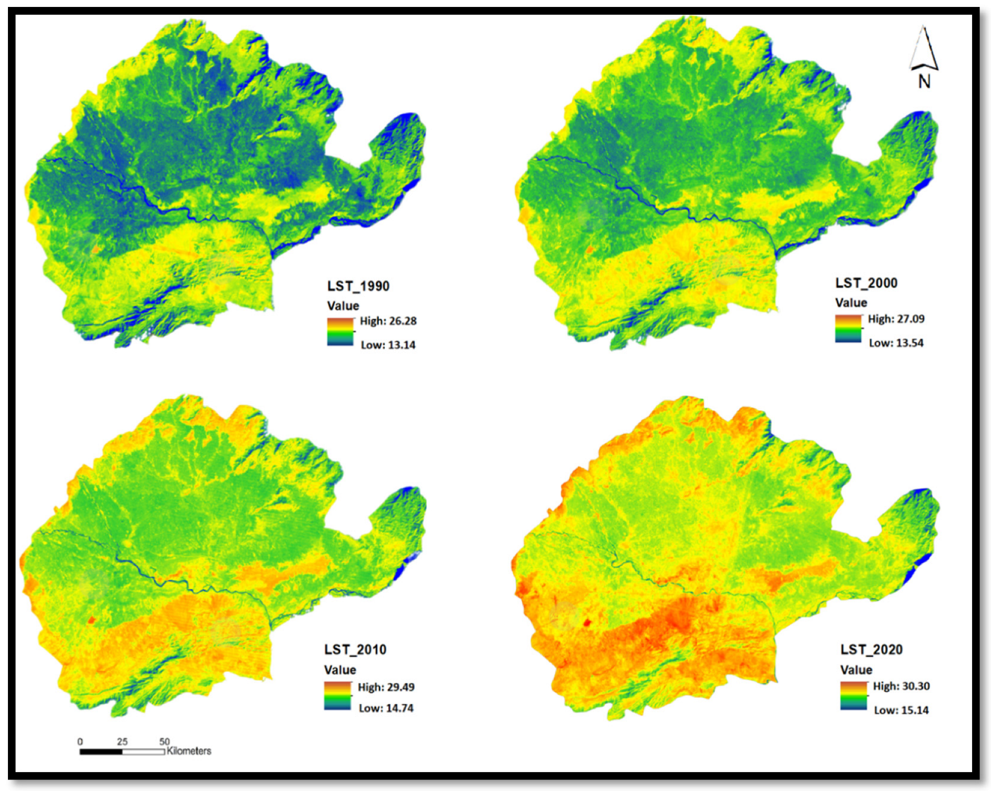
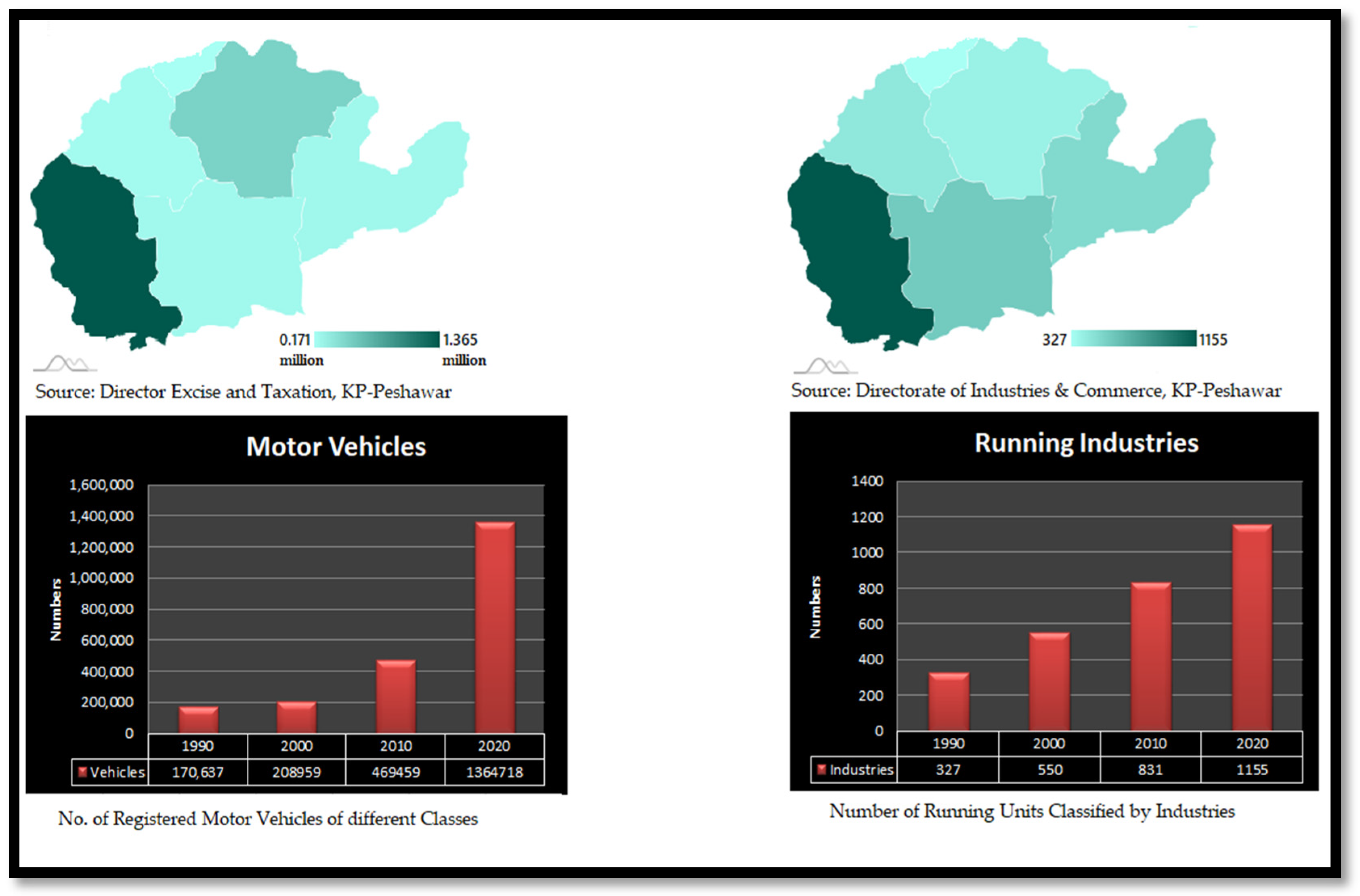
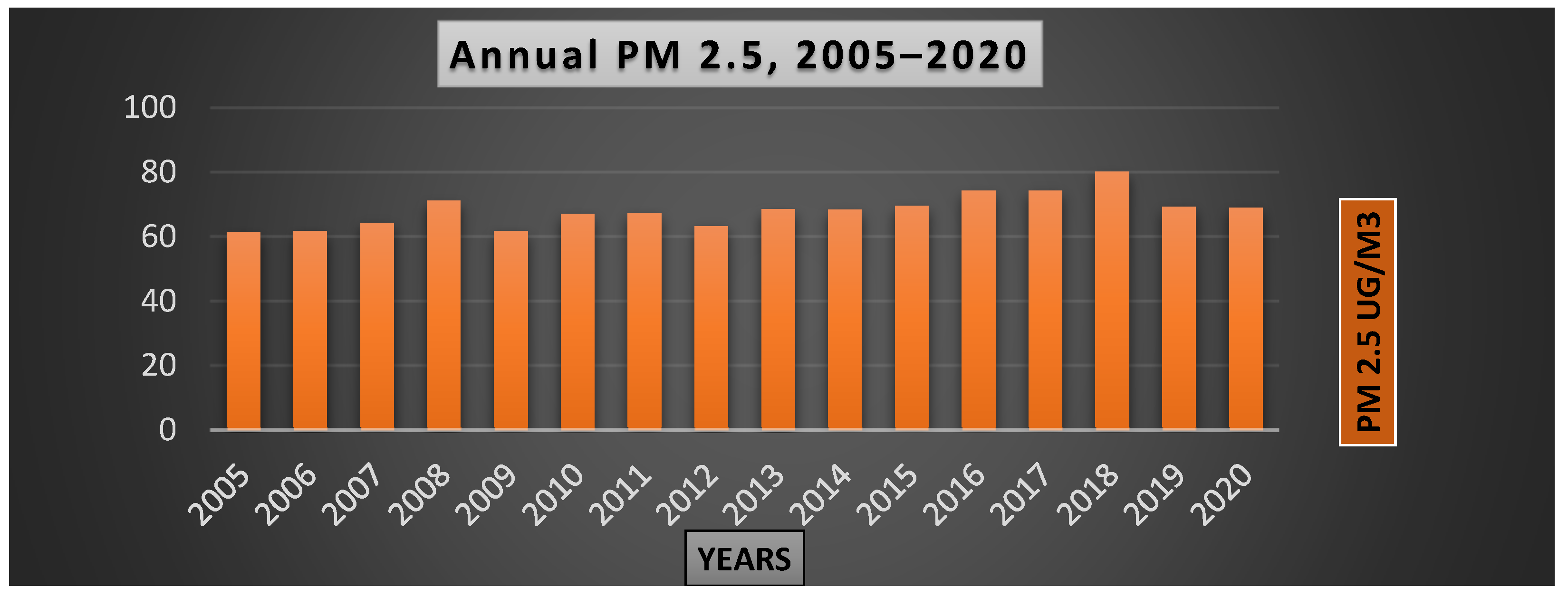
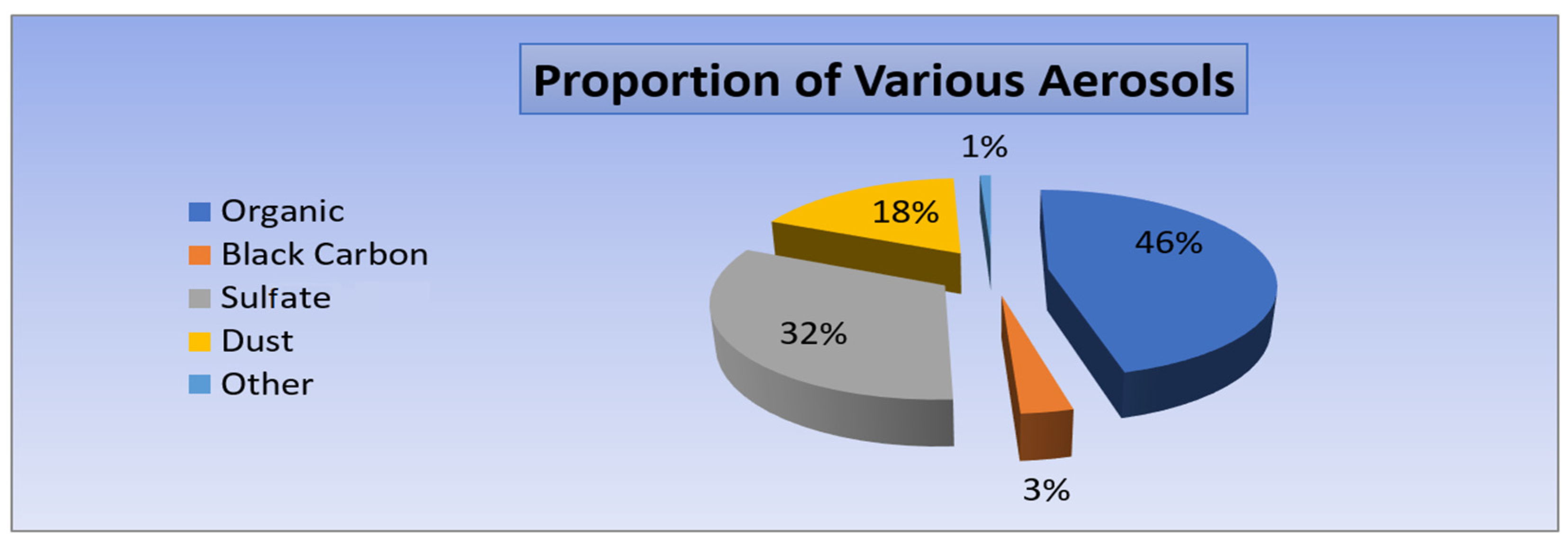
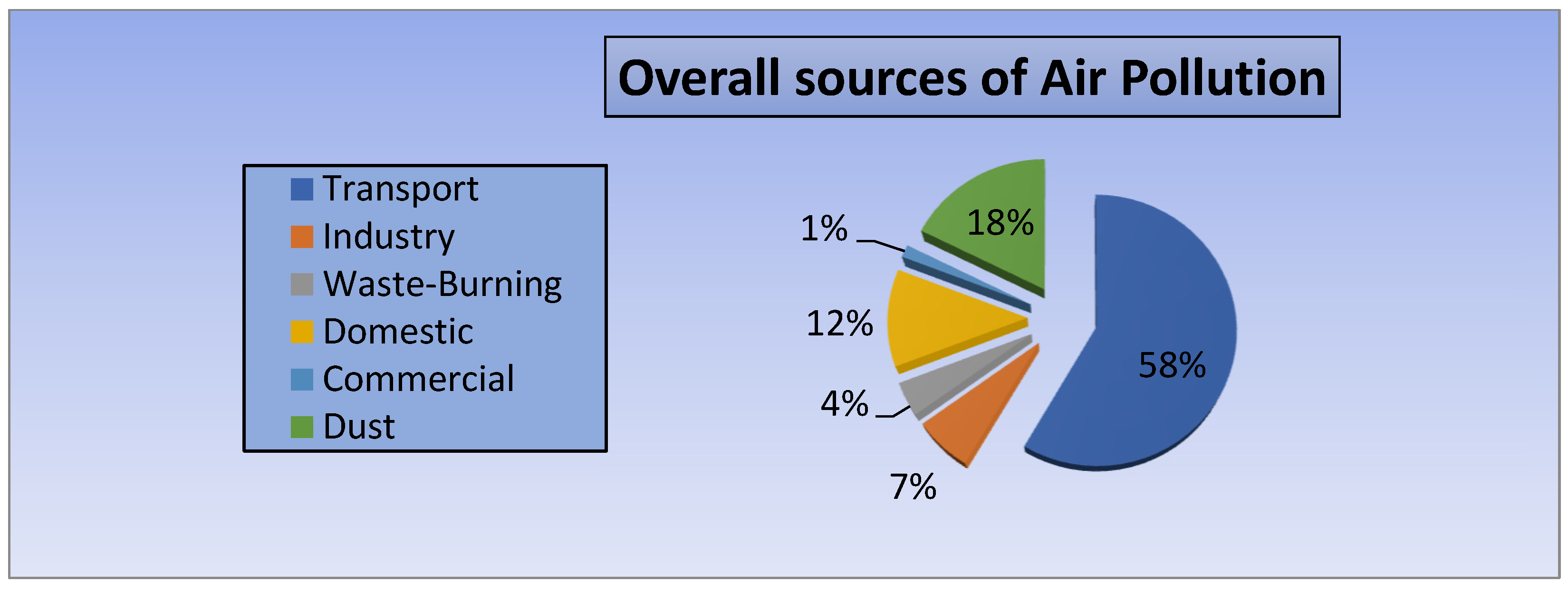
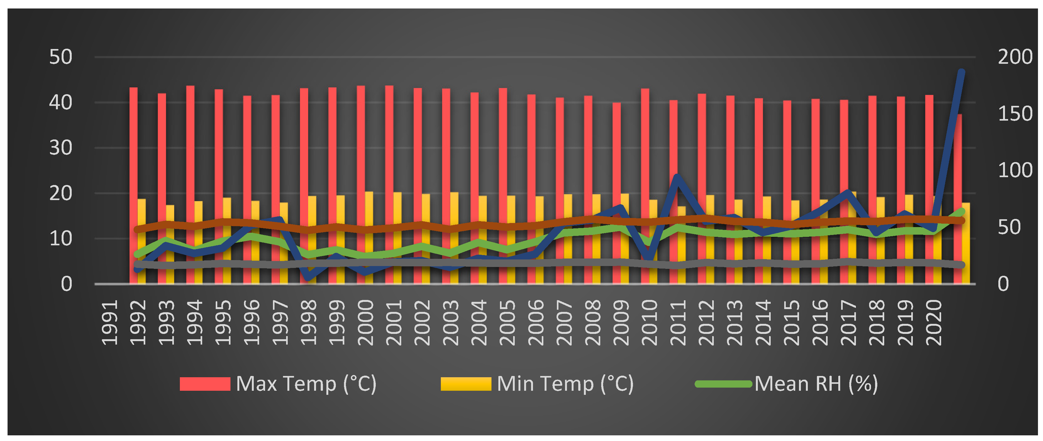

Disclaimer/Publisher’s Note: The statements, opinions and data contained in all publications are solely those of the individual author(s) and contributor(s) and not of MDPI and/or the editor(s). MDPI and/or the editor(s) disclaim responsibility for any injury to people or property resulting from any ideas, methods, instructions or products referred to in the content. |
© 2024 by the authors. Licensee MDPI, Basel, Switzerland. This article is an open access article distributed under the terms and conditions of the Creative Commons Attribution (CC BY) license (https://creativecommons.org/licenses/by/4.0/).