Article

Built Environment Effect on Metro Ridership in Metropolitan Area of Valparaíso, Chile, under Different Influence Area Approaches

by
Vicente Aprigliano
1,*,
Sebastian Seriani
1,
Catalina Toro
1,
Gonzalo Rojas
1,
Mitsuyoshi Fukushi
1,
Marcus Cardoso
2,
Marcelino Aurelio Vieira da Silva
2,
Cristo Cucumides
1,
Ualison Rébula de Oliveira
3,
Cristián Henríquez
4,5,6,
Andreas Braun
7 and
Volker Hochschild
7
1
Escuela de Ingeniería de Construcción y Transporte, Pontificia Universidad Católica de Valparaíso, Avda Brasil 2147, Valparaíso 2362804, Chile
2
Transport Engineering Program, Federal University of Rio de Janeiro, Av. Horácio Macedo 2030, Rio de Janeiro 21941-914, RJ, Brazil
3
Departamento de Administração e Administração Pública de Volta Redonda, Universidade Federal Fluminense (UFF)/MPA-ICHS, MSG-TCE and DSG-TCE, 783 Des. Ellis H. Figueira St Volta Redonda, Rio de Janeiro 27213-145, RJ, Brazil
4
Instituto de Geografía, Facultad de Historia, Geografía y Ciencia Política, Pontifcia Universidad Católica de Chile, Avda. Vicuña Mackenna 4860, Macul, Santiago 8330015, Chile
5
Centro Interdisciplinario de Cambio Global, Pontificia Universidad Católica de Chile, Avda. Vicuña Mackenna 4860, Macul, Santiago 8330015, Chile
6
Centro de Desarrollo Urbano Sustentable (CEDEUS), Pontificia Universidad Católica de Chile, Avda. Vicuña Mackenna 4860, Macul, Santiago 8330015, Chile
7
Department of Geography, University of Tuebingen, Rümelinstr. 19-23, 72070 Tuebingen, Germany
*
Author to whom correspondence should be addressed.
ISPRS Int. J. Geo-Inf. 2024, 13(8), 266; https://doi.org/10.3390/ijgi13080266
Submission received: 24 April 2024 / Revised: 3 July 2024 / Accepted: 23 July 2024 / Published: 26 July 2024

Abstract

:
The growing relevance of promoting a transition of urban mobility toward more sustainable modes of transport is leading to efforts to understand the effects of the built environment on the use of railway systems. In this direction, there are challenges regarding the creation of coherence between the locations of metro stations and their surroundings, which has been explored extensively in the academic community. This process is called Transit-Oriented Development (TOD). Within the context of Latin America, this study seeks to assess the influence of the built environment on the metro ridership in the metropolitan area of Valparaíso, Chile, testing two approaches of influence area definition, one of which is a fixed distance from the stations, and the other is based on the origin and destination survey of the study area. The analysis is based on Ordinary Least Squares regression (OLS) to identify the factors from the built environment, which affects the metro’s ridership. Results show that the models based on the area of influence defined through the use of the origin and destination survey explain the metro ridership better. Moreover, this study reveals that the metro system in Greater Valparaíso was not planned in harmony with urban development. The models demonstrate an inverse effect of the built environment on ridership, contrasting with the expected outcomes of a metro station designed following a Transit-Oriented Development approach.

1. Introduction

The growing relevance of promoting a transition of urban mobility toward more sustainable modes of transport is leading to efforts to understand the effects of the built environment on the use of railway systems. These systems have been gaining significant investments in varied countries, given their potential to significantly reduce the transport sector’s carbon footprint and motorized private transport modes usage [1]. Besides these benefits, Lin et al. [2] add the possibility of transporting people with greater capacity and more efficiently, thus promoting increased urban productivity.
In this direction, there are challenges regarding the creation of coherence between the locations of the transit stations and their surroundings, which has been explored extensively in the academic community [3,4,5,6]; this process is called Transit-Oriented Development (TOD). According to Wey et al. [7], TOD planning is closely related to the transition of cities toward sustainable mobility [7,8], in line with the United Nations’ effort to fulfill the Sustainable Development Goals [9].
The TOD approach appears from the necessity to create functional and lively places around public transport by promoting dense, compact, and walkable spaces [10] in order to generate the benefits highlighted at the beginning of this section. Therefore, it is crucial within the TOD approach to refer to the built environment. According to Cervero et al. [11], the built environment consists of 5 D’s: density, diversity, distance to transit, destination accessibility, and design. Moreover, studies have shown that these dimensions of the 5 D’s may influence people’s choice of transport modes [11,12].
Within the context of Latin America, this study seeks to assess the influence of the built environment on the metro ridership in the metropolitan area of Valparaíso, Chile, testing two approaches of influence area definition. The first of them, based on a radius of 400 m, corresponds to the walkable area as studied by different authors [13,14,15,16,17,18], while the second area proposal corresponds to a population density method that addresses the influence areas through kernel density estimation (KDE) hotspot [19] of walking trip origins of people, which reaches a maximum distance of 250 m from the metro stations, using the data available in the origin and destination survey. The definition of influencing areas of public transport systems, based on people’s actual origin and destination, may deliver a better understanding of modal choice for two reasons. Firstly, because the influence area will be defined based on local particularities regarding mobility behavior and urban characteristics and, secondly, when measuring the impact of these areas on the accessibility and ridership of these modes, results of such analysis may lead to a higher success probability of policies for promoting sustainable mobility.
The latest data show that around 2% of trips in the Metropolitan Area of Valparaíso (also known as Greater Valparaíso) are made by metro, 27% by bus, 29% private transport, and 27% by non-motorized modes [20]. On the other hand, the State Railway Company of Valparaíso (Also known as EFE Valparaíso) has been implementing measures to increase the capacity of the service [21] by increasing frequency in the peak hours. However, this study seeks to understand the external factors of the metro stations that possibly are generating influence on metro ridership and which, usually, are not taken into account by transport planners in Greater Valparaíso.
According to Aprigliano et al. [22], there is a need to advance mobility studies, which are applied to small and intermediate cities. The authors state that most studies within the Latin American context are focused on large cities. In Chile, this is not different; most mobility and transport studies are dedicated to Santiago and Concepción, both having the largest metropolitan areas in this country. Regarding Valparaíso, it is the third-largest metropolitan area in Chile, with approximately 1 million inhabitants, and composed of five cities: Villa Alemana, Quilpué, Concon, Viña del Mar, and Valparaíso. Respectively, they have 126,548 (13% of the population of Greater Valparaíso), 151,708 (16%), 42,152 (4%), 334,248 (35%), and 296,655 (31%) inhabitants. The metro system comprises one line with 43 km and 20 stations. Furthermore, four of the cities in the study area have metro stations, which can be observed in Figure 1.
It is important to note that the current public transport systems in Greater Valparaíso compete with each other in many cases, instead of having a synergy between feeder and main public transport lines (see Figure 1). In addition to this, there is a slow process of updating land use regulations in the cities of Greater Valparaíso [23], which are called “planes reguladores comunales”. This instrument is relevant for urban development because it can be a barrier or an instrument that effectively leads to urban sustainability for Chilean cities [24].
These previously mentioned conditions can influence the promotion of sustainable mobility in Greater Valparaíso, given an incoherent relation between transport and land use development. In the case of the metro system in Greater Valparaíso, there is an expansion plan for the metro line [25]. A lack of understanding of the metro station’s surrounding influence area in relation to its ridership can lead to issues with the station’s attractiveness. Additionally, failing to leverage a system that could enhance urban productivity and accessibility through Transit-Oriented Development (TOD) planning represents a missed opportunity. This study is a contribution to studies related to intermediate cities and can shed some light on how to advance toward more sustainable intermediate cities in Chile and Latin America through efficient and attractive public transport systems.
Besides this introduction, the literature review section is dedicated to reviewing case studies that relate to the built environment and metro ridership in a determined influence area. Then, there is the methodology section, which focuses on describing the case study, variables, and methods. The results section analyzes and interprets the outputs of the applied methods. Finally, the conclusion and final considerations section provides a general perspective of the results, limitations of the study, and future research opportunities.

2. Transit’s Influence Area and Metro Ridership: A Review

In this paper, the concept of the influence area of a given metro station is understood as the catchment zone for both current users and potential users of the system. According to Taylor & Fink [26], a multitude of factors impacts the usage of public transportation, encompassing fares, routes, service frequency, accessibility of stops and stations, safety, levels of private vehicle ownership, population density, land use and its availability, parking cost, among various other considerations.
Different factors may contribute to the reduction in the number of passengers in transit, such as increased car and bicycle ownership or even the lack of reliability in transit services [27]. Many studies also associate travel behavior with weather factors [28,29,30,31] and, therefore, would be directly linked to transit ridership. Furthermore, other studies indicate that socioeconomic factors such as car ownership, income, gender, and age are also associated with individuals’ choices regarding the use of public transportation [32,33]. Besides external factors beyond human control, transit ridership is also affected by a broad spectrum of human factors, which can typically be classified into three groups: individual-level, station-level, and system-level factors [34].
Generally, TOD entails establishing zones with moderate to high density that feature a mix of land uses within a convenient walking distance, typically around 800 m, from public transportation stations [35]. This section seeks to undertake a literature review of how studies have been defining the influence area of metro stations and the factors influencing their ridership, focused on non-motorized accessibility to these stations. On the other hand, according to Sohn & Shim [36], in the metropolitan area of Seoul (Republic of Korea), the catchment area of metro stations, considering pedestrian access by passengers, was investigated, and a radius of 500 m was accepted as the standard for transportation studies.
Ramos-Santiago [37] conducted a study in the city of Los Angeles, aiming to investigate the local multimodal transit network to explore whether the walkability quality around feeder bus line stations could affect the number of station ridership at the metro system. The study employed a multilevel generalized linear model using data on pedestrian accessibility at bus stops, along with relevant variables, to identify the volume of trips between feeder bus lines and metro stations and their potential correlation with land use and built environment characteristics around feeder bus line stations. The findings indicated a weak but statistically significant influence between the walkability quality around feeder bus line stations and the number of passengers boarding at metro stations.
In order to explore the relationship between various independent variables and urban rapid transit ridership at the station level and identify the influence of spatial heterogeneity in a subway network in the city of Nanjing, China, Gan et al. [38] estimated four statistical models separately. Initially, based on data from the built environment and station characteristics, the results show evidence of the existence of spatial heterogeneity in station usage for the analyzed subway network. Furthermore, the results demonstrate that population, number of lines, number of feeder buses, number of exits, road density, and proportion of residential area have a significant impact on station ridership.
With the aim of evaluating the land use characteristics around metro stations in the Seoul metropolitan region (South Korea) and their influence on pedestrian catchment areas, in terms of principles of TOD, Jun et al. [39] found that population and employment density, land use diversity, as well as intermodal connectivity, have a positive impact on subway usage. The study also demonstrated that, in Seoul, the most suitable catchment radius for a metro station is 600 m.
In a study conducted in Beijing, China, using the metro system as a case study, Zhao & Li [40] identified that travel distances between home and transit stations are the most important factor influencing people’s decisions to cycle or not.
To explore the relationship between public transportation ridership demand and TOD indicators, Nyunt & Wongchavalidkul [41] conducted a study analyzing variables collected within an 800-m buffer around public transportation stations, using the Bangkok metro system in Thailand as a case study. The results revealed that high population density, mixed land use, and the function of a station as a transfer point between different modes and systems of transportation are some of the key factors impacting the catchment area and, consequently, influencing the attractiveness of a particular metro station to users.
He et al. [42] investigated in Shenzhen, China, using a geographically weighted regression-based direct demand model, the local relationships between passenger demand at metro stations, and potential influencing factors. The influencing factors considered included land use, local socioeconomic characteristics, transport network structure, and access to intermodal transportation. The research indicates that there is a positive correlation between betweenness centrality and station ridership volume, suggesting that the significance of a station in facilitating the shortest routes within the metro network plays a crucial role in attracting additional passengers.
In the study conducted by Gupta et al. [43], the impacts of various subjective and objective factors of the built environment on users’ decisions regarding access mode to metro stations were investigated. Through interviews with 600 metro users in the city of Delhi, India, socioeconomic information and details about travel characteristics were collected. The study’s findings revealed that neighborhood built environment characteristics, along with population density and land use, play a significant and positive role in the choice of metro transportation. Furthermore, it is suggested that improvements in the built environment attributes within the catchment areas of metro stations will lead to an increase in the proportion of users opting to access them on foot.
By utilizing large-scale data and non-parametric machine learning approaches, Liu et al. [44] conducted a study in the city of Shanghai, China, aimed at conducting a sensitivity analysis to examine the association between metro usage and built environment factors within different sizes of radial buffers. As a result, the study suggests that a buffer size of 600 m around the metro station provides the best fit for the predictive model of station access.
Based on a modeling approach to explore the impact of land use, metro service coverage, and station accessibility on metro ridership in six cities in the United States, Li et al. [45] concluded that the optimal radius of the metro passenger capture buffer is not the same across different cities. The study also demonstrated that the number of automobile owners, the urban population, the number of workers, and income have a significantly positive influence on the number of metro passengers.
The present study addresses two types of influence areas of metro stations, seeking to compare built environment aspects and their effect on metro ridership. Additionally, this research complements the literature presented by exploring an influence area determined by origin and destination survey data and a fixed influence area, which avoids overlapping between stations. Furthermore, considering that the case study combines different intermediate cities in a metropolitan area of Chile that lacks studies that relate to the built environment and mobility patterns, the results may shed light on future planning of cities in Latin America with similar demographic and urban dimensions.

3. Materials and Methods

To meet the proposed objectives, a methodology was developed that included 5 stages, which consisted of the following:
  • Collection of secondary information: information was obtained from the origin and destination survey [20], Chile’s railway network [46], traffic accidents [47], and creation of the vector layer of the subway stations.
  • Creation of surrounding influence areas of metro stations.
Areas of influence were defined in the surroundings of the metro stations in two ways, which are detailed below.
Firstly, influence areas were generated in QGIS through a 400 m radius buffer for each station, resulting in 19 influence areas. Then, a cut was made to those areas of coastal stations that exceeded the territorial limits and covered areas of the sea to obtain only the area covered on dry land. Furthermore, this area was defined to avoid overlapping of influence areas between stations.
Secondly, other areas were obtained from the spatial identification of people who go to an area with a radius of 250 m from the metro stations, identified from a pair of coordinates available in the origin and destination survey, obtaining the peoples’ points of origin and destination. A kernel density estimation (KDE) was applied to peoples’ points to define a new influence area. This method has been used to detect and analyze hotspots [19] of events that can be represented as points, such as traffic accidents, street crimes, and crime areas, among others [48]. This identification was achieved using the destination coordinates of people and then obtaining the origin coordinates of those people, grouping them by station. From the above, points were obtained from people who live and go to areas within a 250-m radius of the stations. Once the points were identified, a kernel density estimation (KDE) was carried out in those areas that have 5 or more points of origin, which results in a raster with densities based on these points. Subsequently, the raster was reclassified based on a selection of a pixel that was at the ends of the densest areas and thus generating two classes, those pixels that are greater or less than the selected pixel, that is, outside or within the densest area (See Table 1). These pixel values represent the density of people in an area in square meters (m2) and are small because the sample used to generate the KDE was small, so it represented few people. In this case, the area is 100 square meters because the pixel is 10 m.
Depending on the number of points, there may be several results of dense areas, so the area closest to the corresponding station was selected. Finally, a vectorization of the reclassified raster was carried out to finally eliminate those polygons far from the corresponding station and leave the closest and most representative one, which represents the area of influence of the station, resulting in 9 areas of influence (see Table 2).

3.1. Urban Environment Indicators in the Area Surrounding Metro Stations

To understand the characteristics of the stations’ built environment in their influence area, urban environment indicators were generated based on the 5 dimensions proposed by Cervero et al. [11], which are density, design, destination, distance, and diversity. Besides the explanation below, Table 3 presents details about the indicators and source of information.
The “density” dimension consists of a proportion between the total number of households and the area of each influence zone. To obtain this indicator, the census block was used, whose area in hectares was calculated, to subsequently cut it by the area of influence of each station and recalculate the area of the blocks within the areas of influence. This is in line with the objective of generating a proportion that allows for obtaining the number of homes within the defined blocks in relation to the homes in the original blocks. To perform this, a multiplication was generated between the area of the cut blocks and the total number of homes and then divided by the area of the complete block. Finally, the number of households within each area of influence was added, the result being divided by the area of influence of each metro station.
The second dimension, “design”, contains two variables—street design and safety—which consist of the number of nodes per number of streets in topological terms and the number of accidents per hectare, respectively. The first variable (street design) was generated in Python, using the geopandas and pandas libraries, where the Red Vial vector layer [46] was used. It was cut to the surrounding area of each station to generate points or nodes of the intersections of each street and finally, count and then divide the number of nodes by the number of streets.
On the other hand, for the safety design variable, the vector layers of traffic accidents for the years 2018, 2019, 2020, and 2021 available in CONASET [47] were used for the metropolitan area of Valparaíso. Using the geopandas and Python pandas libraries, the accidents were filtered by those accidents identified as “Falls” and/or “Runovers”, that is, accidents related to pedestrians. Subsequently, the result of this filter was cut to the area surrounding the metro stations, obtaining a certain number of accidents within each area. Finally, all the accidents present in each area were averaged and added (that is, accidents for the years 2018, 2019, 2020, and 2021), and the resulting total was divided into the hectares of each surrounding area of influence.
For the “destination” variable, the walking score provided by Walkscore was used, which considers various services close to or non-existent from the address given, such as restaurants, bars, supermarkets, commercial premises, services, parks, schools, and places of culture and leisure [49]. Access to these scores was made through the Nominatim [50] and Walkscore (free version) APIs using the Python libraries pandas, geopandas, requests, json, and urllib.parse, along with the calculated areas. The process was based on extracting the centroid of each area in QGIS 3.28, storing a pair of coordinates for each area. These coordinates were used in the Nominatim API (respecting the limits of use), and the resulting addresses were used in the WalkScore API (free version) in Python to obtain the walk score of each area.
Fourth, the “distance” dimension was obtained from a Google Maps search of the route from each station to its nearest bus stop. Finally, the “diversity” dimension consists of identifying the proportion of residential land use in the different areas of influence of the metro stations. To obtain this indicator, the Municipal Regulatory Plan (known as PRC in Chile) of Valparaíso, Viña del Mar, Quilpué, and Villa Alemana was used [51]. The objective was to identify the proportion of residential use over other permitted land uses. The PRCs, provided in shapefile format, were processed in QGIS 3.28, where they were cropped to coincide with the influence areas of the metro stations. Within each area of influence, the residential areas (including residences, homes, hotels, etc.) were identified and filtered, and the total residential area in hectares for each area of influence was calculated. Finally, this surface was divided by the sum of all permitted areas (other uses) in the area of influence of each metro station. See Table A1 in the Appendix A for more information on how each indicator was calculated.
Table 3. Urban environment indicators with which the models will be executed. Source: elaborated by authors.
Category Dimension IndicatorsDescriptionSource DataReferences
Urban environment Density Housing Dwelling units per total area, expressed in hectares (Ha)Block Census of Gran Valparaíso [52]Cervero et al., 2009 [11]
Design Street design Number of Nodes per Number of topological Streets Street network: polylines of streets in Chile [46]Cervero et al., 2009 [11];
Motieyan & Mesgari, 2017 [53]
Street safety: Number of vehicular accidents per area expressed in hectares (Ha) Traffic accidents, Valparaiso Region, Chile, 2018–2023 [47]Cervero et al., 2009 [11];
Motieyan & Mesgari, 2017 [53]
Destination WalkScore Find the centroid of each zone and enter the addresses into Walkscore.com (accessed on 17 January 2024), which calculates this score for each zone up to 0.6 miles away.WalkScore API (free version) [49] and APIs Nominatim [50]Cervero et al., 2009 [11];
Zhang et al., 2023 [54]
Distance Distance to the nearest bus stop The distance from the train station to the nearest bus stop Google Maps [55]Cervero et al., 2009 [11];
Zhang et al., 2019 [56]
Diversity Mixed land Use: The ratio of the residential area to total area expressed in hectares (Ha).PRC from the municipalities of Valparaíso, Viña del Mar, Quilpué, and Villa Alemana [51]Cervero et al., 2009 [11];
Pongprasert & Kubota, 2018 [57]

3.2. Regression Models Applied

Ordinary Least Squares (OLS) regression models are employed to analyze the factors influencing ridership levels at metro stations. The model evaluates the relationship between passenger flows and various attributes of the built environment surrounding the stations. The selection of OLS regression is motivated by its capacity to handle both numerical and categorical data types. The approach follows the precedent set by previous research that highlights the model’s effectiveness in this field [58,59,60].
To conduct this analysis, the dependent variable is defined as the average passenger boarding flow at each metro station. The independent variables encompass aspects of the built environment, such as “density”, represented by the ratio of dwellings to the area of each station’s influence zone; “design”, which includes urban design elements like street layout and safety metrics (e.g., accident rates per hectare); “destination”, gauged by a walkability index that reflects accessibility to essential services; “distance”, measured as the proximity to the nearest bus stop; and “diversity”, which assesses the variety of land use within the station’s influence zones. This array of variables provides a comprehensive framework for exploring how environmental factors impact metro ridership. In addition, the effect of seasonal variation in the flows is modeled using a categorical variable that differentiates by seasonality into holiday and regular seasons.
The estimation of the OLS regression models was carried out using data collected from two distinct methodologies to determine the areas of influence around metro stations. The first method involved 19 stations, while the second method considered 9 stations. Each method aimed to capture unique variations in spatial distribution and environmental impacts on ridership levels. The timeframe for the study spanned from 2018 to 2023, and a model was estimated for each year. The models that demonstrated the best performance in terms of explanatory power are highlighted and analyzed in the subsequent sections. This approach aims to provide an understanding of the built environment’s role in shaping metro station ridership.

4. Description of Case Study

This study focuses on the Metropolitan Area of Valparaíso (Also known as Greater or Gran Valparaíso), specifically on the EFE Valparaíso metro network present in this area, which covers the cities of Valparaíso, Viña del Mar, Concón, Quilpué, and Villa Alemana, with a population of 951,311 inhabitants [61]. In terms of population, it is relevant to highlight that there are slightly higher numbers of women than men in these cities. Furthermore, Viña del Mar is the most populated municipality, with 334,248 inhabitants, while Concón registers the smallest population, with 42,152 inhabitants, as detailed in Table 4.
The EFE Valparaíso network extends along 43 km of double electrified railway track, connecting a total of 20 stations in the cities of Valparaíso, Viña del Mar, Quilpué, Villa Alemana, and Limache [62]. However, the municipality of Limache is located outside Greater Valparaíso, so for this study, it was considered up to the Peñablanca station, which is the last station of Villa Alemana (Figure 2). In relation to the aforementioned, the distance between the first station (Puerto, Valparaíso) and the last station within Greater Valparaíso (Peñablanca, Villa Alemana) is approximately 30 km. Of the 20 stations, 16 are at surface level, and four are located underground: Hospital, Viña del Mar, Miramar, and Chorrillos, all in the city of Viña del Mar [62].

4.1. Socioeconomic Aspects for Municipalities of Greater Valparaiso

Regarding the sociodemographic characteristics of the municipalities in the Greater Valparaiso area covered by the subway network, there are differences between the characteristics. Firstly, in terms of the total population, Viña del Mar leads with 389,059 inhabitants, followed by Valparaiso with 306,236, Quilpué with 174,203, and Villa Alemana with 126,583. The proportion of the female population regarding the total population does not show major differences, with Villa Alemana having the highest proportion of women with 0.51. As for the average age, there are no major differences, ranging from 35 to 37 years old, with Viña del Mar being the oldest at 36.27 and Villa Alemana the youngest at 35.73.
In terms of socioeconomic characteristics, household size is larger in Villa Alemana but not much larger than in the rest of the municipalities, being between 2 and 3 persons per house. Car ownership per household is most common in Viña del Mar, with 0.66 cars per household. Household income is highest in Viña del Mar, with an average of 878,705 pesos Chilenos (Chilean currency), followed by Valparaiso, Quilpué, and Villa Alemana. These data provide a detailed view of the distinctive demographic and socioeconomic characteristics of these Chilean cities (see Table 5). See Table A2 in the Appendix A for more information on how each characteristic was calculated.

4.2. Concentration of Trips in Areas of Influence of 250, 500 and 750 m

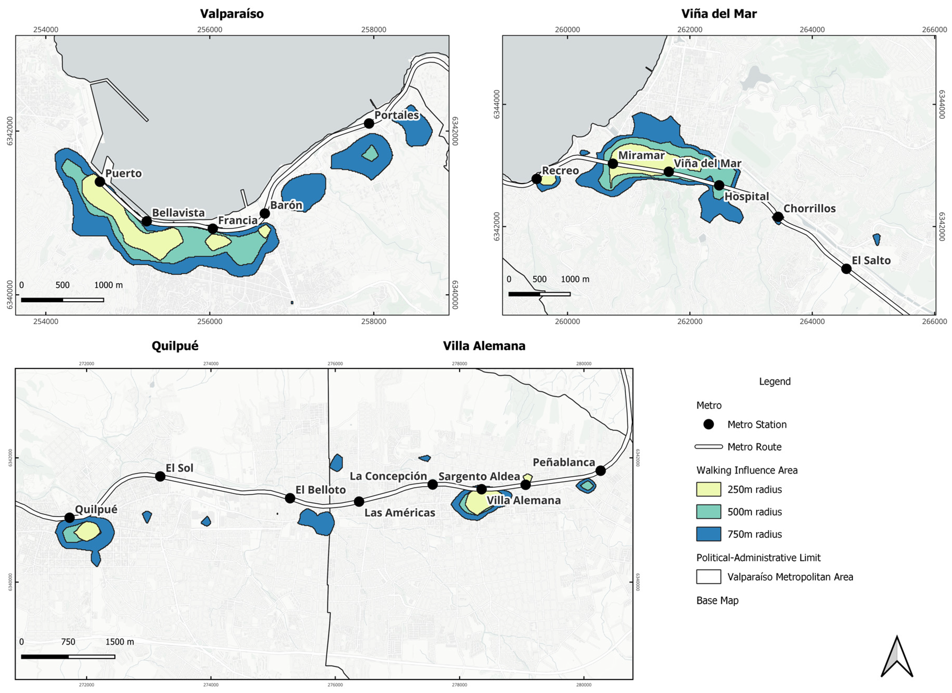
Based on the information from the origin and destination survey [20], we obtained the origin and destination coordinates of people going to the areas of influence of the metro stations previously calculated from buffers of 250 m, 500 m, and 750 m. Once the origin points of people going to these areas were identified, a kernel density estimation was performed for the three areas. Then, the area was selected through a manual identification of denser pixels to reclassify and finally vectorize the area to obtain the areas shown in Figure 3.
According to this information, there is a prominent concentration area for metro stations in the commune of Valparaíso between Puerto and Bellavista. On the other hand, there are isolated areas for Francia and a more distant and smaller area around Barón station. As the radius of influence is extended to 500 m, a continuous zone can be seen between Puerto and Francia. In the area of influence of 750 m, the concentration between the Puerto and Barón stations expands even further, generating areas near Barón and Portales.
In the case of Viña del Mar, there is a main concentration between the Miramar and Viña del Mar stations, which expands as the radius of influence increases, reaching the Hospital stations in an area of 500 and 750 m. The Recreo station presents a smaller and more isolated area, while Chorrillos and El Salto show very small and isolated concentration areas.
For the network in Quilpué and Villa Alemana, two main concentration areas are identified near the Quilpué and Villa Alemana stations, which increase in size with each radius of influence.

4.3. Concentration of Trip by Mode of Transport

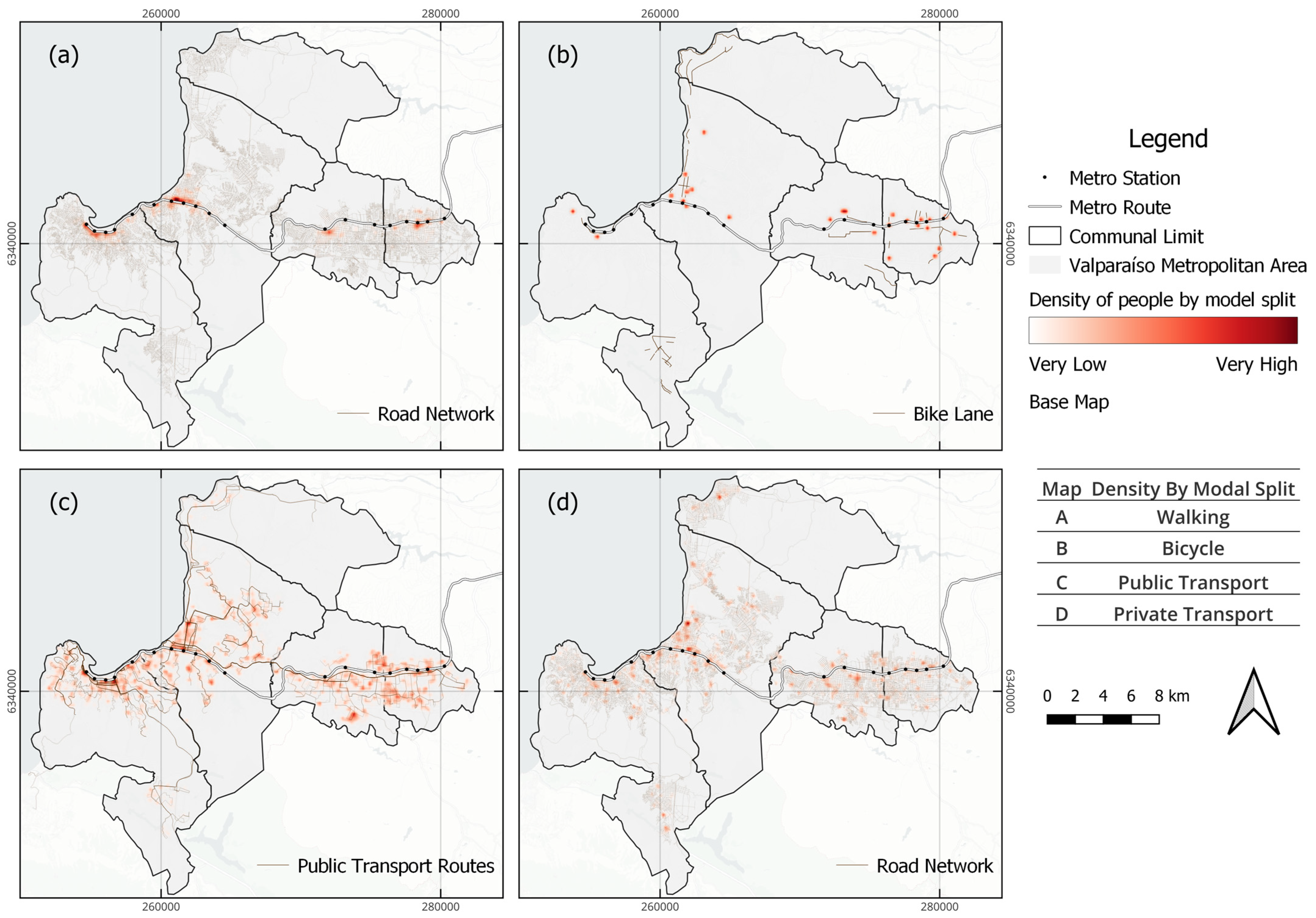
The concentration of the origin of people who go toward an area of influence of 250 m around the metro stations shows that public transport (Figure 4c) has the greatest coverage in the Metropolitan Area of Valparaíso. This is followed by a slightly more dispersed concentration of private transportation (Figure 4d), while walking is observed more punctually in the vicinity of the metro stations, with a greater concentration in Valparaíso and Viña del Mar (Figure 4a). Regarding the origin of those who go to the area of influence of the metro by bicycle, it is much more individualized and does not generate significant concentrations (Figure 4b).
This analysis was possible thanks to the data provided by the origin and destination survey [20] since it contains the georeferenced identification of the start and end point of the trip of each person interviewed, as well as the modal split used to travel. From this information, a kernel density estimate was generated with the points of origin of each person by modal split.

4.4. Passenger Flow between Puerto and Peñablanca Stations (2018–2023)

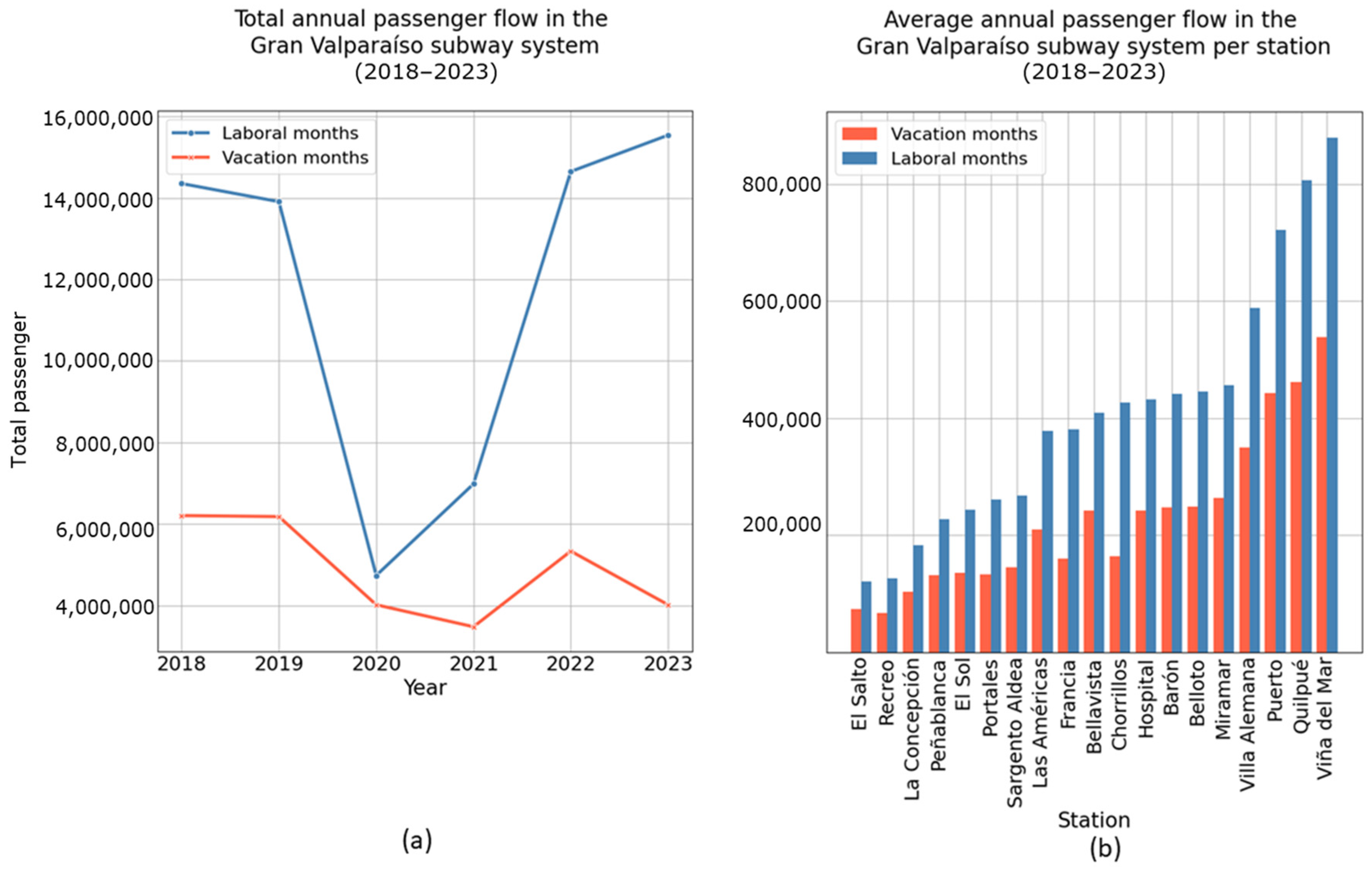
In the section of the Valparaíso metro between the Puerto and Peñablanca stations, the upward flow of passengers averaged 10,163,094 trips between 2018 and 2019. However, this number fell to an average of 4,802,914 trips in 2020 and 2021, which represents a decrease of 52.7%, mainly attributed to the restrictions imposed by the SARS-CoV-2 health crisis. In the period from 2022 to 2023, a recovery was observed with 9,885,774 trips, which is equivalent to an increase of 105.8% compared to 2020–2021 and only 2.7% less than in 2018–2019, according to data provided by EFE [63].
To facilitate the flow analysis, the sample was divided into work months (March, April, May, June, August, September, October, and November) and vacation months (January, February, July, and December), guided mainly by the student calendar. Regarding the distribution of trips in the mentioned periods, similar trends are maintained in both seasons, as seen in Figure 5a.
Regarding the average number of passengers per station and season, consistent behavior is evident between stations and seasons, with a lower flow of passengers during the vacation period. Viña del Mar, Quilpué, and Puerto are the stations that present the highest flow for both the vacation period and the work period, exceeding 400,000 boarding trips for the vacation period and exceeding 721,760 boarding trips for the work period, particularly the Viña del Mar station, reached 879,883 in work months and 537,873 in vacation months. On the other hand, El Salto and Recreo present the lowest flows, with less than 70,000 for the vacation period and 130,000 trips for the work period.
Furthermore, a marked difference is observed for the Chorrillos and Francia stations, with differences of 61.5% and 57.8% in relation to the Labor flow (Figure 5b). On the contrary, it is the Puerto, Viña del Mar, and El Salto stations that present the smallest differences between trips during the holiday season and the work season, being below 40% regarding the work mobility flow.
Figure 6 illustrates the monthly average of passengers between 2018 and 2023, highlighting October, March, and August (laboral months) with the highest flows, exceeding one million boarding trips. In contrast, December, a holiday month, records the highest average of the vacation season, with 1,202,445 boarding trips.

5. Results

5.1. Areas of 400 m Radius

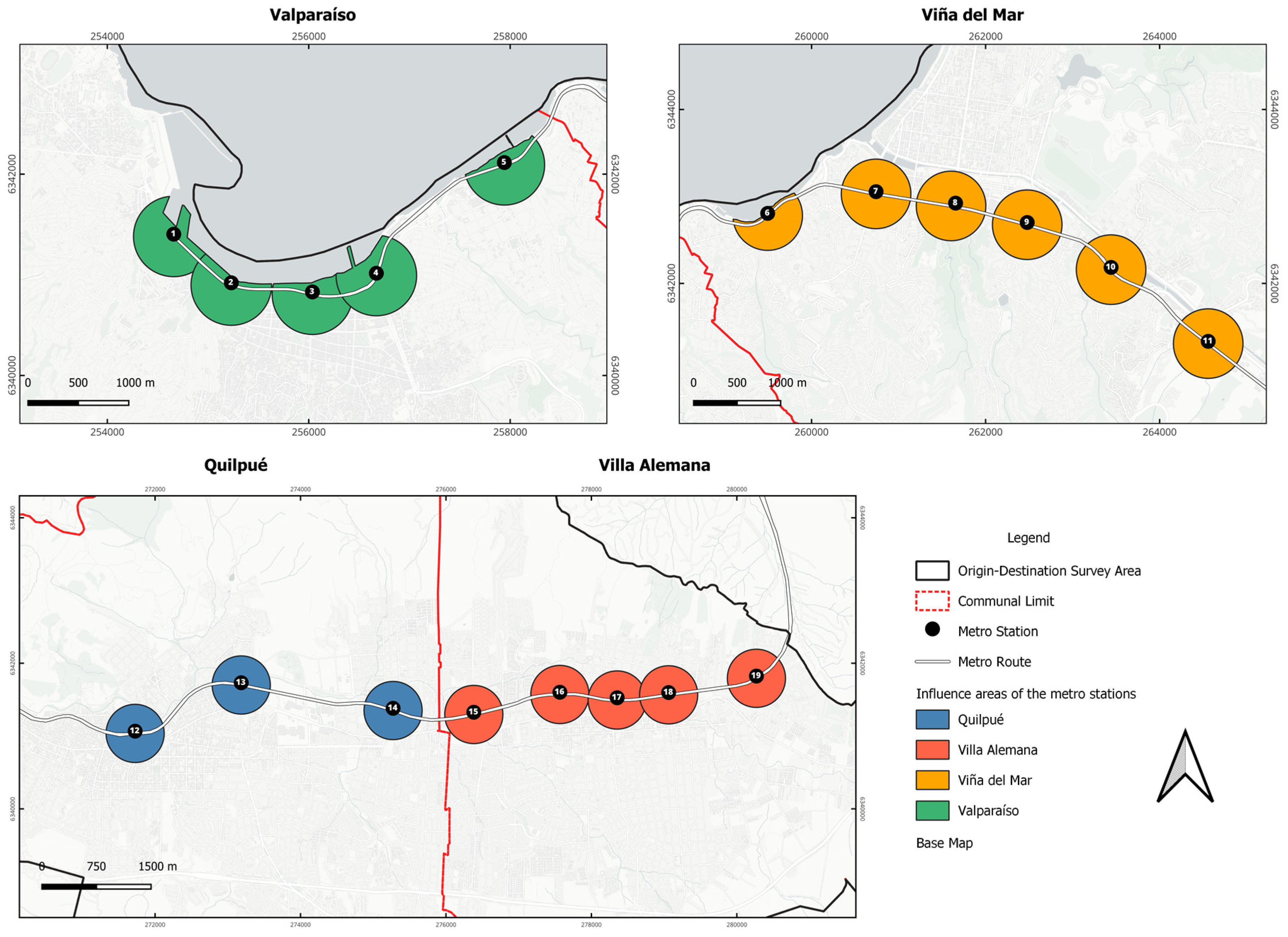
The first areas obtained using a 400-m radius buffer are presented in Figure 7. Each of these areas corresponds to each of the 19 stations present in Greater Valparaíso. By applying a buffer to each station, the result is the same for all areas, without taking into account territorial or topographical limits. A clear example is the stations located on the coast (Valparaíso stations and the first station in Viña del Mar), which cover areas through which people do not commonly circulate, such as the sea. In other areas, it can also cover areas where people do not live or circulate since this method generates a circumference around a point without considering external factors. Another important point is that, in this case, the 400-m areas may overlap in some stations, as can be seen on the map of Valparaíso and Villa Alemana. However, as mentioned before, this defined area of 400 m was chosen to avoid too much overlapping between stations.
The urban indicators within these 19 areas show an average density of 26.69 households per hectare, with notable variability for density and housing with respect to the standard deviation and the minimum and maximum values. In terms of road safety, design street safety has a low average of 0.1 vehicle accidents per hectare but with significant variability. Street design exhibits low variability, with an average of 1.75 Number of Nodes per Number of Streets. Mixed land (diversity) shows high consistency in the proportion of residential areas. In terms of accessibility, destination achieves an average walk score of 79.89, which is classified as “Very Walkable” [49]. Finally, the average distance to bus stops from the station is 85.4 m, but with high variability, reaching up to 405.07 m between zones (see Table 6). See Table A3 in the Appendix A for more information on the values of the urban environment indicators of the 19 areas.

5.2. Areas Reclassified and Vectorized Using KDE

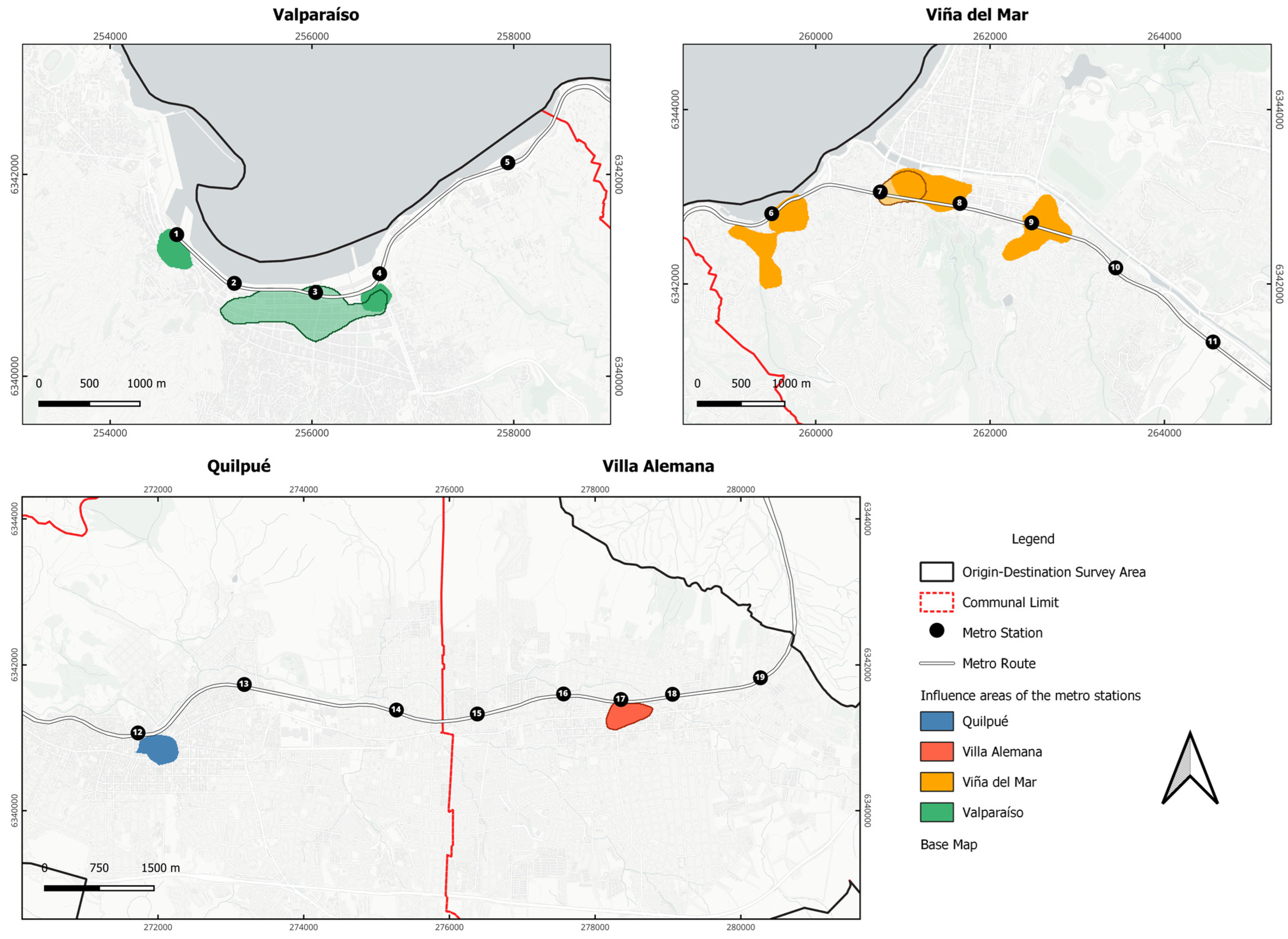
Figure 8 shows the result of the areas obtained from hotspot identification using KDE and subsequent reclassification and vectorization. In this case, areas more in line with the territory are observed since they are built from points that represent the origin of people who go to an area of 250 m radius from the stations. Therefore, they cover more habitable areas and/or are passable by people, resulting in different areas for each station.
The urban indicators of these nine areas show an average density of 39.64 housing units per hectare, with notable variability for density and housing, much higher compared to the 19 areas. Street safety has a higher average of 0.27 vehicle accidents per hectare, with significant variability. Street design exhibits low variability with a mean of 1.9, representing a low comparison with the 19 areas. Mixed land (diversity) shows a higher proportion of residential areas. In terms of accessibility, destination achieves an average walk score of 93.33, classified as “Walker’s Paradise” [49]. Finally, the average distance to bus stops is much greater, reaching 106.31 m, and less variability, reaching up to 210 m between zones (see Table 7). See Table A4 in the Appendix A for more information on the values of the urban environment indicators of the nine areas.

5.3. Model Results

Ordinary Least Squares (OLS) regression models were employed to explore the relationship between metro station ridership and various built environment variables between 2018 and 2023, utilizing two different methodologies for defining the influence areas of metro stations: one encompassing nine stations and another covering 19 stations. The models aimed to gauge the impact of factors such as density, design, destination, distance, and diversity on ridership numbers.
The analysis of the models’ fit over the years highlights a distinct pattern in relation to the pandemic’s impact on metro ridership. Notably, the models for the pre-pandemic year 2018 and the post-pandemic year 2023 demonstrate superior fits, indicating a strong relationship between the built environment variables and ridership levels during these periods. However, the model fits for the years 2019 and 2020 present a decline in the statistical significance, suggesting that the disruptions caused by the pandemic likely introduced anomalies in ridership behaviors. The years 2021 and 2022, while still impacted by pandemic-related factors, show a marginal improvement in model fit compared to the peak pandemic years, suggesting a gradual return toward normalcy in ridership patterns as the effects of the pandemic began to wane. For these reasons, only the models for 2018 and 2023, which demonstrated the best performance in terms of explanatory power, are analyzed.
Table 8 and Table 9 present the results of the models estimated for the nine stations in 2018 and 2023. The 2018 model for the nine stations showed a strong fit with an R2 of 0.877 and an adjusted R2 of 0.792, indicating a high explanatory power level. The model had 10 degrees of freedom and an F-value of 10.27, significant at a p-value of 0.0007. Among the variables, density and design related to street safety, as well as the distance from the nearest bus stops, showed positive and significant effects. In contrast, the destination accessibility (destination) variable was significant but negatively associated with ridership. Variables like diversity of land use, street design, and seasonal variation (vacation) were not statistically significant.
In 2023, the model exhibited a slight improvement in fit, with an R2 of 0.8798 and an adjusted R2 of 0.7957. The model’s structure remained consistent with 10 degrees of freedom and an F-value of 10.46, significant at a p-value of 0.00067. This model identified an additional significant variable, vacation, which negatively affected ridership while maintaining the significant impacts of the previously identified variables.
The estimation results of OLS regression for the 19 stations for 2018 and 2023 are presented in Table 10 and Table 11, respectively. The model representing the 19 stations in 2018 demonstrated a moderate explanatory power with an R2 of 0.5315 and an adjusted R2 of 0.4221. The only significant predictor was street safety, which had a positive impact on ridership. Other variables, including density, street design, diversity, and vacation, did not reach statistical significance.
For the year 2023, the model’s fit improved, with an R2 of 0.658 and an adjusted R2 of 0.5782. Similar to 2018, the only statistically significant variable was street safety. The improved fit suggests a better capture of ridership behavior over time, though the low number of significant predictors indicates potential oversimplification in the model or variation in data sensitivity.
In addition to the previous models and to complement the comparison process between the two methodologies, a regression model using only the nine fixed-radius influence areas corresponding to the set of OD-survey-based areas was estimated. This approach allows for a direct comparison by maintaining a consistent number of areas between the models. Table 12 presents the results of the models estimated for the equivalent 9 out of 19 fixed-radius influence areas. The results can be compared to the model of Table 9, highlighting the differences in explanatory power and significance of the variables.
The model presented in Table 9, based on the nine fixed-radius influence areas, showed a robust fit with an R2 of 0.8798 and an adjusted R2 of 0.7957, indicating a high level of explanatory power. The model had ten degrees of freedom and an F-value of 10.46, significant at a p-value of 0.0006779. Key findings from this model include a significant and positive effect of density with a coefficient of 7232 (p = 0.03247), a non-significant effect of street design with a coefficient of −53,602 (p = 0.86642), a significant and positive effect of street safety with a coefficient of 6,948,977 (p = 0.00198), a significant and negative effect of destination with a coefficient of −58,694 (p = 0.03815), a significant and positive effect of distance with a coefficient of 6719 (p = 0.03695), a non-significant effect of diversity with a coefficient of −1,308,596 (p = 0.40602), and a highly significant and negative effect of vacation with a coefficient of −664,720 (p = 4.29 × 10⁻⁵).
The model presented in Table 12, using the same nine influence areas of Table 9 but based on the fixed influence area, exhibited a slightly improved fit. This model had an R2 of 0.8848 and an adjusted R2 of 0.8042. It also had ten degrees of freedom and an F-value of 10.98, significant at a p-value of 0.0005545. In this model, density was not significant, with a negative coefficient of −3874 (p = 0.0936), street design was approaching significance with a coefficient of −553,042 (p = 0.0788), street safety was significant and positive with a coefficient of 3,521,673 (p = 0.0113), destination was not significant with a coefficient of −16,353 (p = 0.3192), distance was not significant with a coefficient of 2360 (p = 0.2889), diversity was significant and negative with a coefficient of −2,027,237 (p = 0.0385), and vacation was highly significant and negative with a coefficient of −664,720 (p = 3.59 × 10⁻⁵).
The comparison between the two models reveals differences. Table 9 model identifies density, destination, design (street safety), and distance as significant variables. Conversely, diversity is significant in Table 12 but not in Table 9. Both models agree on the significance of street safety and vacation, with vacation being consistently highly significant and negative. Table 12 demonstrates a slightly better overall fit, as indicated by the higher R2 and adjusted R2 values, lower residual standard error (200,600 vs. 204,900), and higher F-statistic. These differences highlight the impact of the number of areas of influence on the performance and explanatory power of the regression models. In conclusion, the choice between the two models depends on the research priorities: the model from Table 9 may be preferred for its number of significant variables, while the Table 12 model offers a slightly better overall fit and explanatory power.
The comparative analysis of the two influence area methodologies reveals that the models applied to the newly defined influence areas provided a consistent model and a higher number of significant explanatory variables. This suggests that the model based on the OD survey data for defining station influence areas may better represent the complexities of the built environment’s impact on metro ridership. This finding aligns with previous research indicating that station-specific characteristics and surroundings can significantly influence ridership levels.

6. Conclusions

Regarding the different influence area approaches, it is possible to note that an in-fluence area defined by the “real” use of the metro station’s surroundings, based on an origin and destination survey, generates better analytical conditions with respect to the relation between the built environment and metro ridership. Therefore, it is relevant to question whether a fixed distance radius from metro stations is adequate to evaluate the impact of the urban and transport characteristics of its surroundings on its ridership.
Furthermore, the results show that the land use mix and street design did not present a representative statistical explanation for the metro ridership, as expected from a TOD-designed area, except for the density indicator. In addition, from the statistically relevant indicators, there are some inverse results that would be expected from a TOD-planned area. For example, the higher the number of accidents harming pedestrians leads to higher metro ridership; the increased walkability at the influence area reduces the use of the metro system; and longer distances to bus stops promote higher metro ridership.
In light of this analysis, it is possible to confirm that the metro and bus systems in Greater Valparaíso are competing with each other instead of promoting intermodal mobility. Also, the level of walkability to a diversity of services around metro stations relates negatively to metro ridership, and people are conditioned to be exposed to accidents around metro stations, meaning that there may not be alternatives to avoid this exposure.
In general, this study indicates that the metro system in Greater Valparaíso was not planned in synergy with the urban development of this metropolitan area. This may connect to the challenges regarding a change of transport planning perspective toward a sustainable approach. As discussed by Banister [64], there is a need to confront two traditional dilemmas of transport planning: (1) Transport as a derived demand or as a valued activity; (2) Time minimization or reasonable travel time. These questions related directly to the lack of consideration of the urban characteristics and necessities of people regarding public transport projects.
In this direction, this study is an initial diagnostic of the relationship between the built environment and metro ridership in the metropolitan area of Valparaíso and opens new questions about specific aspects of the metro system and its relationship to its surroundings. For future studies, it is recommended to explore the effects of sociodemographic factors and more detailed built environment factors, such as conditions of public spaces and the presence of universal accessibility infrastructure, on the system’s ridership and accessibility to the metro stations.

Author Contributions

Conceptualization, Vicente Aprigliano, Sebastian Seriani, and Cristo Cucumides; methodology, Vicente Aprigliano, Sebastian Seriani, Catalina Toro, Gonzalo Rojas, and Mitsuyoshi Fukushi; validation, Vicente Aprigliano, Sebastian Seriani, and Cristo Cucumides; formal analysis, Vicente Aprigliano, Sebastian Seriani, Catalina Toro, Gonzalo Rojas, Mitsuyoshi Fukushi, and Cristo Cucumides; investigation, Vicente Aprigliano, Sebastian Seriani, Catalina Toro, Gonzalo Rojas, Mitsuyoshi Fukushi, and Cristo Cucumides; data curation, Catalina Toro, Gonzalo Rojas, and Mitsuyoshi Fukushi; writing—original draft preparation, Vicente Aprigliano, Sebastian Seriani, Catalina Toro, Gonzalo Rojas, Mitsuyoshi Fukushi, Cristo Cucumides, Marcus Cardoso, Marcelino Aurelio Vieira da Silva, Ualison Rébula de Oliveira, Cristián Henríquez, Andreas Braun, and Volker Hochschild; writing—review and editing, Vicente Aprigliano, Sebastian Seriani, Catalina Toro, Gonzalo Rojas, Mitsuyoshi Fukushi, Cristo Cucumides, Marcus Cardoso, Marcelino Aurelio Vieira da Silva, Ualison Rébula de Oliveira, Cristián Henríquez, Andreas Braun, and Volker Hochschild; visualization, Vicente Aprigliano, Sebastian Seriani, Catalina Toro, Gonzalo Rojas, and Mitsuyoshi Fukushi; supervision, Vicente Aprigliano; project administration, Vicente Aprigliano, and Sebastian Seriani; funding acquisition, Vicente Aprigliano and Sebastian Seriani. All authors have read and agreed to the published version of the manuscript.

Funding

This research was funded by Agencia Nacional de Investigación y Desarrollo (ANID), Chile, grant number 11230050, ID22I10018, 1220688, and 1522A0002.

Data Availability Statement

No new data were created or analyzed in this study. Data sharing is not applicable to this article.

Acknowledgments

This study is supported by FONDECYT Project 11230050, FONDEF Project ID22I10018, FONDECYT Project 1220688, and FONDAP 1522A0002, all from Agencia Nacional de Investigación y Desarrollo (ANID), Chile.

Conflicts of Interest

The authors declare no conflict of interest.

Appendix A

Table A1. Methodological summary for urban environment indicators. Source: elaborated by Authors.
DimensionIndicatorsMethodologyEquations
DensityHousingUsing the 2017 Census shapefile, the total number of homes was calculated and divided into the area of the municipality expressed in hectares (ha). T o t a l   H o u s i n g   u n i t T o t a l   a r e a   ( h a )
DesignStreet designUsing the street network, the calculation of nodes was carried out with a Qgis geoprocessing tool, making a sum of their total. Dividing it into the total number of streets, considering them topologically. T o t a l   N u m b e r   o f   N o d e s T o t a l   N u m b e r   o f   T o p o l o g i c a l   S t r e e t s
Street safetyThe sum of the total number of vehicle accidents per area was made, and then the proportion was obtained by dividing it by the total area expressed in hectares. T o t a l   N u m b e r   o f   v e h i c u l a r   a c c i d e n t s T o t a l   a r e a   ( h a )
DestinationWalkscoreUsing Python and the pandas, geopandas, requests, json, and urllib.parse libraries. Two functions were generated. The first of them, called “address”, receives a pair of geographical coordinates and, by connecting to the Nominatum API, converts them into the address format required by the Walkscore API. The second function, called “walkscore”, receives a polygon in shapefile format, extracts its centroid and uses this pair of coordinates as input to the “direct” function. This generates the URL needed to enter the Walkscore API and obtain the score provided by Walkscore.Functions:
direc(lat,lon) = address in format required by walkscore.
Walkscore(polygon) = Walkscore
DistanceDistance to the nearest bus stopGoogle Maps was used to generate the shortest route between the metro station and a bus stop within the area.Real distance calculation using Google Maps
DiversityMixed land Using the PRC shapefile from the municipalities of Valparaíso, Viña del Mar, Quilpué, and Villa Alemana. It was filtered by the residential areas, adding the total area of these to divide it into the total area, expressed in hectares (ha). T o t a l   R e s i d e n t i a l   a r e a   ( h a ) T o t a l   a r e a   ( h a )
Table A2. Methodological summary and formulas for calculating socioeconomic characteristics of the municipalities. To calculate the characteristics described in the table, the data available in the origin and destination survey were used. Source: elaborated by Authors.
CharacteristicsMethodologyEquationsExplanation
Total PopulationSum of the expansion factor of each person present in the municipality. i = 1 N w i N :   Total   number   of   people
w i :   Expansion   factor   associated   with   the   unit   of   persons   i
Ratio of women to total populationRelationship of the sum of the expansion factor of women in the municipality and the sum of the expansion factor of the population of the municipality. i = 1 N ( w i f i ) i = 1 N w i N :   Total   number   of   people
f i :   1 : g e n d e r i = f e m a l e 0 : g e n d e r i f e m a l e
w i :   Expansion   factor   associated   with   the   unit   of   persons   i
Average ageRelationship of the sum of the age of each person by their municipality expansion value and the sum of the total expansion factor of the municipality’s population. i = 1 N ( w i x i ) i = 1 N w i N :   Total   number   of   people
x i :   Age   of   unit   i
w i :   Expansion   factor   associated   with   the   unit   of   persons   i
Houlsehold SizeRelationship of the sum of the expansion factor of people in the municipality and the sum of the total expansion factor of households in the municipality. i = 1 N w i P e r s o n j = 1 M w j H o u l s e h o l d N :   Total   number   of   people
M :   Total   number   of   houlseholds
w i P e r s o n :   Expansion   factor   associated   with   the   unit   of   persons   i
w j H o u l s e h o l d :   Expansion   factor   associated   with   the   unit   of   households   j
Cars per householdRelationship of the sum of the expansion factor of households with cars and the sum of the expansion factor of households in the municipality. j = 1 N ( w j x j ) j = 1 M w j N :   Total   number   of   people
M :   Total   number   of   households
x j :   1 : C a r s   p e r   h o u s e h o l d i = T r u e   0 :   C a r s   p e r   h o u s e h o l d i = F a l s e  
w j :   Expansion   factor   associated   with   the   unit   of   households   j
Household incomeRelationship of the sum of the product of the income of a household j by the household expansion factor and the sum of the household expansion factor in the municipality. j = 1 N ( w j x j ) j = 1 N w j N :   Total   number   of   people
x j :   Household   income   of   unit   j
w j :   Expansion   factor   associated   with   the   unit   of   households   j
Population in need of careRelationship of the sum of the person expansion factor for those younger than 14 years old and those older or equal to 60 years old, and the sum of the expansion factor of the population of the municipality. i = 1 N ( w i x i ) i = 1 N w i N :   Total   number   of   people
x i :   1 : a g e i   14   or     a g e i     60   0 : a g e i > 14         a g e i < 60  
w i :   Expansion   factor   associated   with   the   unit   of   persons   i
Primary educationRelationship of the sum of the product between those people over 18 years of age who do not study and who have completed primary education (x = 1) by their associated expansion factor and the sum of the expansion factor of the population older than 18 years of the municipality. i = 1 N ( w i x i ) i = 1 N ( w i y i ) N :   Total   number   of   people
x i :   I f   a g e i     18   a c t i v i t y i ≠ study ∧ e d u c a t i o n i = Primary
y i : a g e i     18  
w i :   Expansion   factor   associated   with   the   unit   of   persons   i
Secundary educationRelationship of the sum of the product between those people over 18 years of age who do not study and who have completed secondary education (x = 1) by their associated expansion factor and the sum of the expansion factor of the equal and older population than 18 years old from the municipality. i = 1 N ( w i x i ) i = 1 N ( w i y i ) N :   Total   number   of   people
x i :   I f   a g e i     18   a c t i v i t y i ≠ study ∧ e d u c a t i o n i = Secundary
y i : a g e i     18  
w i :   Expansion   factor   associated   with   the   unit   of   persons   i
Superior educationRelationship of the sum of the product between those people over 29 years of age who do not study and who have completed higher education (x = 1) by their associated expansion factor and the sum of the expansion factor of the equal and older population than 29 years old from the municipality. i = 1 N ( w i x i ) i = 1 N ( w i y i ) N :   Total   number   of   people
x i :   I f   a g e i     29   a c t i v i t y i ≠ study ∧ e d u c a t i o n i = Superior
y i : a g e i     29  
w i :   Expansion   factor   associated   with   the   unit   of   persons   i
WorkersRelationship of the sum of the product of people over 15 years of age who work and who are not under 18 years of age studying (x = 1) and the sum of the household expansion factor. i = 1 N ( w i P e r s o n x i ) j = 1 M w j H o u l s e h o l d   N :   Total   number   of   people
M :   Total   number   of   houlsehold
x i :   a g e i ≥ 15 ∧ a c t i v i t y i = work     ( a g e i > 18 ∧ a c t i v i t y i ! = study )
w i P e r s o n :   Expansion   factor   associated   with   the   unit   of   persons   i
w j H o u l s e h o l d :   Expansion   factor   associated   with   the   unit   of   households   i
Car driving licenseRelationship of the sum of the product of people with a driver’s license (x = 1) by their associated expansion factor and the sum of the household expansion factor. i = 1 N ( w i P e r s o n x i ) j = 1 M w j H o u l s e h o l d   N :   Total   number   of   people
M :   Total   number   of   houlseholds
x i :   d r i v i n g   l i c e n s e i   = Car   driving   license
w i P e r s o n :   Expansion   factor   associated   with   the   unit   of   persons   i
w j H o u l s e h o l d :   Expansion   factor   associated   with   the   unit   of   households   i
Households with bicyclesRelationship of the sum of the product of households with at least one bicycle (x = 1) by its associated expansion factor and the sum of the expansion factor of households. j = 1 N ( w j x j ) j = 1 M w j N :   Total   number   of   people
M :   Total   number   of   households
x j :   H o u s e h o l d s   w i t h   b i c y c l e s i   = True
w j :   Expansion   factor   associated   with   the   unit   of   households   j
Table A3. Total score of urban environment indicators within areas of 400 m radius. Source: elaborated by authors.
StationsDensity: HousingDesign: Street SafetyDesign: Street DesignDiversity: Mixed LandDestination: WalkScoreDistance: to the Nearest Bus Stop
Puerto20.120.192.070.759939.84
Bellavista26.910.312.130.8710052.18
Francia20.800.242.171.009779.71
Barón24.600.101.750.929333.00
Portales23.650.081.400.7382100.00
Recreo35.150.031.830.958464.00
Miramar75.160.131.850.819899.00
Viña del Mar40.110.241.620.9399120.00
Hospital81.210.171.920.858916.4
Chorrillos26.200.051.660.827343.87
El Salto0.990.020.600.913748.66
Quilpué13.250.161.620.878969.23
El Sol16.630.001.790.8463405.07
El Belloto15.770.061.920.906879.7
Las Américas21.130.031.560.9653196.85
La Concepción18.490.011.830.957639.77
Villa Alemana13.280.112.070.938657.67
Sargento Aldea17.300.021.830.957918.25
Peñablanca16.430.011.671.005359.33
Table A4. Total score of urban environment indicators within areas reclassified and vectorized using KDE. Source: elaborated by authors.
StationsDensity: HousingDesign: Street SafetyDesign: Street DesignDiversity: Mixed LandDestination: WalkScoreDistance: to the Nearest Bus Stop
Puerto17.120.4217.960.899939.84
Francia29.320.3322.380.989879.71
Barón9.130.2813.87195128.32
Recreo34.360.0316.090.9884210
Miramar106.840.2520.71199110
Viña del Mar69.130.3118.170.9499120
Hospital68.50.2418.350.768916.4
Quilpué14.020.2815.94190159.4
Villa Alemana8.340.2518.480.988793.12

References

  1. To, W.M.; Lee, P.K.C.; Yu, B.T.W. Sustainability Assessment of an Urban Rail System—The Case of Hong Kong. J. Clean. Prod. 2020, 253, 119961. [Google Scholar] [CrossRef]
  2. Lin, D.; Broere, W.; Cui, J. Metro Systems and Urban Development: Impacts and Implications. Tunn. Undergr. Space Technol. 2022, 125, 104509. [Google Scholar] [CrossRef]
  3. Patnala, P.K.; Parida, M.; Chalumuri, R.S. Gender Differentials in Travel Behavior among TOD Neighborhoods: Contributions of Built Environment and Residential Self-Selection. Travel Behav. Soc. 2023, 31, 333–348. [Google Scholar] [CrossRef]
  4. Xia, J.; Zhang, Y. Where Are Potential Areas for Transit-Oriented Development (TOD)—Exploring the Demands for Built Environment for TOD Planning. Sustainability 2022, 14, 8364. [Google Scholar] [CrossRef]
  5. Huang, J.; Chen, S.; Xu, Q.; Chen, Y.; Hu, J. Relationship between Built Environment Characteristics of TOD and Subway Ridership: A Causal Inference and Regression Analysis of the Beijing Subway. J. Rail Transp. Plan. Manag. 2022, 24, 100341. [Google Scholar] [CrossRef]
  6. Deng, X.; Zhang, J.; Liao, S.; Zhong, C.; Gao, F.; Teng, L. Interactive Impacts of Built Environment Factors on Metro Ridership Using GeoDetector: From the Perspective of TOD. ISPRS Int. J. Geo-Inf. 2022, 11, 623. [Google Scholar] [CrossRef]
  7. Wey, W.-M.; Zhang, H.; Chang, Y.-J. Alternative Transit-Oriented Development Evaluation in Sustainable Built Environment Planning. Habitat Int. 2016, 55, 109–123. [Google Scholar] [CrossRef]
  8. Wey, W.-M.; Chiu, Y.-H. Assessing the Walkability of Pedestrian Environment under the Transit-Oriented Development. Habitat Int. 2013, 38, 106–118. [Google Scholar] [CrossRef]
  9. Elgohary, M.M.; Abdin, A.R.; Khalil, H.A.E. Upgrading Informal Areas through Sustainable Urban Development Principles. J. Eng. Appl. Sci. 2024, 71, 65. [Google Scholar] [CrossRef]
  10. Ibraeva, A.; Correia, G.H.D.A.; Silva, C.; Antunes, A.P. Transit-Oriented Development: A Review of Research Achievements and Challenges. Transp. Res. Part A Policy Pract. 2020, 132, 110–130. [Google Scholar] [CrossRef]
  11. Cervero, R.; Sarmiento, O.L.; Jacoby, E.; Gomez, L.F.; Neiman, A. Influences of Built Environments on Walking and Cycling: Lessons from Bogotá. Int. J. Sustain. Transp. 2009, 3, 203–226. [Google Scholar] [CrossRef]
  12. Manville, M. Travel and the Built Environment: Time for Change. J. Am. Plan. Assoc. 2017, 83, 29–32. [Google Scholar] [CrossRef]
  13. Wu, B.M.; Hine, J.P. A PTAL Approach to Measuring Changes in Bus Service Accessibility. Transp. Policy 2003, 10, 307–320. [Google Scholar] [CrossRef]
  14. Qureshi, S.; Memon, I.A.; Talpur, M.A.H. Association between Objectively Measured Neighbourhood Built Environment and Walkability. Mehran Univ. Res. J. Eng. Technol. 2022, 41, 157–168. [Google Scholar] [CrossRef]
  15. Gori, S.; Nigro, M.; Petrelli, M. Walkability Indicators for Pedestrian-Friendly Design. Transp. Res. Rec. 2014, 2464, 38–45. [Google Scholar] [CrossRef]
  16. Hollenstein, D.; Bleisch, S. Walkability for Different Urban Granularities. Int. Arch. Photogramm. Remote Sens. Spat. Inf. Sci. 2016, XLI-B2, 703–708. [Google Scholar] [CrossRef]
  17. Erath, A.; Van Eggermond, M.A.B.; Ordóñez, S.A.; Axhausen, K.W. Introducing the Pedestrian Accessibility Tool: Walkability Analysis for a Geographic Information System. Transp. Res. Rec. 2017, 2661, 51–61. [Google Scholar] [CrossRef]
  18. Lefebvre-Ropars, G.; Morency, C. Walkability: Which Measure to Choose, Where to Measure It, and How? Transp. Res. Rec. 2018, 2672, 139–150. [Google Scholar] [CrossRef]
  19. Lin, Y.-P.; Chu, H.-J.; Wu, C.-F.; Chang, T.-K.; Chen, C.-Y. Hotspot Analysis of Spatial Environmental Pollutants Using Kernel Density Estimation and Geostatistical Techniques. Int. J. Environ. Res. Public Health 2010, 8, 75–88. [Google Scholar] [CrossRef]
  20. SECTRA. ENCUESTAS DE MOVILIDAD. Available online: https://www.sectra.gob.cl/encuestas_movilidad/encuestas_movilidad.htm (accessed on 24 April 2024).
  21. EFE. Plan Marzo: EFE Valparaíso Anuncia Aumento de Capacidad de Transporte a Partir Del 1 de Marzo—EFE Trenes de Chile. Available online: https://www.efe.cl/plan-marzo-efe-valparaiso-anuncia-aumento-de-capacidad-de-transporte-a-partir-del-1-de-marzo/ (accessed on 24 April 2024).
  22. Aprigliano, V.; Barros, G.T.; Santos, M.V.S.M.; Toro, C.; Rojas, G.; Seriani, S.; Da Silva, M.A.V.; De Oliveira, U.R. Sustainable Mobility Challenges in the Latin American Context. Sustainability 2023, 15, 14748. [Google Scholar] [CrossRef]
  23. Parra, María del Mar Retrocede el Nuevo Plan Regulador de Valparaíso por No Considerar Amenazas Ambientales. Available online: https://www.eldesconcierto.cl/bienes-comunes/2023/10/31/retrocede-el-nuevo-plan-regulador-de-valparaiso-por-no-considerar-amenazas-ambientales.html (accessed on 24 April 2024).
  24. Consejo Políticas de Infraestructura Zoom a los Planes Reguladores Comunales e Intercomunales: “El Diagnóstico No es el Mejor.” CPI 2023. Available online: https://www.infraestructurapublica.cl/zoom-a-los-planes-reguladores-comunales-e-intercomunales-el-diagnostico-no-es-el-mejor/ (accessed on 24 April 2024).
  25. El Observador En 2024 Estarían Listos Los Diseños Del Tren Hasta La Calera. Available online: https://www.observador.cl/en-2024-estarian-listos-los-disenos-del-tren-hasta-la-calera/ (accessed on 24 April 2024).
  26. Taylor, B.D.; Fink, C.N.Y. Explaining Transit Ridership: What Has the Evidence Shown? Transp. Lett. 2013, 5, 15–26. [Google Scholar] [CrossRef]
  27. Hasnine, M.S.; Hawkins, J.; Habib, K.N. Effects of Built Environment and Weather on Demands for Transportation Network Company Trips. Transp. Res. Part A Policy Pract. 2021, 150, 171–185. [Google Scholar] [CrossRef]
  28. An, R.; Zahnow, R.; Pojani, D.; Corcoran, J. Weather and Cycling in New York: The Case of Citibike. J. Transp. Geogr. 2019, 77, 97–112. [Google Scholar] [CrossRef]
  29. Böcker, L.; Priya Uteng, T.; Liu, C.; Dijst, M. Weather and Daily Mobility in International Perspective: A Cross-Comparison of Dutch, Norwegian and Swedish City Regions. Transp. Res. Part D Transp. Environ. 2019, 77, 491–505. [Google Scholar] [CrossRef]
  30. Tao, S.; Corcoran, J.; Rowe, F.; Hickman, M. To Travel or Not to Travel: ‘Weather’ Is the Question. Modelling the Effect of Local Weather Conditions on Bus Ridership. Transp. Res. Part C Emerg. Technol. 2018, 86, 147–167. [Google Scholar] [CrossRef]
  31. Wei, M. How Does the Weather Affect Public Transit Ridership? A Model with Weather-Passenger Variations. J. Transp. Geogr. 2022, 98, 103242. [Google Scholar] [CrossRef]
  32. Kim, Y.; Kim, E.-J.; Jang, S.; Kim, D.-K. A Comparative Analysis of the Users of Private Cars and Public Transportation for Intermodal Options under Mobility-as-a-Service in Seoul. Travel Behav. Soc. 2021, 24, 68–80. [Google Scholar] [CrossRef]
  33. Long, A.; Carney, F.; Kandt, J. Who Is Returning to Public Transport for Non-Work Trips after COVID-19? Evidence from Older Citizens’ Smart Cards in the UK’s Second Largest City Region. J. Transp. Geogr. 2023, 107, 103529. [Google Scholar] [CrossRef] [PubMed]
  34. Li, M.; Kwan, M.-P.; Hu, W.; Li, R.; Wang, J. Examining the Effects of Station-Level Factors on Metro Ridership Using Multiscale Geographically Weighted Regression. J. Transp. Geogr. 2023, 113, 103720. [Google Scholar] [CrossRef]
  35. Curtis, C. Delivering the “D” in Transit-Oriented Development: Examining the Town Planning Challenge. J. Transp. Land Use 2012, 5, 83–99. [Google Scholar] [CrossRef]
  36. Sohn, K.; Shim, H. Factors Generating Boardings at Metro Stations in the Seoul Metropolitan Area. Cities 2010, 27, 358–368. [Google Scholar] [CrossRef]
  37. Ramos-Santiago, L.E. Does Walkability around Feeder Bus-Stops Influence Rapid-Transit Station Boardings? J. Public Transp. 2022, 24, 100026. [Google Scholar] [CrossRef]
  38. Gan, Z.; Feng, T.; Yang, M.; Timmermans, H.; Luo, J. Analysis of Metro Station Ridership Considering Spatial Heterogeneity. Chin. Geogr. Sci. 2019, 29, 1065–1077. [Google Scholar] [CrossRef]
  39. Jun, M.-J.; Choi, K.; Jeong, J.-E.; Kwon, K.-H.; Kim, H.-J. Land Use Characteristics of Subway Catchment Areas and Their Influence on Subway Ridership in Seoul. J. Transp. Geogr. 2015, 48, 30–40. [Google Scholar] [CrossRef]
  40. Zhao, P.; Li, S. Bicycle-Metro Integration in a Growing City: The Determinants of Cycling as a Transfer Mode in Metro Station Areas in Beijing. Transp. Res. Part A Policy Pract. 2017, 99, 46–60. [Google Scholar] [CrossRef]
  41. Nyunt, K.T.K.; Wongchavalidkul, N. Evaluation of Relationships between Ridership Demand and Transit-Oriented Development (TOD) Indicators Focused on Land Use Density, Diversity, and Accessibility: A Case Study of Existing Metro Stations in Bangkok. Urban Rail Transit 2020, 6, 56–70. [Google Scholar] [CrossRef]
  42. He, Y.; Zhao, Y.; Tsui, K.-L. Geographically Modeling and Understanding Factors Influencing Transit Ridership: An Empirical Study of Shenzhen Metro. Appl. Sci. 2019, 9, 4217. [Google Scholar] [CrossRef]
  43. Gupta, A.; Bivina, G.R.; Parida, M. Does Neighborhood Design Matter for Walk Access to Metro Stations? An Integrated SEM-Hybrid Discrete Mode Choice Approach. Transp. Policy 2022, 121, 61–77. [Google Scholar] [CrossRef]
  44. Liu, X.; Chen, X.; Tian, M.; De Vos, J. Effects of Buffer Size on Associations between the Built Environment and Metro Ridership: A Machine Learning-Based Sensitive Analysis. J. Transp. Geogr. 2023, 113, 103730. [Google Scholar] [CrossRef]
  45. Li, S.; Yang, H.; Zhang, G.; Ling, Z.; Xiong, Y.; Li, Y. What Is the Best Catchment Area of a Metro Station? A Study Based on Station Level Ridership Modeling. In Proceedings of the 2019 5th International Conference on Transportation Information and Safety (ICTIS), Liverpool, UK, 14–17 July 2019; pp. 1239–1244. [Google Scholar]
  46. Biblioteca del Congreso Nacional Mapas Vectoriales. Available online: https://www.bcn.cl/siit/mapas_vectoriales/index_html (accessed on 24 April 2024).
  47. Comisión Nacional de Seguridad de Tránsito Comisión Nacional de Seguridad de Tránsito. Available online: https://mapas-conaset.opendata.arcgis.com/search?q=valparaiso (accessed on 24 April 2024).
  48. Okabe, A.; Satoh, T.; Sugihara, K. A Kernel Density Estimation Method for Networks, Its Computational Method and a GIS-based Tool. Int. J. Geogr. Inf. Sci. 2009, 23, 7–32. [Google Scholar] [CrossRef]
  49. WalkScore Walk Score API for Web and Mobile Developers. Available online: https://www.walkscore.com/professional/api.php (accessed on 24 April 2024).
  50. OpenStreetMap Nominatim. Available online: https://nominatim.org/ (accessed on 24 April 2024).
  51. Ministerio de Vivienda y Urbanismo Descarga IPT y Documentos. Available online: https://ide.minvu.cl/pages/descargas (accessed on 24 April 2024).
  52. Instituto Nacional de Estadísticas Microdatos Censo 2017: Manzana—Información General. Available online: https://ine-chile.maps.arcgis.com/home/item.html?id=54e0c40680054efaabeb9d53b09e1e7a (accessed on 24 April 2024).
  53. Motieyan, H.; Mesgari, M. Towards Sustainable Urban Planning Through Transit-Oriented Development (A Case Study: Tehran). ISPRS Int. J. Geo-Inf. 2017, 6, 402. [Google Scholar] [CrossRef]
  54. Zhang, Z.; Fisher, T.; Wang, H. Walk Score, Environmental Quality and Walking in a Campus Setting. Land 2023, 12, 732. [Google Scholar] [CrossRef]
  55. Google Maps Google Maps. Available online: https://www.google.com/maps/@-33.0432512,-71.6056975,15z?entry=ttu (accessed on 24 April 2024).
  56. Zhang, L.; Ye, Y.; Zeng, W.; Chiaradia, A. A Systematic Measurement of Street Quality through Multi-Sourced Urban Data: A Human-Oriented Analysis. Int. J. Environ. Res. Public Health 2019, 16, 1782. [Google Scholar] [CrossRef]
  57. Pongprasert, P.; Kubota, H. The Influences of Built Environment Factors on Mode Switching of TOD Residents from Car Use to Transit Dependence: Case Study of Bangkok, Thailand. In Proceedings of the International Conference on Transportation and Development 2018, Pittsburgh, PA, USA, 12 July 2018; pp. 186–197. [Google Scholar]
  58. Gutiérrez, J.; Cardozo, O.D.; García-Palomares, J.C. Transit Ridership Forecasting at Station Level: An Approach Based on Distance-Decay Weighted Regression. J. Transp. Geogr. 2011, 19, 1081–1092. [Google Scholar] [CrossRef]
  59. Zhao, J.; Deng, W.; Song, Y.; Zhu, Y. Analysis of Metro Ridership at Station Level and Station-to-Station Level in Nanjing: An Approach Based on Direct Demand Models. Transportation 2013, 41, 133–155. [Google Scholar] [CrossRef]
  60. Sung, H.; Oh, J.-T. Transit-Oriented Development in a High-Density City: Identifying Its Association with Transit Ridership in Seoul, Korea. Cities 2011, 28, 70–82. [Google Scholar] [CrossRef]
  61. Instituto Nacional de Estadísticas Instituto Nacional de Estadísticas|REDATAM Procesamiento y Diseminación. Available online: https://redatam-ine.ine.cl/redbin/RpWebEngine.exe/Portal?BASE=CENSO_2017&lang=esp (accessed on 24 April 2024).
  62. EFE Valparaiso. Memoria Anual 2020 XXVIII; EFE Valparaiso: Valparaiso, Chile, 2022. [Google Scholar]
  63. EFE Valparaiso Tren Limache–Puerto–EFE Trenes de Chile. Available online: https://www.efe.cl/nuestros-servicios/limache-puerto/ (accessed on 24 April 2024).
  64. Banister, D. The Sustainable Mobility Paradigm. Transp. Policy 2008, 15, 73–80. [Google Scholar] [CrossRef]
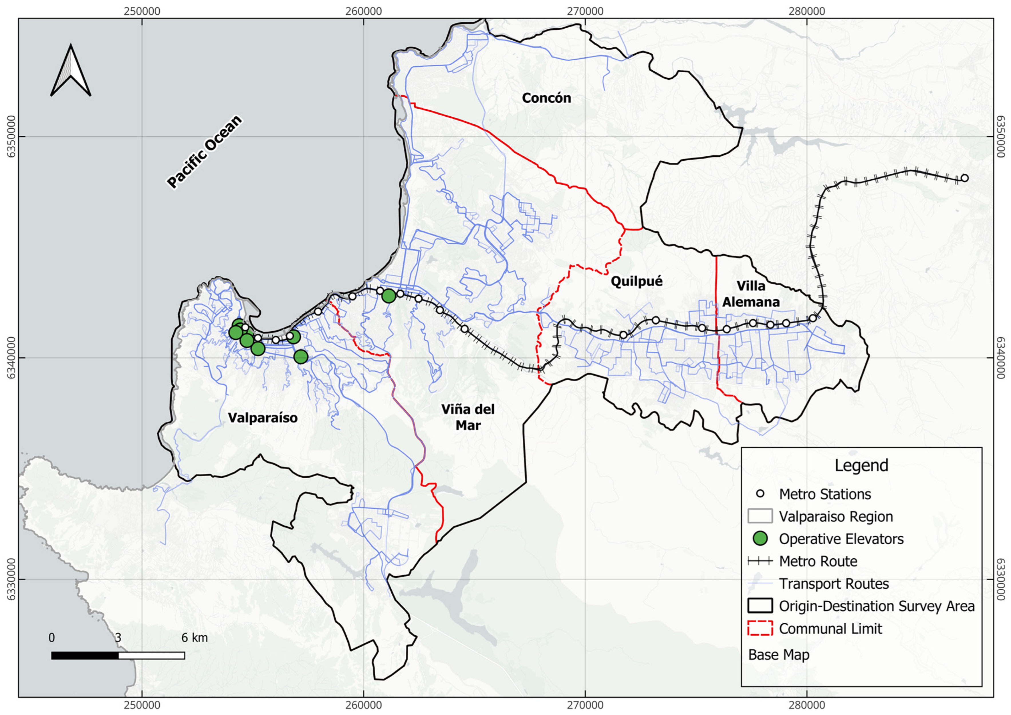
Figure 1. Transportation context in the Metropolitan Area of Valparaíso. Observation: the names on the map refer to the cities in the Metropolitan Area of Valparaíso. Source: Elaborated by authors.
Ijgi 13 00266 g001
Figure 2. EFE Valparaíso metro network and stations within the Greater Valparaíso. Observation: the names on the map refer to the cities in the Metropolitan Area of Valparaíso. Source: elaborated by authors.
Ijgi 13 00266 g002
Figure 3. Walkable influence areas of origin of people heading 250 m, 500 m, and 750 m from metro stations. Observation: the names on the map refer to the metro stations. Source: elaborated by authors.
Ijgi 13 00266 g003
Figure 4. Density of origin of people who go to an area of influence of 250 m from the metro stations of Greater Valparaíso by modal choice: (a) Walking; (b) Bicycle; (c) Public transport; (d) Private transport. Source: elaborated by authors.
Ijgi 13 00266 g004
Figure 5. (a) Annual metro passenger flow between the years 2018 and 2023 for the Greater Valparaíso area that covers the metro network. (b) Average annual flow in the metro stations of Greater Valparaíso for work and holiday months. Source: elaborated by authors.
Ijgi 13 00266 g005
Figure 6. Average passenger flow per month between 2018 and 2023, categorized by work and holiday months. Source: elaborated by authors.
Ijgi 13 00266 g006
Figure 7. Areas of influence of metro stations in Greater Valparaíso with a radius of 400 meters. Observation: the names on the top of each part of the figure refer to the city on the map. Source: elaborated by authors.
Ijgi 13 00266 g007
Figure 8. Influence areas of metro stations in Greater Valparaíso reclassified and vectorized using KDE. Observation: the names on the top of each part of the figure refer to the city on the map and the numbers refers to the information in Figure 2. Source: elaborated by authors.
Ijgi 13 00266 g008
Table 1. Pixel values with which the new areas of influence were obtained. The reclassification was carried out based on values equal to or greater than those described in the table. These areas will be presented in the Results section. Source: elaborated by authors.
MunicipalityStation NamePixel Value
ValparaísoPuerto1.77083 × 10−6
Francia5.10379 × 10−7
Barón1.29807 × 10−6
Viña del MarRecreo4.381 × 10−7
Miramar1.09325 × 10−6
Viña del Mar6.37435 × 10−7
Hospital5.64058 × 10−7
QuilpuéQuilpué7.15722 × 10⁻⁷
Villa AlemanaVilla Alemana6.71036 × 10−7
Table 2. Methodologies applied to obtain influence areas of metro stations. Source: Elaborated by authors.
IDStationNumber of PointsMethod 1Method 2
1Puerto>5Buffer (400 m)KDE- reclassified-vectorized
2Bellavista<5
3Francia>5KDE- reclassified-vectorized
4Barón=5KDE- reclassified-vectorized
5Portales<5
6Recreo=5KDE- reclassified-vectorized
7Miramar>5KDE- reclassified-vectorized
8Viña del Mar>5KDE- reclassified-vectorized
9Hospital>5KDE- reclassified-vectorized
10Chorrillos<5
11El Salto<5
12Quilpué=5KDE- reclassified-vectorized
13El Sol<5
14El Belloto<5
15Las Américas<5
16La Concepción<5
17Villa Alemana>5KDE- reclassified-vectorized
18Sargento Aldea<5
19Peñablanca<5
Table 4. Number of inhabitants in the municipalities of Greater Valparaíso. Source: elaborated by authors based on data from the National Institute of Statistics [61].
MunicipalityMaleFemaleTotal
Valparaíso144,945 (48.9%)151,710 (51.1%)296,655
Viña del Mar158,669 (47.5%)175,579 (52.5%)334,248
Concón20,321 (48.2%)21,831 (51.8%)42,152
Quilpué71,746 (47.3%)79,962 (52.7%)151,708
Villa Alemana59,756 (47.2%)66,792 (52.8%)126,548
Total Gran Valparaíso455,437 (47.9%)495,874 (52.1%)951,311
Table 5. Sociodemographic and Socioeconomic description of the cities covered by metro network within Greater Valparaiso. Source: elaborated by authors.
IndicatorViña del MarValparaísoQuilpuéVilla Alemana
Total Population389,059306,236174,203126,583
Ratio of women to total population0.50.480.50.51
Average age36.2735.6136.1735.38
Houlsehold Size2.312.152.472.9
Cars per household0.660.560.610.56
Household income (Chilean currency)878,705745,679700,923635,133
Population in need of care0.290.280.330.34
Primary education0.070.090.090.1
Secundary education0.340.390.40.42
Superior education0.470.390.420.38
Workers per household1.060.971.051.19
Car driving license per household0.80.60.790.81
Households with bicycles0.020.020.030.03
Table 6. Statistical description of urban environment indicators within areas of 400 m radius. Source: elaborated by authors.
IndicatorsMeanStdMin25%50%75%Max
Density: Housing26.69200.9916.5320.826.5581.21
Design: Street safety0.10.0900.030.080.160.31
Design: Street design1.750.350.61.641.831.922.17
Diversity: Mixed land0.890.080.730.840.910.951
Destination: WalkScore79.8918.153770.58495100
Distance: to the nearest bus stop85.487.8116.441.8659.3389.35405.07
Table 7. Statistical description of the urban environment indicators within the areas reclassified and vectorized using KDE. Source: elaborated by authors.
IndicatorsMeanStdMin25%50%75%Max
Density: Housing39.6434.338.3414.0229.3268.5106.84
Design: Street safety0.270.110.030.250.280.310.42
Design: Street design1.80.251.391.611.821.852.24
Diversity: Mixed land0.950.080.760.940.9811
Destination: WalkScore93.335.898489959999
Distance: to the nearest bus stop106.3158.7816.479.71110128.32210
Table 8. OLS regression for 9 stations in 2018. Source: elaborated by authors.
EstimateStd. Error t Value Pr (>|t|)
(Intercept)725,711.3171,493.54.2320.00174 **
Density: Housing1019.2 295.23.4520.00621 **
Design: Street design−24,968.9 31,460.1 −0.794 0.44581
Design: Street safety1,114,818.8 169,607.66.5736.29 × 10−5 ***
Destination: WalkScore−9086.2 2490.6 −3.6480.00448 **
Distance: to the nearest bus stop1035.9 282.9 3.6620.00438 **
Diversity: Mixed land−184,669.3 152,803.2 −1.2090.25464
Vacation−11,852.1 9784.0 −1.2110.25360
Signif. codes:0 ‘***’ 0.001 ‘**’
Residual standard error: 20,760 on 10 degrees of freedom
Multiple R-squared:0.8779
Adjusted R-squared:0.7924
F-statistic:10.27 on 7 and 10 DF
p-value:0.0007319
Table 9. OLS regression for 9 stations in 2023. Source: elaborated by authors.
EstimateStd. Error t Value Pr (>|t|)
(Intercept)4,975,4421,693,0432.9390.01482 *
Density: Housing723229152.481 0.03247 *
Design: Street design−53,602 310,585−0.173 0.86642
Design: Street safety6,948,9771,674,4254.150 0.00198 **
Destination: WalkScore−58,694 24,588−2.3870.03815 *
Distance: to the nearest bus stop671927932.406 0.03695 *
Diversity: Mixed land−1,308,596 1,508,526−0.867 0.40602
Vacation664,72096,591−6.8824.29 × 10−5 ***
Signif. codes0 ‘***’ 0.001 ‘**’ 0.01 ‘*’
Residual standard error204,900 on 10 degrees of freedom
Multiple R-squared0.8798
Adjusted R-squared0.7957
F-statistic10.46 on 7 and 10 DF
p-value0.0006779
Table 10. OLS regression for 19 stations in 2018. Source: elaborated by authors.
EstimateStd. Errort ValuePr (>|t|)
(Intercept)52,668.4683,702.170.6290.5340
Density: Housing−412.42302.14−1.3650.1824
Design: Street design−14,180.2123,112.56−0.6140.5442
Design: Street safety220,360.1789,832.812.4530.0202 *
Destination: WalkScore938.20652.431.4380.1608
Distance: to the nearest bus stop49.0566.030.7430.4634
Diversity: Mixed land−43,534.9679,391.54−0.5480.5875
Vacation−11,119.6910,211.97−1.0890.2849
Signif. codes:0.01 ‘*’
Residual standard error: 31,480 on 30 degrees of freedom
Multiple R-squared:0.5315
Adjusted R-squared:0.4221
F-statistic:4.861 on 7 and 30 DF
p-value:0.0009393
Table 11. OLS regression for 19 stations in 2023. Source: elaborated by authors.
EstimateStd. Error t Value Pr (>|t|)
(Intercept)471,026.3 671,305.6 0.702 0.488
Density: Housing−819.5 2423.2 −0.338 0.738
Design: Street design−139,185.4 185,366.7 −0.751 0.459
Design: Street safety1,125,513.7 720,474.5 1.562 0.129
Destination: WalkScore6667.1 5232.6 1.274 0.212
Distance: to the nearest bus stop336.0 529.5 0.634 0.531
Diversity: Mixed land−122,558.1 636,733.6 −0.192 0.849
Vacation−519,165.9 81,901.7 −6.3395.43 × 10−7 ***
Signif. codes:0 ‘***’
Residual standard error: 252,400 on 30 degrees of freedom
Multiple R-squared:0.658
Adjusted R-squared:0.5782
F-statistic:8.244 on 7 and 30 DF
p-value:1.348 × 10⁻⁵
Table 12. OLS regression for 9 stations fixed-radius areas equivalent to the newly defined areas in 2023. Source: elaborated by authors.
EstimateStd. Error t Value Pr (>|t|)
(Intercept)4,813,0341,761,6952.7320.0211 *
Density: Housing−38742091−1.853 0.0936
Design: Street design−553,042 282,516−1.958 0.0936
Design: Street safety3,521,6731,137,2683.0970.0113 *
Destination: WalkScore−16,353 15,599−1.048 0.3192
Distance: to the nearest bus stop236021071.120 0.2889
Diversity: Mixed land−2,027,237 851,064−2.382 0.0385 *
Vacation−664,720 94,561−7.0303.59 × 10−5 ***
Signif. codes:0 ‘***’ 0.01 ‘*’
Residual standard error: 200,600 on 10 degrees of freedom
Multiple R-squared:0.8848
Adjusted R-squared:0.8042
F-statistic:10.98 on 7 and 10 DF
p-value:0.0005545
Disclaimer/Publisher’s Note: The statements, opinions and data contained in all publications are solely those of the individual author(s) and contributor(s) and not of MDPI and/or the editor(s). MDPI and/or the editor(s) disclaim responsibility for any injury to people or property resulting from any ideas, methods, instructions or products referred to in the content.