Abstract
Assessing healthy cities is a crucial strategy for realizing the concept of “health in all policies”. However, most current quantitative assessment methods for healthy cities are predominantly city-level and often overlook intra-urban evaluations. Building on the concept of geographic spatial case-based reasoning (CBR), we present an innovative healthy city spatial case-based reasoning (HCSCBR) model. This model comprehensively integrates spatial relationships and attribute characteristics that impact urban health. We conducted experiments using a detailed multi-source dataset of health environment determinants for middle-layer super output areas (MSOAs) in Birmingham, England. The results demonstrate that our method surpasses traditional data mining techniques in classification performance, offering greater accuracy and efficiency than conventional CBR models. The flexibility of this method permits its application not only in intra-city health evaluations but also in extending to inter-city assessments. Our research concludes that the HCSCBR model significantly improves the precision and reliability of healthy city assessments by incorporating spatial relationships. Additionally, the model’s adaptability and efficiency render it a valuable tool for urban planners and public health researchers. Future research will focus on integrating the temporal dimension to further enhance and refine the healthy city evaluation model, thereby increasing its dynamism and predictive accuracy.
1. Introduction
Health impact assessment (HIA) is a predictive decision-making tool aimed at enhancing the quality of policies, plans, or projects by proposing health-promoting suggestions [1,2]. HIA is considered a key instrument for implementing the “health in all policies” guiding principle of healthy cities. However, in pilot healthy cities, only a few have conducted health assessments. The lack of HIA theory and empirical research is one of the main obstacles hindering its introduction and implementation [3]. Furthermore, most existing healthy city evaluation frameworks rely on a city-wide scope and focus on inter-city comparisons [4]. In reality, intra-city (community-level) comparisons are essential for maximizing urban planning potential to highlight and alleviate local urban health inequalities [5,6].
In urban planning, there are three main types of healthy city assessment methods: qualitative, quantitative, and composite. Qualitative methods include expert systems [7,8,9,10]. Quantitative methods include fuzzy evaluation approaches [9,11], entropy weight methods [12], multivariate statistical methods [13,14,15], random forests (RF) [16], and linear regression [17]. Comprehensive methods include geographically weighted regression, neural networks, and deep learning [18,19] along with other mathematical statistical and machine learning methods. Particularly, machine learning, with its powerful nonlinear processing ability and robustness, surpasses heuristic models and mathematical statistical models. However, it still faces issues such as low analysis precision, prolonged time consumption when dealing with large data sets, high data dependency, and poor model transferability [20,21].
Cities exhibit high complexity, uncertainties in both structured and unstructured data, and subjectivity in evaluating built environments. These factors make traditional objective and subjective methods difficult to reuse and validate, leading to considerable variation in assessment outcomes [22]. A deep integration is needed between health impact assessments and urban planning, which places high demands on machine learning, such as domain knowledge, algorithm selection, and parameter setting. This also leads to extended resolution cycles, complex processes, and results that are difficult for ordinary users to understand. Healthy city assessment is a comprehensive evaluation involving multiple dimensions, levels, and stakeholders. It needs to consider factors affecting the city’s environment, economy, society, population, services, and space while also recognizing the variability among different research areas. The lack of a unified spatial scale for multi-source and heterogeneous environmental and health indicators makes it challenging to construct a comprehensive, reliable evaluation indicator system [23,24].
Case-based reasoning (CBR) is a significant branch of artificial intelligence, employing a problem-solving method that leverages historical experiences or knowledge from a case library to address practical issues [25]. The mainstream CBR model, known as the 4R life cycle reasoning model, was introduced by Aamodt and Plaza in 1994. This model encompasses four phases: case retrieval, case reuse or replication, case correction or adjustment, and case retention [26]. CBR offers natural advantages, including easy knowledge acquisition, a straightforward problem-solving process, high efficiency, and incremental learning, rendering the solutions more readily accepted by users [27]. In the realm of urban and rural planning, CBR has seen extensive research and application in various areas like urban growth [28,29], low-carbon city development [30], smart city planning, planning support systems [31,32,33], and urban disaster emergency management [34,35,36].
Currently, most CBR research is centered on optimizing case library representation and retrieval to enhance CBR’s accuracy and computational efficiency. However, it faces significant limitations and low robustness in complex and dynamic environments. As a future development direction, the geographical environment is integrated as a set of spatial driving factors in case retrieval, case revision, and case reuse operations. Nevertheless, spatial cases and case revision remain challenging in practical applications [37,38]. The application of CBR in healthy city assessment is relatively under-researched within urban planning. The focus tends primarily towards common attributes like residents’ health, socio-economic status, access to medical and educational services, environmental hygiene, and traffic conditions, with less emphasis on the spatial characteristics among urban environmental elements. This oversight limits innovative applications in urban planning.
Based on a multi-source granular dataset encompassing environmental determinants and health outcomes, we propose an innovative spatial case-based reasoning (HCSCBR) model for the evaluation of healthy cities, operating at the scale of middle-layer super output areas (MSOAs) in Birmingham, England as the spatial unit for geographic research. The model is designed to perform joint reasoning by integrating spatial relationships and attribute similarity. The results demonstrate that our method has higher classification performance compared to traditional machine learning methods and offers greater accuracy and efficiency than typical CBR models. This method is not only applicable to intra-city health assessments but can also be extended to inter-city scale evaluations, providing innovative technical support for public health researchers and urban planners in formulating more effective health policies and intervention measures.
The paper is structured as follows: Section 2 outlines the research framework and explicates the construction of the HCSCBR method. Section 3 offers a detailed case study with result analysis to validate the efficacy of our approach. The concluding section articulates our findings and underscores the imperative for ongoing research in this domain.
2. Materials and Methods
2.1. Research Framework
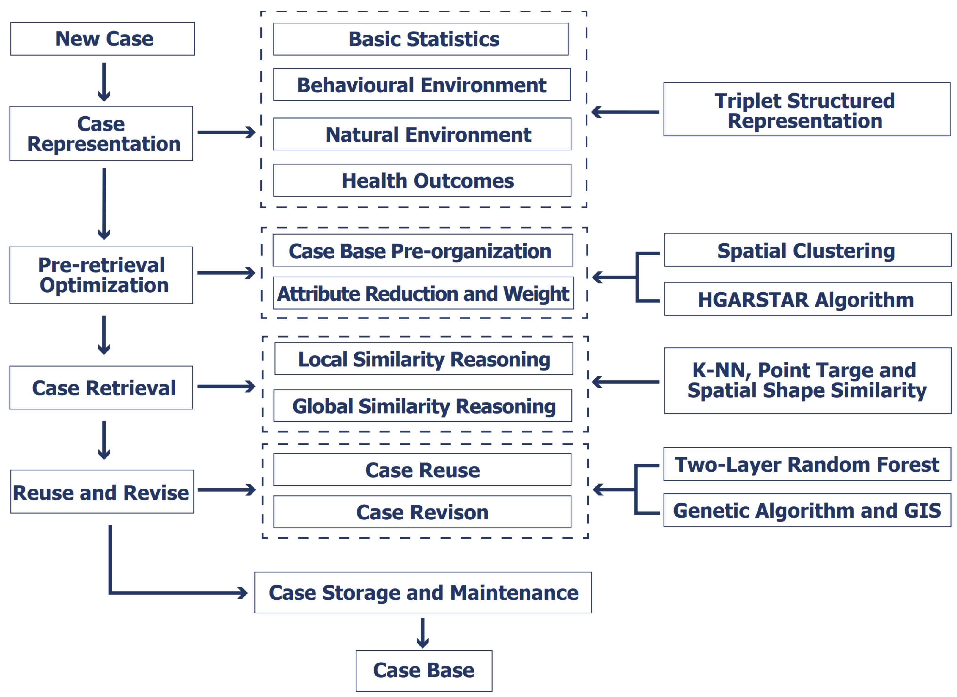
The use of case-based reasoning (CBR) for the assessment of healthy cities necessitates the consideration of the representation of historical cases, the retrieval of similar cases, and the reuse and revision of cases, reflecting the logical and creative thought processes of the CBR model. To enhance the precision, robustness, and efficiency of CBR, we propose the Health City Spatial Case-Based Reasoning (HCSCBR) model. This model incorporates spatial geographic features in the assessment of healthy cities, pre-organizes cases, reduces attributes, assigns weights prior to case retrieval, and considers multiple spatial driving factors. Our research is divided into four stages: (a) representation of cases with spatial features; (b) pre-organization of the case library, attribute reduction, and weight allocation for retrieval optimization before case retrieval; (c) case retrieval considering both global and local similarity inferences; and (d) case reuse and revision. The proposed HCSCBR framework is illustrated in Figure 1.
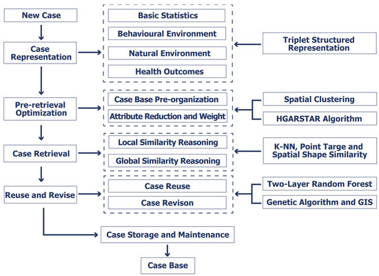
Figure 1.
Research Framework of HCSCBR.
2.2. Establishment of a Case Database
To retrieve similar cases using the HCSCBR method, we have established a case database, which serves as the foundational unit of case-based reasoning. The content and structure of the case database are critical factors influencing the success of case reasoning.
2.2.1. Data Sources
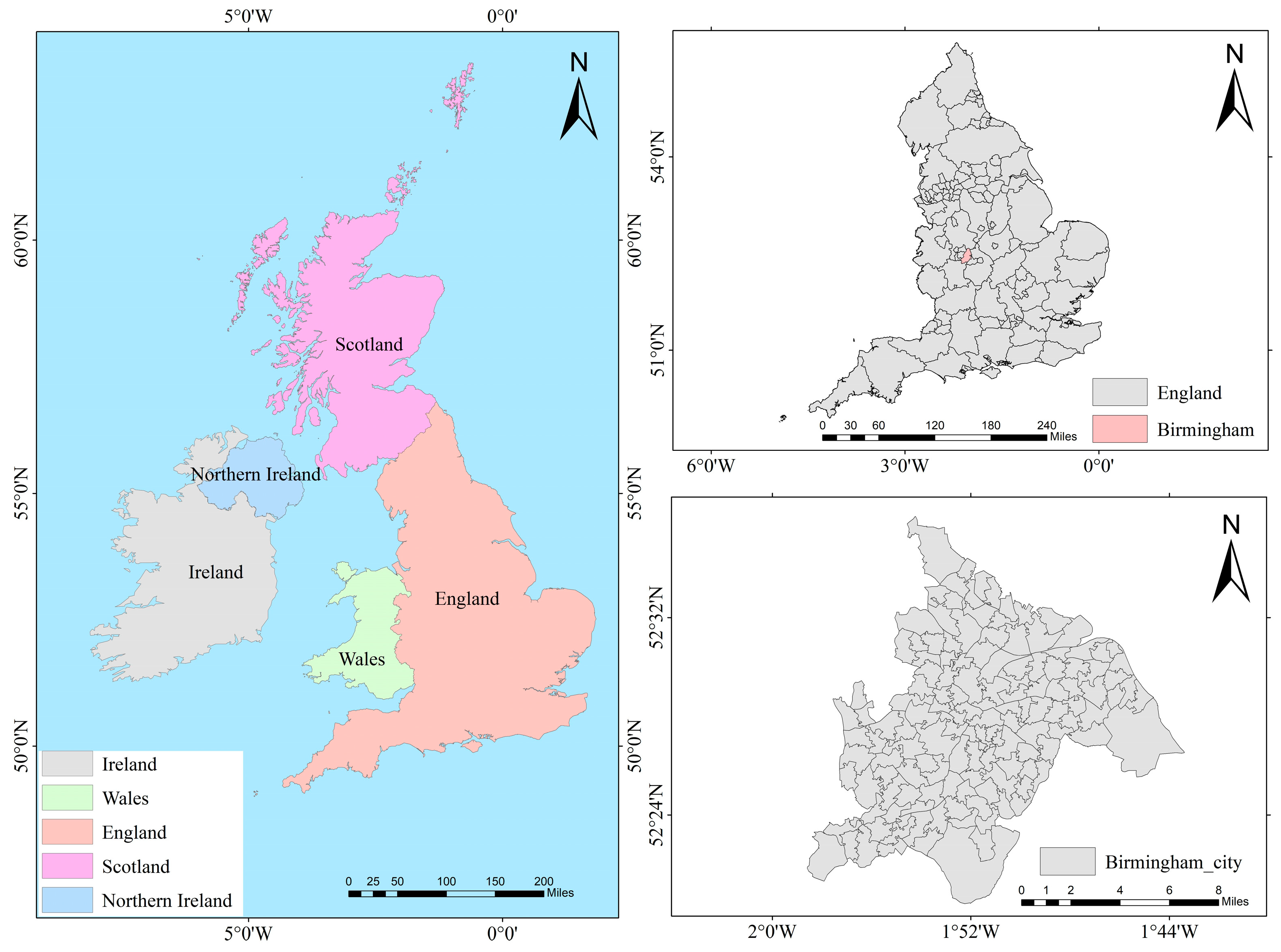
The evaluation of healthy cities is a comprehensive assessment involving multiple dimensions, levels, and stakeholders. It requires consideration of factors such as environment, economy, society, population, services, and space as well as the expectations and needs of different stakeholders. Therefore, the characteristic attribute variables of the case database should comprehensively reflect the impact factors and behavioral factors affecting the health status of cities. However, due to regional differences in the assessment of healthy cities, data formats are often messy, spatial resolutions vary, and it is challenging to unify multi-source heterogeneous data at the same spatial scale. There is a need to bridge the data gap between urban environments and citizens’ health outcomes, as well as the social gap between data sources and researchers. To ensure the rationality and validity of the data, this study uses a fine-grained health dataset of health environmental determinants provided by the literature [24], which integrates different data sources into two unified spatial scales: middle-layer super output areas (MSOAs) and the city level. This dataset covers 1039 MSOAs in 29 cities in England, with a time range from 2019 to 2022 (Figure 2).
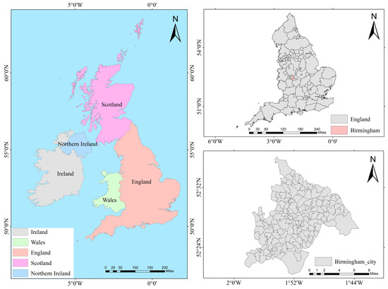
Figure 2.
Birmingham, England’s 135 MSOAs.
The dataset consists of two major parts: citizens’ health outcomes and the corresponding environmental determinants. Specifically, health outcome data reflect the expected lifespan, physical health, and mental health of each region. Basic statistical data, including the population, area, boundaries, and centroid of the selected areas, provide necessary information to understand the spatial composition of cities. Behavioral environment data, such as the availability of tobacco, alcohol, physical exercise, and healthcare services in communities, are considered important health-related behavioral factors, gathered through point of interest (POI) data. The built environment of a city, a significant determinant of health, influences the physical activities and mental health of citizens; architectural density, road network density, street view features, satellite features, and walkability together describe the built environment of urban space. Exposure to polluted air and climate issues have always been seen as major health challenges. Natural environmental data mainly include daily average records of nitrogen oxides such as nitrogen dioxide, PM2.5, and PM10 particles, serving as air pollution indicators in our dataset. Temperature, precipitation, relative humidity, sunshine duration, snow days, and wind speed serve as weather characteristic indicators. All data have been quantitatively described and are openly available through the GitHub repository [24].
2.2.2. Spatial Case Representation
Case representation is a collection of features and attributes that directly affects the precision and efficiency of case-based reasoning. Unlike traditional CBR, which focuses primarily on attribute features, HCSCBR considers both attributes and spatial features. Spatial features enhance the accuracy and efficiency of case retrieval and reuse, addressing complex, heterogeneous geographic problems.
Our applied case structure model is a top-level design for application cases, developed after extensive abstraction. Each middle-layer super output area (MSOA) serves as an evaluation unit. This case representation includes attribute features related to physical health, mental health, life expectancy, basic statistics, behavioral environment, built environment, and natural environment. Among these attributes, boundary data and centroid data represent information at different spatial scales, articulating geographic boundaries for each MSOA or city, and highlighting spatial distribution and regional differences. Geographic spatial features are fully integrated into the regional health risk assessment model, with boundary data and centroid data chosen as spatial features. For city-level case representation, data from MSOA levels are aggregated following city boundaries, supporting health assessments on a city scale.
To effectively describe healthy city evaluation cases, we abstract the cases into a tripartite representation based on the regional differentiation characteristics of the geographic space where the geoscience problem is located. This representation includes three parts: “problem space”, “environment space”, and “solution space”. The “problem space” primarily comprises basic statistical data, natural environment indicators, and behavioral environment indicators. The “environment space” quantitatively expresses the impact of the built environment on the problem space, incorporating spatial morphology and various attribute features such as road density, street view features, MSOA boundaries, and centroids. The “solution space” encompasses attributes related to citizens’ physical health, mental health, and life expectancy. The mathematical expression for case representation is defined as follows:
Here, k represents the number of source cases, and Ak, Sk, and Rk represent the problem space, environment space, and solution space of the case, respectively.
where ai,k represents the description value of the ith attribute feature in the kth case and j is the number of attribute features. Major attribute features include city environmental determinants, such as population and area attributes in basic statistics; attributes in the behavioral environment like tobacco availability, alcohol availability, health service availability, and physical exercise availability; and attributes in the natural environment, like NOx, PM2.5, PM10, minimum and maximum temperature, rainfall, and relative humidity.
where si,k represents the description value of the ith spatial feature attribute in the kth case and l is the number of spatial relation attributes. Spatial attribute features include the MSOA boundary and centroid data in the built environment.
where ri,k represents the description value of the ith result attribute in the kth case and m is the number of result attributes. Outcome attributes include physical health attributes such as the number of confirmed COVID-19 cases, asthma medication expenditure, and obesity rates, as well as mental health attributes such as mental health medication expenditure and mental health services utilization rates.
Ck: <Ak; Sk; R>, k = 1, 2, …, n
Ak = {a1,k, a2,k, …, ai,k, …, aj,k}
Sk = {s1,k, s2,k,…, si,k,…, sl,k}
Rk = {r1,i, r2,i, …, ri,k, …, rm,k}
2.3. Case Pre-Organization
A large number of effective cases ensure the success of case retrieval. However, as the number of cases in the case base increases, and each case has its spatial element, retrieving them consumes a considerable amount of computational resources. If only conventional retrieval and matching algorithms are used, the efficiency of retrieval will be significantly reduced, and it may even be challenging to achieve satisfactory results [39]. In the case of organization and maintenance, many studies have adopted clustering methods and data mining techniques to divide the case base into sub-libraries to improve retrieval efficiency [39,40,41,42]. Although these traditional clustering algorithms meet some specific applications, they still have various degrees of shortcomings, such as the need for prior knowledge and preset parameters, inability to discover clusters of arbitrary shapes, difficulty in dealing with clusters of varying internal density, and issues with outliers and noise [43].
According to Tobler’s First Law of Geography [44], “entities that are closer in space are more similar than those that are further apart”. If the distance between two points is sufficiently small, they are considered to be similar points. Therefore, before case retrieval, it is possible to perform spatial clustering on the centroids of MSOAs to pre-organize cases, thereby forming highly similar sub-cases to optimize retrieval efficiency and localization accuracy.
We adopt an adaptive spatial clustering algorithm based on Gestalt theory and scanning circle technology, referred to as ASC [43]. This algorithm is capable of discovering clusters of any shape based on centroids and does not depend on modifying the initial model (such as the minimum spanning tree, Delaunay triangulation, Voronoi diagram, etc.). The algorithm is straightforward to understand and implement, scalable, and not limited by the size of the dataset, achieving good results in clustering tasks.
2.4. Attribute Reduction and Weight Assignment
Attribute reduction and weight assignment involve identifying representative features and their weights, eliminating redundant features, and exploring decisive key factors and weights. These processes are crucial for improving the accuracy and efficiency of case-based reasoning (CBR) matching [45]. Rough set theory (RST) has proven to be an effective tool for subset selection of features. The rough set algorithm can handle some indiscernible phenomena using incomplete information or knowledge. By reflecting the inaccuracy and uncertainty of the objective world, it can mine the patterns implied in the data without relying on expert knowledge, ensuring objectivity in determining the weights of evaluation factors. Additionally, it can find the minimum data set through data reduction, assess the value of data, and provide a clear and easy-to-understand explanation of the results. Thus, it is widely used in feature selection and weight determination [38,40,46].
As the size of the case base increases and the significant non-spatial attribute features multiply, the complexity of using rough set reduction and weight assignment directly increases exponentially. Meanwhile, genetic algorithms can globally optimize the problem with advantages like implicit parallelism. Therefore, given the characteristics of large data volumes and high attribute redundancy in the case base, this study adopts an HGARSTAR algorithm that combines rough set and genetic algorithms for feature extraction [47], used for case attribute reduction. The HGARSTAR algorithm embeds a local search operation of rough sets to enhance the reinforcement capability of the genetic algorithm. All candidate objects generated during the evolutionary process are forced to include core features to accelerate convergence. Various reduced features have different importances. According to the definition and dependency degree of rough sets, the weights of various indicators in the decision table can be constructed. For example, in the information system —where —the importance of condition , , is given by:
Therefore, the weight of is:
2.5. Integrated Reasoning of Attribute and Spatial Similarity
In the CBR cycle, case retrieval is the most crucial step as it usually determines the performance of the CBR system [48]. Traditional CBR reasoning methods include inductive retrieval methods, knowledge-based retrieval methods, and the nearest neighbor algorithm. The Euclidean distance nearest neighbor algorithm (K-NN) is widely used as a case retrieval method [49]. Case retrieval is the core of case reasoning. The health city evaluation case similarity retrieval consists of two parts: attribute similarity calculation and spatial feature similarity calculation. Based on the integrated reasoning of attribute and spatial similarity, the solution of the known case with the highest similarity is taken as the solution of the unknown case.
2.5.1. Calculation of Attribute Feature Similarity
For case retrieval, traditional CBR reasoning methods include inductive retrieval methods, knowledge-based retrieval methods, and the nearest neighbor algorithms. Among these, the nearest neighbor algorithm is widely adopted for case retrieval. This study uses the traditional nearest neighbor method for attribute similarity retrieval [49]. According to the nearest neighbor retrieval method, the attribute similarity between the target case A and the source case B is calculated as:
where is the weight of the ith feature attribute and satisfies:
2.5.2. Calculation of Spatial Feature Similarity
The computation of similarity in geographic spatial data is one of the key techniques in case-based reasoning. The similar spatial characteristics of a geographical space target refer to geometric similarity, such as location and dimension, and similarities in spatial relationships, such as topology, direction, and distance. All these aspects must be included in the calculation of spatial similarity [50]. The evaluation results of healthy cities are easily affected by the adjacent geographical environment, which is manifested in spatial relationship dependencies or constraining relationships among cases. Therefore, in case retrieval, the calculation of the similarity of spatial characteristics must also be considered. In this research, we adopt the distance between the source case and the target case, as well as the similarity in spatial form and size between the source case and the target case for matching calculations.
- Calculation of Similarity for Spatial Point Targets
Suppose that the topology relationship, distance relationship, direction relationship, distribution range, and density are represented by a five-dimensional vector. We can calculate the spatial similarity using the weighted Euclidean distance, which is:
The spatial similarity in the source case is calculated between the city or MSOA centroid (mass point) and the city or MSOA centroid (mass point) in the historical case, where α\alphaα is a positive constant that adjusts the distance, affecting the similarity. is a number between 0 and 1. is their weighted Euclidean distance, defined as:
Here, A and B are three-dimensional vectors representing the spatial features of two points. and are the kth components of vectors A and B, respectively, representing topological relationships, distance relationships, and directional relationships. is the variance or weight of the kth dimension, indicating the degree of influence of that feature on spatial distance.
- 2.
- Calculation of Spatial Relationship Morphology Similarity
The calculation of spatial relationship morphology similarity for MSOAs or cities primarily includes the computation of spatial relationships and geometric features of spatial face group targets. The equation is as follows:
where represents the spatial similarity between spatial forms A and B, is the degree of spatial difference between spatial forms A and B, and and are the self-differences of spatial forms A and B, respectively. The method for calculating spatial difference is as follows:
where n and m are the number of faces in spatial forms A and B, respectively; and are the areas of the ith and jth faces, respectively; and are the weight coefficients for the ith and jth faces, respectively (which can be set according to different objectives); and and are the geometric feature functions for the ith and jth faces, respectively (which can be total area, total perimeter, compactness, face density, etc.). The overall spatial similarity is:
where and are the weights for spatial proximity and spatial form, respectively. and are the similarities of spatial proximity and spatial form between the source case A and the target case B, respectively. is the comprehensive spatial similarity. The weights and are determined according to reference [51].
- 3.
- Comprehensive Similarity
The comprehensive reasoning of attribute and spatial similarity combines Equations (7) and (13) to calculate the overall similarity as follows:
where and are the weight coefficients for attribute similarity reasoning and spatial feature similarity reasoning, respectively. and represent the similarities of attribute features and spatial features, respectively. is the set of similar cases obtained according to a predefined threshold 0.85.
Therefore, the maximum similarity can be obtained as:
2.6. Case Reuse
Considering that the retrieved target cases are seldom identical to the source cases, it is necessary to obtain proposed solutions for the target cases from similar cases with the highest similarity through case reuse. A two-layer random forest model [42] is employed to enhance the accuracy and stability of case reuse. If the highest similarity corresponds to q case records, then the record most similar to the target case Ck is:
where represents the record of the case with the highest similarity, represents the problem description, and represents the proposed solution for the target case. When the proposed solution completely contradicts the actual situation, case revision is required.
2.7. Case Revision
Case revision is a process of modification or update of existing cases during case-based reasoning (CBR), aimed at enhancing the efficiency and accuracy of reasoning. It not only reflects the logical and creative thinking of the CBR model but also presents its challenges and critical aspects [52]. Consequently, an effective case revision method can not only enhance the performance of CBR but also has significant importance for artificial intelligence in addressing actual engineering problems. Currently, manual correction by domain experts and machine learning methods are the primary methods for case revision [53]. In recent years, to overcome the drawbacks of these methods, the academic community has adopted techniques such as genetic algorithms [54], multivariate regression [55], decision groups [56], etc., enhancing the degree of automation in CBR case reuse and revision stages. In health city evaluation, considering the importance of spatial information increases the difficulty of case revision.
Our research adopts the case revision method for spatial similarity and relationships proposed by [20], which includes two steps: case evaluation and case revision. Case evaluation is done by defining the compatibility of similar cases with the target case, computing the degree of conformity for each feature, and identifying the differential characteristics that need revision. Case revision is based on differential characteristics, for non-spatial attributes and spatial attributes. Non-spatial attribute revision employs genetic algorithms, using binary coding, fitness functions, selection, crossover, mutation, and other operations to optimize the solution of similar cases to better meet the requirements of the target case. Spatial attribute revision uses GIS grid mapping technology, leveraging spatial position information to map the geographical environment attributes of similar cases to the corresponding layers or partition layers in the health city spatial database, checking its consistency with the actual situation, and making necessary modifications.
3. Case Study and Results Analysis
3.1. Construction of the Case Base
For the construction of the historic case base in this study, we used data from 1039 MSOAs (middle-layer super output areas) covering 29 cities in England as experimental data, utilizing mathematical expressions in the process of establishing the source case base. The MSOA data span from 2019 to 2022. For computational convenience, we take cross-sectional data averages of median/mean house price, NOx, PM2.5, PM10 indices (μg/m3), lowest/highest temperatures (°C), rainfall (mm), relative humidity (%), snowfall days (days per month), sunlight hours (hours per month), and wind speed (knots) as feature attribute values.
Regarding the four environmental spatial attribute features, involving MSOA centroid points and boundary coordinate spatial proximity, we calculate the spatial proximity among different MSOAs using a spatial weight matrix. The topological relationships of MSOAs are defined and checked through topological rules, such as zones must not overlap, must be adjacent, and borders must match. These can be accomplished using the “Spatial Relationship Analysis” tool in ArcGIS.
The solution space selects the four diseases with higher incidence rates in physical health in England: cancer, dementia, diabetes, and asthma along with mental health and life expectancy, which include mental health, life expectancy, and healthy life expectancy, totaling seven attribute features. For cancer, dementia, diabetes, asthma, and mental health, we use the average of cross-sectional data representing actual medical expenses to measure, as shown in Table 1 for the case base’s attribute features.

Table 1.
Attributes of the Case Library.
3.2. Spatial Clustering Organization of Case Library
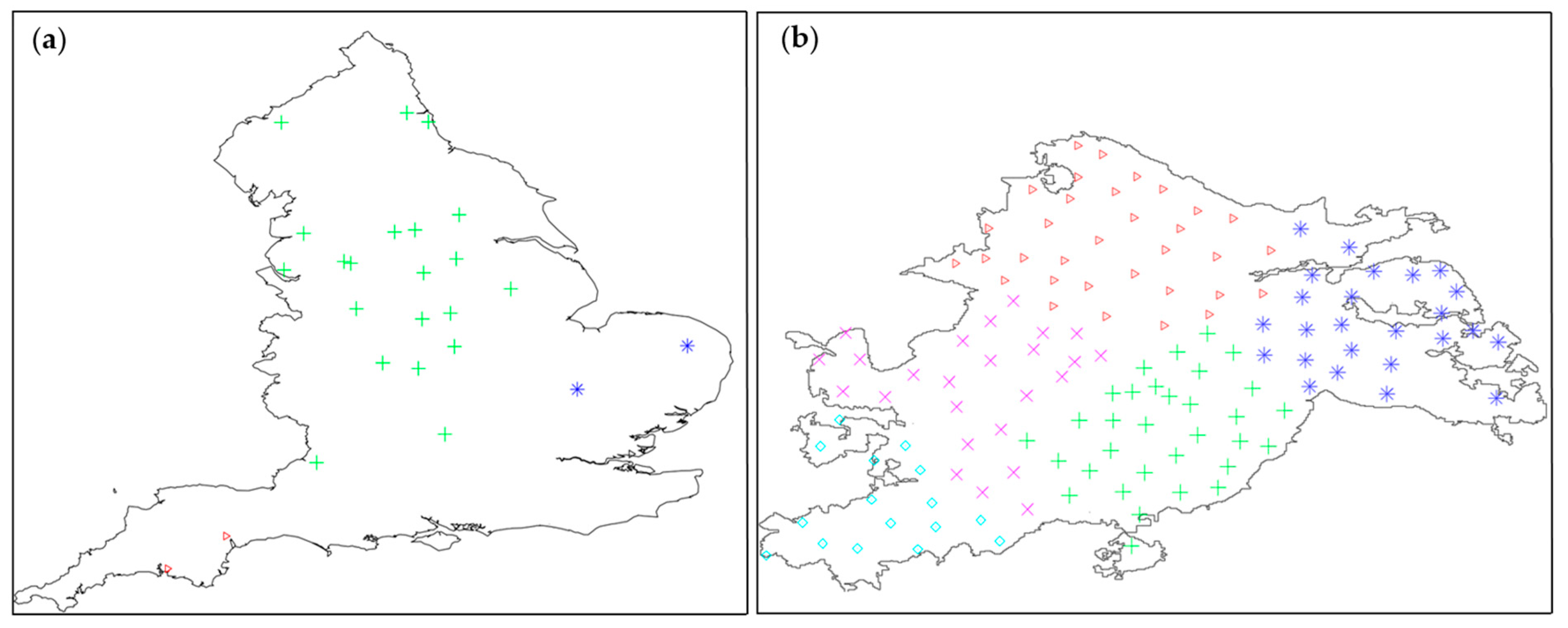
The ASC spatial clustering algorithm, as mentioned in Section 2.3, is used to perform primary spatial clustering on the centroids of the 29 cities, followed by secondary spatial clustering within each city’s MSOAs. As shown in Figure 3, the 29 cities are divided into 3 primary clusters. Within these clusters, for instance, Birmingham’s 135 MSOAs are further divided into five sub-clusters, with each sub-cluster representing a secondary index. During the retrieval of source cases, prioritizing adjacent clusters enhances the precision and efficiency of retrieving target cases. In this process, cases with disorganized spatial positions are considered outliers and are disregarded.
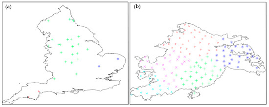
Figure 3.
Pre-organization of the case: (a) 29 cities in England generate 3 clusters; (b) 135 MSOAs in Birmingham generate 5 clusters.
3.3. Feature Extraction and Weight Allocation
Before calculating the feature extraction and weight allocation of attribute data, it is important to consider that case attributes can have different dimensions, which can affect the results of data analysis. To eliminate the impact of these varying dimensions, we need to normalize the data. For the ith attribute value of each case, normalization can be carried out using the following formula:
Here, represents the standardized value, where each feature attribute’s data is uniformly mapped onto an interval. According to the HGARSTAR method [47], the main attribute features and weights are extracted, as shown in Table 2.
Table 2.
Selection of non-spatial feature attributes and weight allocation.
3.4. Case Retrieval and Revision
Case retrieval refers to the method of similarity reasoning according to Formulas (14) and (15), involving the setting of weight coefficients for 16 attribute feature variables based on the experimental results in Table 2. For the weights of spatial relationship morphology similarity calculations in Formulas (11)–(13), since there are fewer feature factors involved in spatial morphology similarity calculations, the weights are assigned a 1:1 value. In Formula (14), and are the weight coefficients for attribute features and spatial features, respectively. Based on their importance, and referring to the literature [38], the sum of the weight coefficients for each attribute feature and spatial feature is obtained as = 0.6859, = 0.3141. The maximum target case similarity is obtained from Formula (15), and the suggested solution is derived according to the same formula. This study adopts the spatial similarity and case revision method for spatial relationships from the literature [20], involving parameter settings in the genetic algorithm. The recommended values according to the literature [47] are shown in Table 3.
Table 3.
Parameter settings in genetic algorithm.
3.5. Experiment and Result Analysis
To validate the effectiveness and practicality of the proposed method in this paper, two experiments, Experiment One and Experiment Two, were designed using the case-based cross-validation method (a 10-fold cross-validation) as described by [57]. The approach involves dividing 1039 historical cases into 10 different groups of samples, labeled 1–10. Of these, 1 group is taken as the test cases, and the other 9 groups are used as source cases; 10 similar cross-validation checks are carried out, respectively. Experiment Three is an application in the real world. To meet the experimental requirements, all the above experiments were carried out on the Windows 11 operating system using Python implementations based on open-source libraries such as NumPy, pandas, SciPy, sklearn, and Keras. The hardware environment used is as follows: CPU is 13th Gen Intel(R) Core(TM) i7-13700 with a frequency of 2.10 GHz, and the RAM is 32.0 GB.
3.5.1. Experiment One: Comparison with Traditional Evaluation Methods
To test the accuracy of this study compared with traditional data mining evaluations, the HCSCBR method proposed in this study was used. We selected methods such as support vector machine (SVM), traditional KNN method, Bayesian network (BN), and artificial neural network (ANN) for comparison. Table 4 shows the comparison results.
Table 4.
Comparison of accuracy with different data mining methods.
The results of the 10 experiments show that, compared with conventional data mining methods, the mean values of evaluation accuracy are as follows: SVM at 87.09%, KNN at 65.69%, BN at 77.90%, and ANN at 74.39%. The accuracy of HCSCBR is the highest, reaching 90.52%. This demonstrates that the proposed algorithm significantly enhances the accuracy of health city evaluations, outperforming other traditional data mining methods.
3.5.2. Experiment Two: Comparison with Other Case-Based Reasoning Methods
To verify the performance of the HCSCBR model proposed in this study in terms of accuracy and effectiveness, we selected the traditional CBR model, which does not consider spatial features, retrieval optimization, or case revision. Given the limited application of CBR in health city research, we selected the model from the literature [38], referred to as SCBR, which also employs the “case question-case attribute-case result” triplet and introduces geographical characteristics. Case retrieval and case modification (reuse) are core parts of case-based reasoning (CBR). The Hybrid_CBR (HCBR) model proposed in the literature [39] not only considers the adoption of fuzzy c-means clustering (FCM) and mutual information to optimize weights for higher retrieval efficiency, but it also establishes an optic regression model for case modification. Therefore, we selected these models for experimental comparison to establish specificity. Given that we introduced clustering analysis to improve CBR performance, the efficiency of CBR is influenced as the case base grows. This experiment compares relative error rate and runtime efficiency, with the expression for the relative error rate being as follows:
where Actval represents the test case, Preval represents the retrieved case, and RER represents the relative error rate. The actual calculation results are shown in Table 5.
Table 5.
Comparison of different CBR methods.
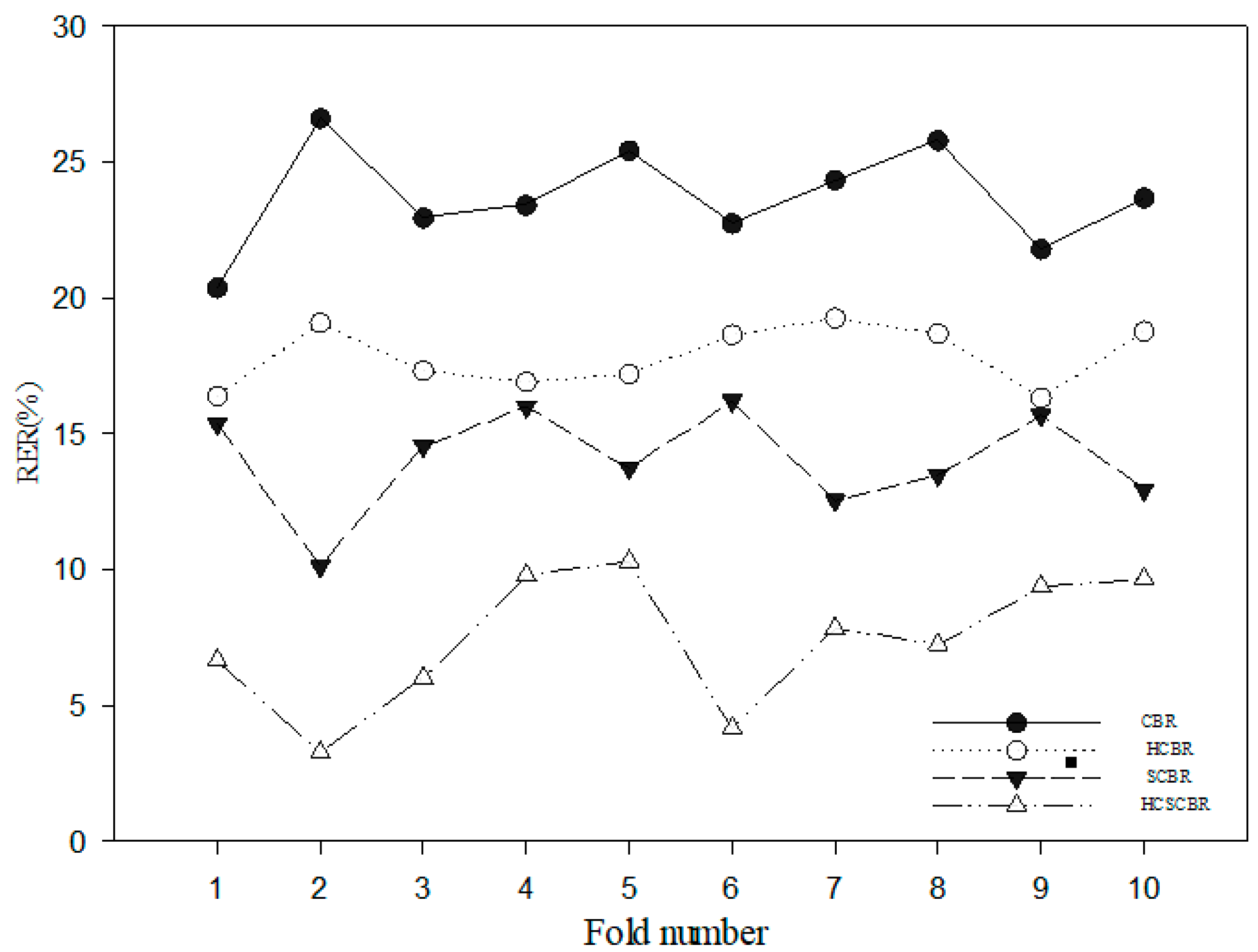
The experimental data in Table 5 show that in the 10 tests, the relative error rate of the HCSCBR model was the lowest at 7.43%, followed by the SCBR model at 14.06%. The error rates of the CBR and HCBR models were relatively high, reaching 23.71% and 17.86%, respectively. This significant lead in error rate is mainly because the CBR and HCBR models do not consider the role of spatial factors in case-based reasoning, which can easily lead to a high error rate. Although both SCBR and HCSCBR are spatial case-based reasoning models, the error rate of the HCSCBR model, which has been spatially corrected, is much lower than that of the SCBR model, which has not been corrected. This difference further emphasizes the importance of case modification in spatial case-based reasoning. Figure 4 shows the comparison results of error rates of different methods in a more intuitive form.
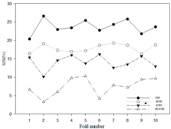
Figure 4.
Error comparison of different CBR methods through 10-fold cross-validation.
In terms of time efficiency, the CBR and HCBR models outperformed the HCSCBR model, with processing times of 0.2428 s and 0.4262 s, respectively, compared to the HCSCBR’s 0.5674 s and SCBR’s 0.6600 s. This indicates that models that do not involve spatial case-based reasoning are relatively more efficient in terms of processing time. However, the HCSCBR model not only uses genetic algorithms and rough set algorithms for weight reduction, but it also divides cases into sub-cases and eliminates noise cases in advance, effectively improving the accuracy and efficiency of retrieval. Compared to the adaptive spatial clustering method used by the SCBR model, although it sacrifices some time efficiency to improve accuracy by adopting case revision methods, the HCSCBR model can still meet the requirements of practical applications overall.
3.5.3. Experiment Three: Real-World Application
This experiment utilized a real set of MSOAs as the target case T to be solved. Case T includes multiple attributes and their corresponding data values, specifically: Population (A1)—7325, Area (A2)—1.52, Population Density (A3)—3729, Geographical Centroid (S1)—(−87.595030, 41.709360), Boundary (S2)—(−86.485210, 41.707250, −86.48679, 41.709340, …), Tobacco Availability (A4)—0.000532, Alcohol Availability (A5)—0.00189, Health Service Availability (A6)—0.00432, Physical Exercise Availability (A7)—0.000635, Building Density (A8)—803, Median/Mean House Price (A9)—172600/192312, Driving/Cycling/Walking Road Density (A10)—15.4/17.2/35.6, Street View Features (A11)—0.0752/0.0429/…, Satellite View Features (A12): 0.138/0.0564/…, Walkability (A13)—0.314, NOx/PM2.5/PM10 (A14)—37/8/11, Min/Max Temperature (A15)—2.5/35, Rainfall (A16)—0.0324, Relative Humidity (A17)—78.3, Snow Lying Days (A18)—7.2, Sunshine Hours (A19)—56.4, Wind Speed (A20)—4.80. Geographical Centroid and Boundary are provided in WGS84 format.
After performing attribute reduction and standardization, the method proposed in this study was used for similarity reasoning. The similarity of variables within each historical case to the new case was calculated. Setting the retrieval threshold to 0.85, the similarity of problem space and solution space for five historical cases is presented in Table 6.
Table 6.
Similarity between retrieval problem attributes and solution attributes.
Before case revision, the primary step involves the evaluation of problem attributes. The value range for feature k in target element T, such as k(A3), k(A4), k(A5), …, k(S2), can be set to Vj (0.75, 1). Accordingly, for the retrieved similar case set , the satisfaction problem evaluation P calculates the compatibility k(P) of each similar case. Table 7 indicates that all retrieved case sets are incompatible with target T, such as case C1, which differs from the target problem with difference features at k(A8), k(A12). Similarly, case C2 has difference features at k(A4), k(A13) with the target problem, and C3,C4,C5 have difference features corresponding to the bold, highlighted numbers in the problem space in Table 7. Therefore, it is necessary to apply the revision method proposed in this research to optimize the solution of the above five similar cases.
Table 7.
Evaluation results of similar cases.
During the process of case revision, we first normalize the similar case set and consider its solutions as the initial population M. Following the recommendations by Jing (2014) [47], we set values for the crossover probability Pc, mutation probability Pm, and the termination number of generations T, as detailed in Table 3. We use MATLAB to solve the genetic algorithm, storing the optimal individual of each generation. Finally, we decode the stable individuals to obtain the solution values: R1 (Asthma)—13,215.08544, R2 (Cancer)—121.31286, R3 (Dementia)—101.54656, R4 (Diabetes)—104.118744, R5 (Mental Health)—6359.91314, R6 (Life Expectancy)—80.3, R7 (Healthy Life Expectancy)—65.7. The solution results match with reality. For spatial geometric feature attributes, such as the MSOA center position, area, etc., we use ArcGIS 10.4 software’s spatial analysis and management module to map and adjust the corresponding spatial attributes.
3.6. Discussion Summary
The innovative HCSCBR model demonstrates significant advantages and potential in healthy city assessments. By incorporating spatial relationships, it addresses the spatial heterogeneity within cities, enhancing evaluation accuracy, especially for spatially dependent health issues. The model’s comprehensive consideration of both attribute and geographic spatial features improves overall performance. Optimization through ASC spatial clustering, genetic algorithms, and rough set algorithms enhances time efficiency and ensures stability with large datasets. Experimental comparisons show that the HCSCBR model outperforms traditional CBR and other data mining methods in both accuracy and efficiency. Practical applications validate its wide applicability across various health assessment scenarios, from community to city levels, providing valuable support for public health research and urban planning. The successful application of the HCSCBR model highlights its ability to significantly improve the precision and efficiency of healthy city evaluations by integrating spatial relationships and attribute features.
4. Conclusions
In the field of evaluating healthy cities, this paper presented a novel model based on case-based reasoning (CBR) theory, ingeniously integrating spatial relationships, attribute features, and machine learning methods aimed at improving the predictive accuracy of urban health assessments. Through experimental comparisons, we have drawn several important conclusions and findings:
Spatial Relationship Case Reasoning Method: The study successfully developed a case reasoning method incorporating spatial relations, effectively addressing the issue of quantitative assessment in healthy cities. By utilizing spatial relations, this method aligns more closely with the complexity and multidimensionality of actual geographic data.
Consideration of Spatial Features: During the reasoning process, special emphasis was placed on the spatial characteristics of geographical events. This novel perspective not only enhances the stability and adaptability of the CBR model but also delves deep into the intrinsic connections of geographic data, enhancing the model’s comprehensive evaluation capabilities.
Case Pre-organization and Attribute Reduction Algorithm: Through the employment of spatial clustering algorithms, genetic algorithms, and rough set algorithms for case pre-organization and attribute reduction before case retrieval, the time efficiency of spatial case reasoning was significantly enhanced. Such algorithmic design not only optimized the data processing workflow but also ensured the efficiency of the model in handling large-scale data.
Multi-level Evaluation System: The model is not only applicable to the fine-grained MSOA level health assessments but can also aggregate to the city level, forming a comprehensive urban health evaluation system. This provides a more comprehensive and flexible evaluation scale for healthy city assessments.
Future work will focus on incorporating the time dimension to further expand and refine the healthy city evaluation model, enhancing its dynamism and predictive accuracy. Additionally, considering the need for pre-setting parameters when using genetic algorithms, optimizing parameter settings is crucial for improving inference accuracy and efficiency. Further studies will concentrate on exploring more suitable parameter setting methods to fully mine and utilize data characteristics, achieving more accurate and practical healthy city evaluations.
Author Contributions
Shuguang Deng conceived and designed the experiments; Wei Liu performed the experiments; Shuguang Deng, Wei Liu, Ying Peng and Binglin Liu analyzed the data; Shuguang Deng and Wei Liu wrote the paper. All authors have read and agreed to the published version of the manuscript.
Funding
This research was funded by the General Project of Humanities and Social Sciences Research of the Ministry of Education in 2020 (No. 20YJA630011) and the Natural Resources Digital Industry Academy Construction Project.
Data Availability Statement
Data are contained within the article.
Conflicts of Interest
The authors declare no conflicts of interest.
References
- Simos, J.; Spanswick, L.; Palmer, N.; Christie, D. The role of health impact assessment in Phase V of the Healthy Cities European Network. Health Promot. Int. 2015, 30 (Suppl. S1), i71–i85. [Google Scholar] [CrossRef] [PubMed]
- Yang, C.; Tan, S.; Li, M.; Dong, M. Research on active planning intervention strategies for healthy cities. Urban Plan. 2022, 46, 61–76. (In Chinese) [Google Scholar]
- Bai, Y.; Zhang, Y.; Zotova, O.; Pineo, H.; Siri, J.; Liang, L.; Luo, X.; Kwan, M.-P.; Ji, J.; Jiang, X.; et al. Healthy cities initiative in China: Progress, challenges, and the way forward. Lancet Reg. Health-West. Pac. 2022, 27, 100539. [Google Scholar] [CrossRef]
- Zhao, M.; Qin, W.; Zhang, S.; Qi, F.; Li, X.; Lan, X. Assessing the construction of a Healthy City in China: A conceptual framework and evaluation index system. Public Health 2023, 220, 88–95. [Google Scholar] [CrossRef] [PubMed]
- Boeing, G.; Higgs, C.; Liu, S.; Giles-Corti, B.; Sallis, J.F.; Cerin, E.; Lowe, M.; Adlakha, D.; Hinckson, E.; Moudon, A.V. Using Open Data and Open-Source Software to Develop Spatial Indicators of Urban Design and Transport Features for Achieving Healthy and Sustainable Cities. Lancet Glob. Health 2022, 10, e907–e918. [Google Scholar] [CrossRef] [PubMed]
- Lowe, M.; Arundel, J.; Hooper, P.; Rozek, J.; Higgs, C.; Roberts, R.; Giles-Corti, B. Liveability aspirations and realities: Implementation of urban policies designed to create healthy cities in Australia. Soc. Sci. Med. 2020, 245, 112713. [Google Scholar] [CrossRef]
- Forsyth, A.; Slotterback, C.S.; Krizek, K.J. Health impact assessment in planning: Development of the design for health HIA tools. Environ. Impact Assess. Rev. 2010, 30, 42–51. [Google Scholar] [CrossRef]
- Sharma, M.; Netherton, A.; McLarty, K.; Petrokofsky, C.; Chang, M. Professional workforce training needs for Health Impact Assessment in spatial planning: A cross sectional survey. Public Health Pract. 2022, 3, 100268. [Google Scholar] [CrossRef] [PubMed]
- Luo, J.; Chan, E.H.W.; Du, J.; Feng, L.; Jiang, P.; Xu, Y. Developing a Health-Spatial Indicator System for a Healthy City in Small and Midsized Cities. Int. J. Environ. Res. Public Health 2022, 19, 3294. [Google Scholar] [CrossRef]
- Orsetti, E.; Tollin, N.; Lehmann, M.; Valderrama, V.A.; Morató, J. Building Resilient Cities: Climate Change and Health Interlinkages in the Planning of Public Spaces. Int. J. Environ. Res. Public Health 2022, 19, 1355. [Google Scholar] [CrossRef]
- Wu, S.; Li, D.; Wang, X.; Li, S. Examining component-based city health by implementing a fuzzy evaluation approach. Ecol. Indic. 2018, 93, 791–803. [Google Scholar] [CrossRef]
- Gong, X.; Liu, J.; Wu, L.; Bu, Z.; Zhu, Z. Development of a Healthy Assessment System for Residential Building Epidemic Prevention. Build. Environ. 2021, 202, 108038. [Google Scholar] [CrossRef] [PubMed]
- de Leeuw, E.; Green, G.; Dyakova, M.; Spanswick, L.; Palmer, N. European Healthy Cities evaluation: Conceptual framework and methodology. Health Promot. Int. 2015, 30 (Suppl. S1), i8–i17. [Google Scholar] [CrossRef] [PubMed]
- Abe, K.C.; Rodrigues, M.A.; Miraglia, S.G.E.K. Health impact assessment of air pollution in Lisbon, Portugal. J. Air Waste Manag. Assoc. 2022, 72, 1307–1315. [Google Scholar] [CrossRef] [PubMed]
- Hua, J.; Zhang, X.; Ren, C.; Shi, Y.; Lee, T.-C. Spatiotemporal assessment of extreme heat risk for high-density cities: A case study of Hong Kong from 2006 to 2016. Sustain. Cities Soc. 2021, 64, 102507. [Google Scholar] [CrossRef]
- Li, S.; Zhang, J.; Moriyama, M.; Kazawa, K. Spatially heterogeneous associations between the built environment and objective health outcomes in Japanese cities. Int. J. Environ. Health Res. 2022, 33, 1205–1217. [Google Scholar] [CrossRef] [PubMed]
- Iungman, T.; Cirach, M.; Marando, F.; Pereira Barboza, E.; Khomenko, S.; Masselot, P.; Quijal-Zamorano, M.; Mueller, N.; Gasparrini, A.; Urquiza, J.; et al. Cooling cities through urban green infrastructure: A health impact assessment of European cities. Lancet 2023, 401, 577–589. [Google Scholar] [CrossRef] [PubMed]
- Pala, D.; Caldarone, A.A.; Franzini, M.; Malovini, A.; Larizza, C.; Casella, V.; Bellazzi, R. Deep Learning to Unveil Correlations between Urban Landscape and Population Health. Sensors 2020, 20, 2105. [Google Scholar] [CrossRef] [PubMed]
- Elbaz, K.; Hoteit, I.; Shaban, W.M.; Shen, S.-L. Spatiotemporal air quality forecasting and health risk assessment over smart city of NEOM. Chemosphere 2023, 313, 137636. [Google Scholar] [CrossRef]
- Deng, S.; Li, W. Spatial case revision in case-based reasoning for risk assessment of geological disasters. Geomat. Nat. Hazards Risk 2020, 11, 1052–1074. [Google Scholar] [CrossRef]
- Merghadi, A.; Yunus, A.P.; Dou, J.; Whiteley, J.; Thaipham, B.; Bui, D.T.; Avtar, R.; Abderrahmane, B. Machine learning methods for landslide susceptibility studies: A comparative overview of algorithm performance. Earth Sci. Rev. 2020, 207, 103225. [Google Scholar] [CrossRef]
- Ran, L.; Tan, X.; Xu, Y.; Zhang, K.; Chen, X.; Zhang, Y.; Li, M.; Zhang, Y. The application of subjective and objective method in the evaluation of healthy cities: A case study in Central China. Sustain. Cities Soc. 2021, 65, 102581. [Google Scholar] [CrossRef]
- Lv, Z.; Guo, H.; Zhang, L.; Liang, D. Comparative Study on the Evaluation of Healthy City Construction in Typical Chinese Cities Based on Statistical Data and Land Use Data. Sustainability 2022, 14, 2519. [Google Scholar] [CrossRef]
- Han, Z.; Xia, T.; Xi, Y.; Li, Y. Healthy Cities, A comprehensive dataset for environmental determinants of health in England cities. Sci. Data 2023, 10, 165. [Google Scholar] [CrossRef] [PubMed]
- Jiang, Z.; Jiang, Y.; Wang, Y.; Zhang, H.; Cao, H.; Tian, G. A hybrid approach of rough set and case-based reasoning to remanufacturing process planning. J. Intell. Manuf. 2019, 30, 19–32. [Google Scholar] [CrossRef]
- Aamodt, A.; Plaza, E. Case-Based Reasoning: Foundational Issues, Methodological Variations, and System Approaches. Ai Commun. 2001, 7, 39–59. [Google Scholar] [CrossRef]
- Kwon, N.; Song, K.; Ahn, Y.; Park, M.; Jang, Y. Maintenance cost prediction for aging residential buildings based on case-based reasoning and genetic algorithm. J. Build. Eng. 2020, 28, 101006. [Google Scholar] [CrossRef]
- Ye, X.; Yu, W.W.; Yu, W.H.; Lv, L.N. Simulating urban growth through case-based reasoning. Eur. J. Remote Sens. 2022, 55, 277–290. [Google Scholar] [CrossRef]
- Ye, X.; Yu, W.H.; Lv, L.N.; Zang, S.Y.; Ni, H.W. An Improved Case-Based Reasoning Model for Simulating Urban Growth. Sustainability 2021, 13, 6146. [Google Scholar] [CrossRef]
- Huang, Z.H.; Fan, H.Q.; Shen, L.Y. Case-based reasoning for selection of the best practices in low-carbon city development. Front. Eng. Manag. 2019, 6, 416–432. [Google Scholar] [CrossRef]
- Anthony Jnr, B. A case-based reasoning recommender system for sustainable smart city development. AI Soc. 2021, 36, 159–183. [Google Scholar] [CrossRef]
- Yeh, A.G.O.; Shi, X. Applying case-based reasoning to urban planning: A new planning-support system tool. Environ. Plan. B-Plan. Des. 1999, 26, 101–115. [Google Scholar] [CrossRef]
- Kwon, O.; Kim, Y.S.; Lee, N.; Jung, Y. When Collective Knowledge Meets Crowd Knowledge in a Smart City: A Prediction Method Combining Open Data Keyword Analysis and Case-Based Reasoning. J. Healthc. Eng. 2018, 2018, 7391793. [Google Scholar] [CrossRef] [PubMed]
- Feng, Y.; Li, X.Y. Improving emergency response to cascading disasters: Applying case-based reasoning towards urban critical infrastructure. Int. J. Disaster Risk Reduct. 2018, 30, 244–256. [Google Scholar] [CrossRef]
- Zhang, Y.; Xu, Y.; Li, J. Study on emergency decision-making method of urban fire based on case-based reasoning under incomplete information. J. Saf. Sci. Technol. 2018, 14, 13–18. [Google Scholar]
- Wang, Y.N.; Liang, Y.Z.; Sun, H.; Yang, Y.F. Emergency Response for COVID-19 Prevention and Control in Urban Rail Transit Based on Case-Based Reasoning Method. Discret. Dyn. Nat. Soc. 2020, 2020, 6689089. [Google Scholar] [CrossRef]
- Zhao, Z.; Chen, J.; Yao, J.; Xu, K.; Liao, Y.; Xie, H.; Gan, X. An improved spatial case-based reasoning considering multiple spatial drivers of geographic events and its application in landslide susceptibility mapping. Catena 2023, 223, 106940. [Google Scholar] [CrossRef]
- Du, Y.; Liang, F.; Sun, Y. Integrating spatial relations into case-based reasoning to solve geographic problems. Knowl.-Based Syst. 2012, 33, 111–123. [Google Scholar] [CrossRef]
- Han, M.; Cao, Z.J. An improved case-based reasoning method and its application in endpoint prediction of basic oxygen furnace. Neurocomputing 2015, 149, 1245–1252. [Google Scholar] [CrossRef]
- Zhu, G.N.; Hu, J.; Qi, J.; Ma, J.; Peng, Y.H. An integrated feature selection and cluster analysis techniques for case-based reasoning. Eng. Appl. Artif. Intell. 2015, 39, 14–22. [Google Scholar] [CrossRef]
- Li, H.; Yu, J.L.; Yu, L.A.; Sun, J. The clustering-based case-based reasoning for imbalanced business failure prediction: A hybrid approach through integrating unsupervised process with supervised process. Int. J. Syst. Sci. 2014, 45, 1225–1241. [Google Scholar] [CrossRef]
- Zhong, S.; Xie, X.; Lin, L. Two-layer random forests model for case reuse in case-based reasoning. Expert Syst. Appl. 2015, 42, 9412–9425. [Google Scholar] [CrossRef]
- Zhan, Q.; Deng, S.; Zheng, Z. An Adaptive Sweep-Circle Spatial Clustering Algorithm Based on Gestalt. Int. J. Geo-Inf. 2017, 6, 272. [Google Scholar] [CrossRef]
- Dearman, W.R. 13—Land and water management: Environmental geology mapping. In Engineering Geological Mapping; Butterworth-Heinemann: Oxford, UK, 1991; pp. 339–357. [Google Scholar]
- Yan, A.; Shao, H.; Guo, Z. Weight optimization for case-based reasoning using membrane computing. Inf. Sci. 2014, 287, 109–120. [Google Scholar] [CrossRef]
- Salamo, M.; Golobardes, E. Analysing Rough Sets weighting methods for Case-Based Reasoning Systems. Intel. Artif. Rev. Iberoam. De Intel. Artif. 2002, 6, 1–9. [Google Scholar] [CrossRef]
- Jing, S.Y. A hybrid genetic algorithm for feature subset selection in rough set theory. Soft Comput. 2014, 18, 1373–1382. [Google Scholar] [CrossRef]
- Bouhana, A.; Fekih, A.; Abed, M.; Chabchoub, H. An integrated case-based reasoning approach for personalized itinerary search in multimodal transportation systems. Transp. Res. Part C Emerg. Technol. 2013, 31, 30–50. [Google Scholar] [CrossRef]
- Cover, T.; Hart, P. Nearest neighbor pattern classification. IEEE Trans. Inf. Theor. 2006, 13, 21–27. [Google Scholar] [CrossRef]
- Liu, T.; Yan, H. Geometry Similarity Assessment Model of Spatial Polygon Groups. Geo-Inf. Sci. 2013, 15, 635–642. [Google Scholar] [CrossRef]
- Gong, M.; Yuan, S.; Chu, Z.; Zhang, S.; Fang, C. Underground Pipeline Data Matching Considering Multiple Spatial Similarities. Acta Geod. Cartogr. Sin. 2015, 44, 1392–1400. [Google Scholar]
- Yan, A.; Wang, D. Trustworthiness evaluation and retrieval-based revision method for case-based reasoning classifiers. Expert Syst. Appl. 2015, 42, 8006–8013. [Google Scholar] [CrossRef]
- Yan, A.; Zhang, K.; Yu, Y.; Wang, P. An attribute difference revision method in case-based reasoning and its application. Eng. Appl. Artif. Intell. 2017, 65, 212–219. [Google Scholar] [CrossRef]
- Mohammed, M.A.; Abd Ghani, M.K.; Arunkumar, N.; Obaid, O.I.; Mostafa, S.A.; Jaber, M.M.; Burhanuddin, M.A.; Matar, B.M.; Abdullatif, S.K.; Ibrahim, D.A. Genetic case-based reasoning for improved mobile phone faults diagnosis. Comput. Electr. Eng. 2018, 71, 212–222. [Google Scholar] [CrossRef]
- Jin, R.; Cho, K.; Hyun, C.; Son, M. MRA-based revised CBR model for cost prediction in the early stage of construction projects. Expert Syst. Appl. 2012, 39, 5214–5222. [Google Scholar] [CrossRef]
- Yan, A.; Wang, W.; Zhang, C.; Zhao, H. A fault prediction method that uses improved case-based reasoning to continuously predict the status of a shaft furnace. Inf. Sci. 2014, 259, 269–281. [Google Scholar] [CrossRef]
- Liu, C.H.; Chen, H.C. A novel CBR system for numeric prediction. Inf. Sci. 2012, 185, 178–190. [Google Scholar] [CrossRef]
Disclaimer/Publisher’s Note: The statements, opinions and data contained in all publications are solely those of the individual author(s) and contributor(s) and not of MDPI and/or the editor(s). MDPI and/or the editor(s) disclaim responsibility for any injury to people or property resulting from any ideas, methods, instructions or products referred to in the content. |
© 2024 by the authors. Licensee MDPI, Basel, Switzerland. This article is an open access article distributed under the terms and conditions of the Creative Commons Attribution (CC BY) license (https://creativecommons.org/licenses/by/4.0/).