Factors Influencing the Efficiency of Demand-Responsive Transport Services in Rural Areas: A GIS-Based Method for Optimising and Evaluating Potential Services

Abstract

Demand-responsive transport (DRT) could be an alternative for extending the accessibility of high-speed rail (HSR) servicing cities in rural environments, where fixed public transport does not provide efficient services. This paper proposes a method to analyse the factors that influence the implementation of DRT systems for inter-urban mobility, connecting and integrating towns in rural areas. Methodologically, a vehicle routing problem analysis in a GIS-based environment is applied to a theoretical case study to evaluate the factors that influence DRT efficiency in different scenarios, considering the specific singularities of this kind of inter-urban long-distance mobility. The results suggest the optimal DRT solutions in these rural contexts to be those that, after adjusting the fleet to specific demands, use low-capacity vehicles, which are much better adapted to the geography of sparsely populated areas. Moreover, in adapting DRT systems to HSR travellers’ needs, windows catering to these needs should incorporate the option of setting the pickup or arrival times. This paper demonstrates that DRT systems could reach significant levels of service in rural areas compared with fixed lines and even private vehicles, especially when evaluating key aspects of the system’s efficiency for its implementation.

1. Introduction: Demand-Responsive Transport as an Option for Mobility in Rural Areas

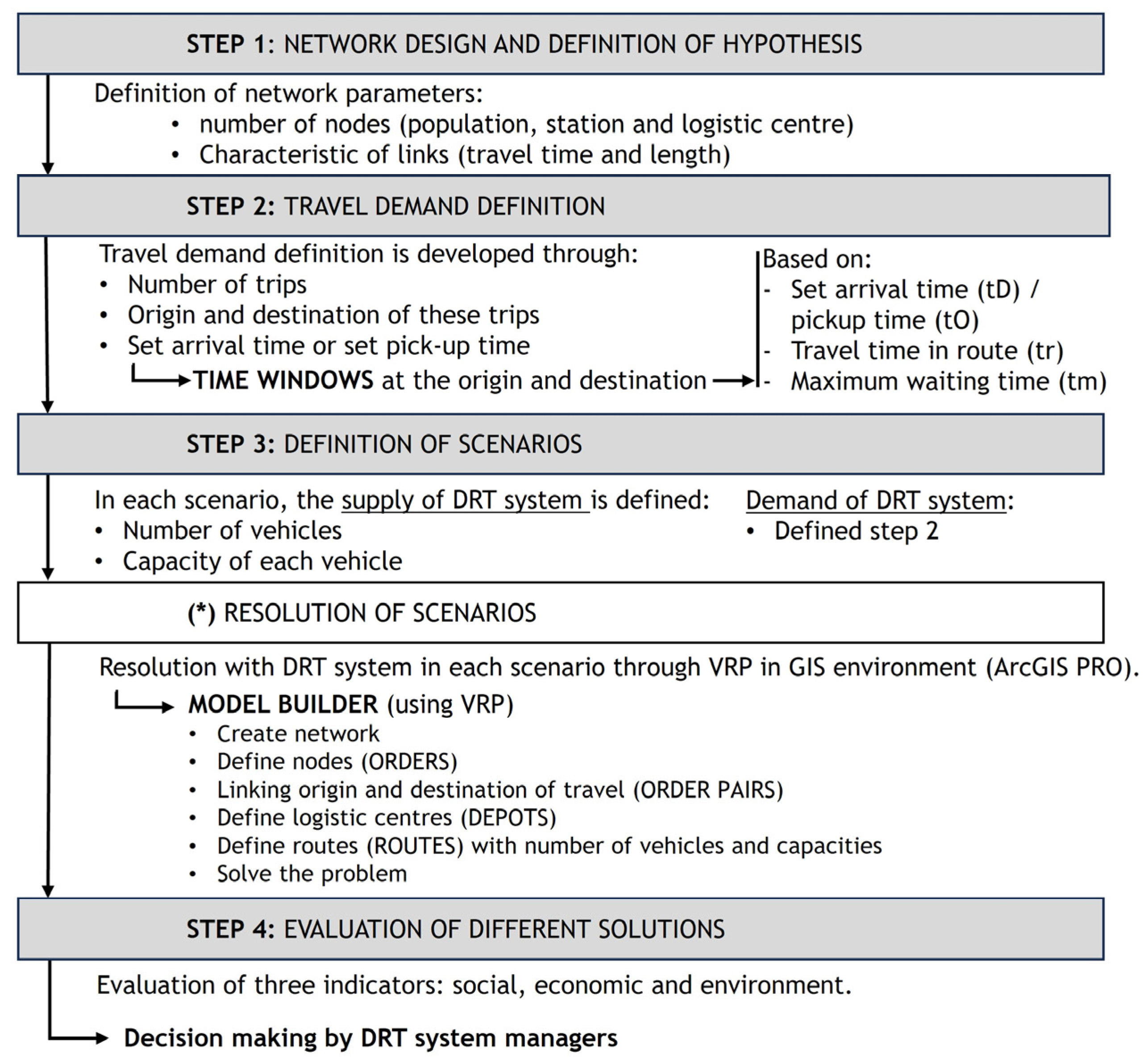
Most rural areas of European countries are experiencing depopulation year after year, mainly because of changing economic activities and a lack of opportunities and services [1,2,3]. In these areas with very low population densities, public transport systems, which are normally implemented and managed with fixed lines of buses, do not usually provide efficient services for the population. The low frequency of such services reduces their usefulness in addressing the specific demands and temporal constraints of travellers. This implies very low accessibility by public transport in rural areas, limiting transport alternatives to private vehicles [4]. In this context, both internationally and locally, there is increasing interest among stakeholders to find more flexible transportation alternatives that could meet the needs of existing mobility demands [5].

In this regard, flexible transport alternatives, such as demand-responsive transport (DRT) systems, could play a fundamental role in improving accessibility in rural areas [6]. DRT systems provide transport services based on users’ demands, using fleets of vehicles and schedules to pick up and drop off in accordance with commuters’ needs [7]. Traditionally, DRT systems have been limited to urban environments and big cities, although it is precisely in rural areas where DRT systems could improve the quality of public transport services as they could adapt better to the needs of individual commuters [8,9], especially in low demand scenarios [10]. However, adapting the services’ characteristics and managing technologies to the singularities of rural environments and the specific needs of the populations living there is absolutely crucial [11].

Although DRT systems are not new (there were some initiatives in the 1960s and 1970s), they have faced technical and economic limitations in recent decades, reducing their expansion and implementation [12,13]. The recent increase in new technologies, such as smartphones, big data sources and faster processing systems, as well as new transportation management approaches, such as ‘Mobility-as-a-Service (MaaS), have opened up new opportunities for this transport alternative. Now, DRT services, combined (or not) with fixed public transport routes, could provide a more flexible and sustainable transport alternative, becoming an ideal solution for improving the accessibility and connectivity of rural areas [14].

These DRT alternatives are not often implemented in rural areas, although there are some references in the literature that consider these geographies. Most of these studies analyse the potential of DRTs as an alternative to fixed lines of public transport in different countries, such as Australia [15], Germany [16,17], Italy [18] and Denmark [19], while others evaluate DRTs as a way of improving the connectivity of suburban and rural areas with railway stations, favouring intermodal connections [20]. Some of these studies also focus on the assessment of some factors for designing DRTs, such as the stop locations and spatial restrictions, or even on potential customer target groups [16]. In this sense, evaluating individual factors that could influence the use and acceptance of DRT in rural areas is key, especially for disabled people and/or pensioners, who are more likely to use this kind of alternative [21]. In summary, although the literature on DRT servicing rural areas is still limited, there is a wide consensus among the studies to date that this flexible transport system could help improve accessibility in rural areas with low population densities due to the flexibility of supply according to users’ demands.

In addition, DRT systems present a challenge in terms of routing optimisation, which needs to be adapted to the demand required and its spatiotemporal daily variations. The existing literature on this topic refers to several methods and algorithms used for routing optimisation. One of the most extended methods is the so-called vehicle routing problem (VRP), which is the problem of designing delivery or pickup routes from one or several depots to several demand orders from different places [22]. Although it was conceived for logistics, the VRP also adapts to the challenge of DRT systems by solving routing problems with pickup and delivery time windows. Several studies have addressed VRP optimisation in their approaches. One of the first examples is the one by Fisher (1993) [23], who studied VRP optimisation using Lagrangian relation approaches to achieve the use of a minimum number of vehicles. Since then, the methods used to solve the VRP have been diverse. On the one hand, some authors have used a state–space–time representation to find the optimal solutions [24], while others have suggested solutions through algorithms that determine high-quality and computationally efficient solutions for on-demand applications [25]. Guo et al. (2019) [26] proposed a mixed integer programming model in which an exact algorithm and two heuristic algorithms were numerically compared. Most of these studies on VRP optimisation have focused on urban areas and have neglected such optimisation in rural areas. Similarly, in the design of DRT systems, the methods and design frameworks presented are mostly adapted to urban environments [27,28]. However, although the models could be applied, DRT systems in rural areas for inter-urban mobility have some characteristics, such as low demand distributed over large areas and longer distances between demand points, which could directly affect DRT systems’ efficiency. Accordingly, these systems need to be carefully analysed before their implementation in these territories.

Another important key factor is the evaluation of DRT performance, since it could help to improve the efficiency of the system’s implementation. The evaluation of DRT is a challenge because of the lack of a common evaluation framework and method in the existing literature. Some studies use evaluation indicators, such as the travel distance, ridership, cost, greenhouse gas emissions and the population’s perception [12], while others propose indicator groups, known as the 5E framework, to analyse the effective mobility, efficient city, economy, environment and quality supports [29] to illustrate the wider benefits of high-quality public transport. Other studies have proposed evaluation frameworks with two-stage bootstrap data envelopment analysis, which combines multiple indicators, and an ordinary least squares method to evaluate a DRT system, reducing the degree of subjectivity to sum up [20]. In addition, the weighting factors of the indicators used depend on each case study [30]. This means that, among the few studies on the subject, there are no unified criteria to be applied.

In summary, most of the studies have focused on optimising and designing DRT in urban areas, and the few examples considering rural environments are generally oriented more towards analysing specific pilot cases and/or users’ perceptions and willingness to adopt DRT services. They usually neglect an analysis of the factors influencing the efficiency of this transport alternative for rural areas, especially the particularities of these territories that could be key to successful implementation. The main objective of this paper is to provide a method to analyse the factors that influence the implementation of DRT systems in rural environments and to identify key aspects in the design of this transportation alternative for inter-urban mobility in dispersed, low-populated rural areas. To achieve this goal, a theoretical case study is proposed to evaluate the different factors and variables that influence the efficiency of a DRT system in different scenarios of supply and demand, considering the specific characteristics of this kind of inter-urban long-distance mobility. Methodologically, a vehicle routing problem analysis integrated in a GIS-based environment is applied to optimise and evaluate the proposed scenarios. An efficient implementation of DRTs adapted to the singularities of rural areas could be key to improving accessibility in these territories, where the efficiency of public transport for inter-urban mobility is not always guaranteed.

2. Methodology

A definition of a DRT system has not been established, and there are many similar concepts based on flexible transport systems. In this research, the DRT concept refers to a flexible transport system with no fixed routes, adapting services to specific user demands and engaging a specific fleet of vehicles to carry passengers [11].

In this research, the main objective is to provide a GIS-based method for the design and implementation of potential DRT systems adapted to inter-urban mobility in rural areas, focusing on an evaluation of the factors influencing the efficiency of the different optimal solutions. For that purpose, we propose a four-step method and apply it to a theoretical case study (Figure 1).

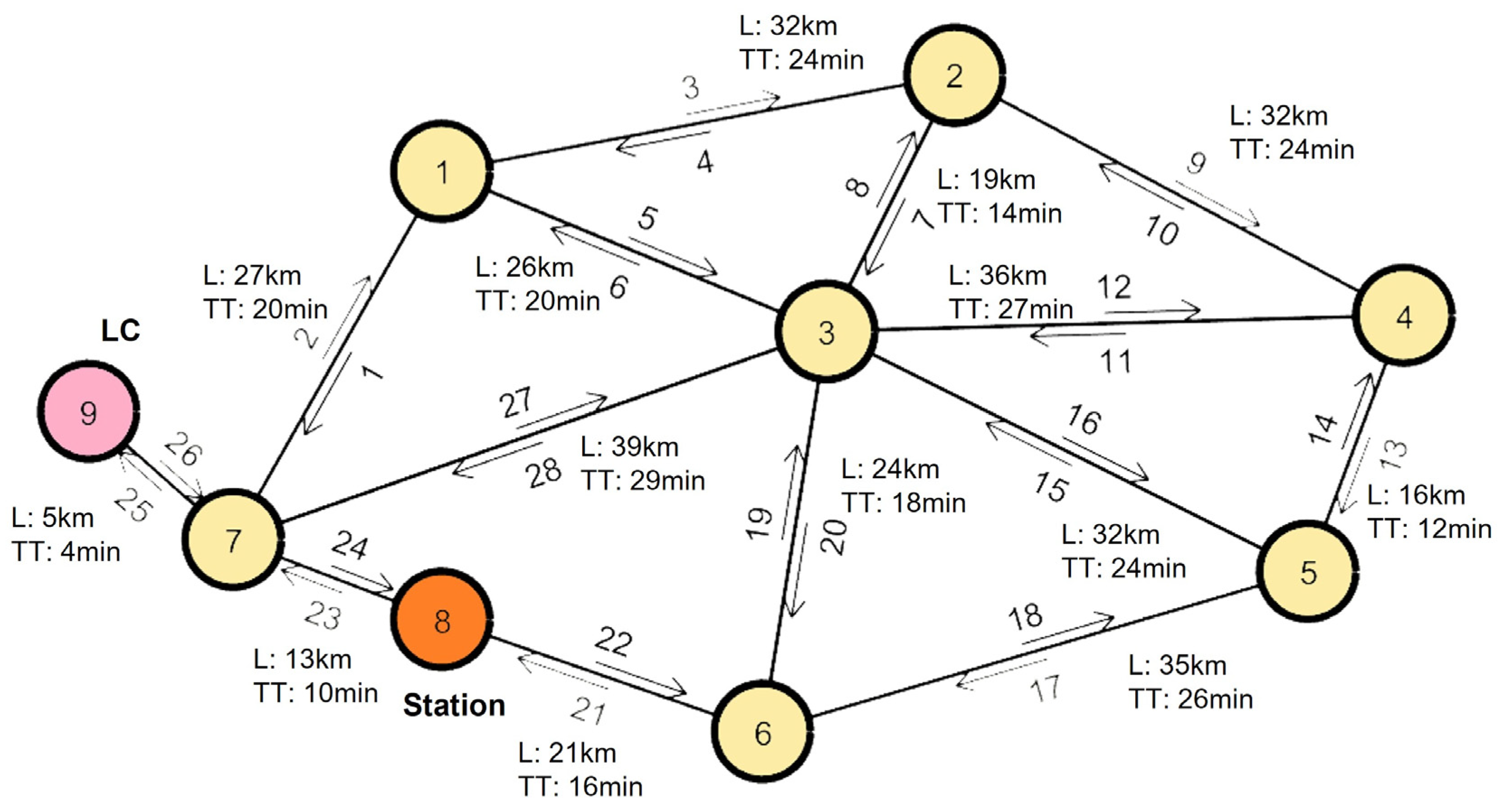
2.1. Step 1: Network Design and Definition of the Hypothesis

The network design for the theoretical case study considered should include the demand points or nodes and road links, with all the elements and parameters involved in the problem. The design and shape adopted in this research are a simplification of the territorial structures in Spain’s low-populated rural areas. These are usually characterised by long distances between towns and cities, which are sometimes served by a railway station located in one of them. Therefore, the theoretical case study proposed is represented using a simplified or ‘toy’ network that includes different nodes, such as population (simulating towns and villages), a logistics centre (LC) for DRT operations and a railway station, which could also be integrated as a node in the network for intermodal long-distance mobility combined with DRTs. Also, the parameters of the links, such as the length (L) and travel time (TT), are defined (Figure 2).

The hypotheses related to the implementation of a DRT system in this toy network are established as follows:

• The transport system is flexible, and the routes of vehicles are defined daily according to users’ demands, considering the pick-up and delivery times of their trips within specific time windows. The start and end points of the routes are both located at the logistics centre.
• DRT services are implemented as static, and travel requests are made one day in advance. In rural areas where transport alternatives are limited and travel demand is low, dynamic routing could be difficult to implement due to population density and the advanced age of the population but also due to longer distances between demand points in different towns. Flexible routes with dynamic routing are more sustainable for moderate demand (20 to 50 requests per square kilometre per hour) [31].

2.2. Step 2: Travel Demand Definition

The travel demands are defined using origin and destination (O-D) matrices, which include the number of passengers per trip requested (this is limited to four passengers to prioritise travel demand over total number of passengers, due to the low population densities in rural areas). The travel requests are defined using time windows that depend, on the one hand, on whether the request is at the origin or destination (green or blue cells, respectively, in

Table 1. Time windows depending on origin–destination requests.

	Origin	Destination
Set arrival time	$\left(t_D-t_m-t_r ; t_D-t_r\right)$	$(t_D-t_m ;{\mathit{t}}_{\mathit{D}})$
Set pick-up time	$({\mathit{t}}_{\mathit{O}} ;t_O+t_m)$	$\left(t_O+t_r ; {(t}_O+t_m)+t_r\right)$

where t_D is the arrival time established/desired by the user, t_O is the pick-up time established/desired by the user, t_r is the travel time of the route, which is calculated by the quickest time by car, and t_m is maximum waiting time the user is willing to wait for the DRT service.

) and, on the other hand, on a maximum waiting time (t_m):

• If the request sets the arrival time at the destination (t_D), then the time window at the destination is set as (t_D − t_m; t_D). To establish the origin time window, the travel time of the shortest route (t_r) is used (the travel time of the route (t_r) is calculated considering the minimum travel time of the route by private car. Therefore, the origin time window is (t_D − t_m − t_r; t_D − t_r).
• If the request sets the departure time at the origin, i.e., the desired pickup time (t_O) at the origin, then, considering the defined maximum waiting time, the time window at the origin is set as (t_O; t_O + t_m). Then, the destination time window is established using the travel time (t_r) of the shortest route. Therefore, the destination time window is (t_O + t_r; t_O + t_m+ t_r).

To analyse several demand levels, different O-D matrices have been simulated with different numbers of trips and maximum waiting times (t_m) (see Section 3.3). In a specific case,

Table 2. Example of the O-D matrix of 12 trips with t_m 30 min.

OD Matrix 12 Trips with Time Windows (tm 30)
	To	POP 1	POP 2	POP 3	POP 4	POP 5	POP 6	POP 7	Station
From
POP 1			0	3 [9.18; 9.48]; [9.30; 10.00]	0	0	0	0	2 [13.00; 13.30]; [13.30; 14.00]
POP 2		0		0	0	0	0	0	1 [12.42; 13.12]; [13.30; 14.00]
POP 3		0	0		0	3 [11.06; 11.36]; [11.30; 12.00]	0	0	0
POP 4		0	0	0		0	2 [11.22; 11.52]; [12.00; 12.30]	0
POP 5		0	0	0	0		0	0	3 [12.48; 13.18]; [13.30; 14.00]
POP 6		0	3 [11.58; 12.28]; [12.30; 13.00]	0	0	0		0	0
POP 7		0	0	1 [10.01; 10.31]; [10.30; 11.00]	0	0	0		4 [14.20; 14.50]; [14.30; 15.00]
Station		2 [13.50; 14.20]; [14.20; 14.50]	0	4 [12.25; 12.55]; [12.59; 13.29]	3 [13.50; 14.20]; [14.51; 15.21]	0	0	0

shows an example of an O-D matrix with 12 trips and 31 passengers, and an established maximum waiting time (t_m) of 30 min. Similar to Table 1, the trips defined by setting the arrival time (green cell) and by setting the pick-up times (blue cell) are shown. For example, a specific trip is demanded from POP 1 to POP 3. In this case, three passengers ask to arrive at the destination at 10.00, so the time window at the destination is [9.30; 10.00] because t_m is 30 min. The pickup at the origin will be [9.10; 9.40] due to t_r being 12 min (Figure 2).

2.3. Step 3: Definition of Scenarios

The third step is the definition of scenarios, characterised by different parameters (

Table 3. Values for different parameters used in the theoretical case study.

Analysis Scenarios
Capacity (Seats)	Number of Vehicles	Maximum Waiting Time (tm) (min)	O-D Matrices (Number of Trips)	Total Scenarios
4 9 22	1 2 3 4 5 6	20 30 40	12 25 50	747

). On the supply side, the parameters related to the technical characteristics of the DRT system are considered, such as the vehicles’ capacity (number of seats) and the number of vehicles (fleet availability). On the demand side, we explore matrices with different demand levels and define the maximum waiting time assumed by travellers (tolerance to the wait for the DRT service) (t_m). The number of trips considered in each O-D matrix is based on the volume of trips and passengers registered in some pilot projects on DRT implementation managed by regional administrations in Spain, and then adapted to the proposed theoretical case study.

The combinations of the values of the four parameters could be computed through Equation (1):

$$\sum _n\left(\begin{array}{c}{NV}_n\\ C\end{array}\right)WT OD$$

(1)

where C is the number of tested vehicle capacity, WT is the number of tested values for the maximum waiting time and the O-D for the number of tested O-D matrices in terms of the number of trips. NV_n is the number of vehicles tested in each combinatorial process n. Since we have tested n = 6, this results in 747 scenarios to be analysed. The terms used to define the scenarios or examples are as follows:

E_ID_Nveh_i C_i

where ID is the identification code for each scenario; Nveh_i is the number of vehicles available with capacity i, and C_i is the capacity (with three options: C4, C9 and C22, which correspond to 4, 9 and 22 seats available, respectively).

The resolution of the different scenarios is carried out using vehicle routing problem analysis integrated in a GIS environment (using the VRP tool and the ‘model builder’ process integrated in ArcGIS Pro) (Figure 3), which allows for optimisation of the DRT service by providing the routes and determining the satisfied demands and timetables. Under these conditions, the VRP analysis optimises the routes to service the largest number of travellers’ demands in the shortest travel time. In addition, the optimisation process is performed according to the parameters of the DRT system, such as the available vehicle fleet and its capacity, and considering specific temporal constraints (time windows) defined by the demand requirements (see Section 3.2). Only travel demands that could be satisfied within the specified time windows will be served, leaving the rest without service. In addition, this research considers a service time (ts) of five minutes for passengers boarding and alighting, which is considered to optimise the routes.

2.4. Step 4: Evaluation of Different Solutions

After generating the results of different scenarios, we conduct a comparative analysis and evaluation of the alternatives to establish the performance of the DRT systems in each case (Figure 3). The proposed performance or efficiency score (P) is based on three main indicators: (1) the social indicator, related to the quality of service [17]; (2) the economic cost indicator [29] and (3) the environmental impact indicator [12]. They are described as follows:

1. The social indicator (I_S), which includes aspects related to the quality of the service, is defined as follows:

$$I_S=I_{S,S}+I_{S,WT}+I_{S,TT}$$

(2)

where:

• I_S,S is the parameter that measures the satisfied services as the number of trip requests that are satisfied in relation to the total trips requested, i.e.,

$$I_{S,S}={\displaystyle \frac{nº trips served}{nº trips that demand DRT service}}$$

(3)

• I_S,WT is the parameter that measures the effects of the waiting time considering the average waiting time of the DRT system for satisfied travel demands, i.e.,

$$I_{S,WT}={\displaystyle \frac{\sum waiting time \ast nº trips served }{\sum nº trips served}}$$

(4)

• I_S,TT is a parameter used to measure the difference in the travel time between the DRT system and a private car, i.e.,

$$I_{S,TT}={\displaystyle \frac{total travel time DRT-travel time VP}{\sum nº trips served}}$$

(5)

To compare all the proposed indicators, the social indicator (I_s) needs to be standardised. For this, the indicators in Equations (3)–(5) are standardised, considering a range from 0 to 10, with 10 being the highest positive score. The values of the standardisation (

Table 4. Values of the standardised indicators.

	Score
Indicator	Values
IS,S,N	0–10	No demand trips—total number of demand trips
IS,WT,N	0–10	15 min–0 min
IS,TT,N	0–10	40 min–0 min

) depend on the impact (positive or negative) of each indicator.

2. The economic cost indicator (I_E) considers the fixed and variable costs. The fixed costs (FCs) consider both the time costs (amortisation, financing, personnel, insurances and tax costs) and indirect costs (structural, marketing and other). The variable costs (VCs) consider the costs per kilometre (fuel, tyres, repair and maintenance, and on-board staff). Then, the indicator is as follows:

$$I_E=FC+VC\ast {km}_{travelled}$$

(6)

The values of the fixed and variable costs depend on the capacity and characteristics of the vehicles (

Table 5. Characteristics of the vehicles. Source: adapted from ACOTRAVI (values of the characteristics of the vehicles have been obtained from the automotive market vehicle offer).

Vehicle 4 Seats	Vehicle 9 Seats	Vehicle 22 Seats
Length: 4.5 m	Length: 5.2 m	Length: 8.5 m
Vehicle Price: EUR 20,000	Vehicle Price: EUR 50,000	Vehicle Price: EUR 100,000
Oil price: 1.6 EUR/L	Oil price: 1.6 EUR/L	Oil price: 1.6 EUR/L
Consumption: 6 L/100 km	Consumption: 9.3 L/100 km	Consumption: 11.2 L/100 km
Power: 140 kW/190 CV	Power: 140 kW/190 CV	Power: 143 kW/105 CV

) and are shown in

Table 6. Values of the economic variables. Source: adapted from ACOTRAVI (https://www.mitma.gob.es/transporte-terrestre/servicios-al-transportista/descarga-de-programas/acotravi-200; retrieved on 1 May 2024.).

		Capacity of Vehicle
Indicator	Units	4 Seats (C4)	9 Seats (C9)	22 Seats (C22)
Fixed costs (FCs)	EUR/day	90	116.37	126.67
Variable costs (VCs)	EUR/km	0.2103	0.2362	0.2595

.

This economic cost indicator is standardised (I_E,N) through the criterion that the greater the cost, the lower the score. For example, assuming the service costs EUR 800 per day, the service would be very non-profitable, and therefore it would score “0”; on the contrary, if the service costs EUR 150 day, the score obtained would be 10.

3. The environmental impact indicator (I_A) is calculated based on the gCO₂ emitted per kilometres travelled, assuming emissions of 2392 gCO₂ per litre of petrol consumed. The quantity of gCO₂ depends on the petrol consumed (see the consumption of each type of vehicle, Table 5), which is directly linked to the vehicles’ capacity (

Table 7. Values of the environmental variables.

		Capacity of Vehicles
Indicator	Units	4 Seats (C4)	9 Seats (C9)	22 Seats (C22)
Factor of gCO2 (FgCO2)	gCO2/km	143	222	267

).

The environmental impact indicator is also standardised (I_A,N). The criterion adopted is that the more gCO₂ emitted, the lower the score, assuming that the best score would be obtained if only 44,000 gCO₂ were emitted, while 530,000 would be the maximum considered, which is the higher score.

The values adopted for the standardisation of the indicators have been established based on the values obtained in all the scenarios proposed. These values should be adjusted to each study according to the characteristics of the network and the supply and demand of the DRT system.

Finally, to compare the performance of each of the analysed scenarios (see Table 3), depending on the assumed importance of the indicators, a hierarchical function is proposed, combining the different indicators presented as follows:

$$P={\alpha }_1\ast I_{S,S,N} + {\alpha }_2\ast I_{S,WT, N} + {\alpha }_3\ast I_{S,TT,N} + \beta \ast I_{E,N } + \gamma \ast I_{A,N }$$

(7)

where P is the score between 0 and 10 of the analysed scenarios and α₁, α₂, α₃, β and γ are the weight factors, which will depend on the requirements or preferences of the administration of the DRT system.

3. Results

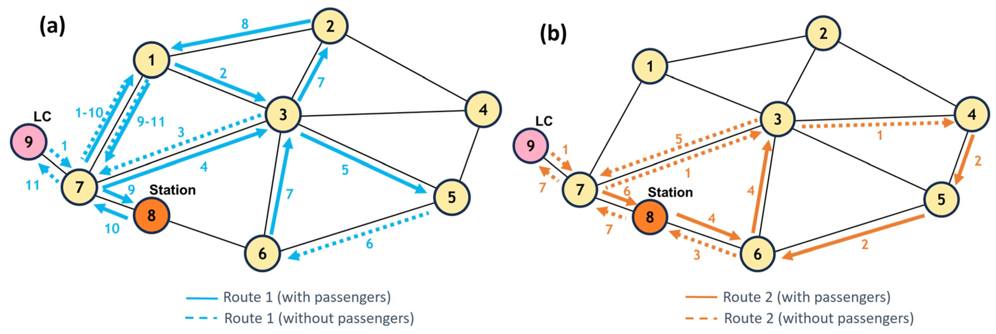
3.1. Definition of the Routes of the DRT System

In this section, the routes of the DRT system are obtained for each scenario, indicating the demand satisfied and not satisfied. An example is shown in Figure 4 with the routes’ solution for the DRT system in a specific scenario E_02_2C4. Scenario E_02_2C4 has two vehicles of four seats each; the O-D matrix considered is of 12 trips with 31 passengers, and the maximum waiting time (t_m) is 30 min (see O-D matrix in Table 2).

Figure 4 shows the routes followed by the two available vehicles in the scenario, beginning and finishing their trips in the logistics centre (LC). Route 1 (Figure 4a) performs a DRT service comprising seven trip requests (POP 1 to POP 3, POP 7 to POP 3, POP 3 to POP 5, POP 6 to POP 2, POP 2 to Station, POP 1 to Station and Station to POP 1), and Route 2 (Figure 4b) performs a DRT service comprising three trip requests (POP 4 to POP 6, Station to POP 3 and POP 7 to Station). The numbers in Figure 4 and Figure 5 represent each movement of the vehicle in each route. In addition, there are two travel demands of scenario E_02_2C that have not been satisfied by the DRT system (see more details in Figure 5).

Figure 5a shows the same routes (Routes 1 and 2) in scenario E_02_2C4, with more details about the schedules. In this scenario, we need to highlight that the travel demand is the highest mainly between 9:00 and 15:30 in the O-D matrix. The demand schedules should be studied to be able to adjust the DRT service schedules and set the margin for this service throughout the day. In this graph, the parallelograms represent the time windows of each trip request when users are willing to make the trip. Similarly to in Figure 4, the continuous lines represent the movement of a route with passengers onboard, while the discontinuous lines represent route movements without passengers onboard. Then, the numbers in the links indicate the step of the total movements made in each route. The stops in each route are represented by blue and white circles, respectively. In Figure 5a, there are two circles in each stop, showing that the arrival and departure are delayed by 5 min, the time established as a service time for passengers getting on and off the vehicle.

Focusing on each particular trip and analysing the demand schedules and real schedules, Figure 5b shows a demand trip that has a pick-up time window between 9:18 and 9:48 at POP 1, and an arrival-time window between 9.30 and 10.00 at POP 3. Under these conditions, the DRT system can satisfy this demand. However, there are two travel requests in this scenario that are not satisfied (POP 5 to Station and Station to POP 4 in Figure 5c). This lack of service is because some conditions cannot be fulfilled; in particular, the service within the time windows and the number of vehicles/capacities (number of seats). Finally, although most of the satisfied trips do not share the vehicle during their journey, there are two cases, trips 5 and 6, shown in Figure 5d. The DRT system picks up passengers from trip 5 in POP 2 at 13.19, and then drives to POP 1 to pick up passengers from trip 6 at 12.49. Finally, they go together to the station, which is the destination of both trips.

3.2. Evaluation of Different Scenarios

In the next section, we perform a sensitivity analysis, but first let us evaluate the performance of the system in the different scenarios using the weight factors shown in

Table 8. Values of the weight of evaluation.

Values of Weight
α1	α2	α3	β	γ
0.50	0.10	0.05	0.20	0.15

, meaning that, for a particular case, the social factor has a greater weight than the economic and environmental ones in the decision-making process.

The scores of all the scenarios have been represented in the following figures for the three assumed levels of demand, i.e., matrix of 12, 25 and 50 trips (Figure 6, Figure 7 and Figure 8, respectively). These graphs represent the scenarios by the mean of the sum of capacities of the assumed vehicles on the x-axis, and the score P from 0 to 10 on the y-axis. The analysis of these three figures is performed jointly, presenting a comparative assessment of the results shown for the three levels of demand:

• The number of trips demanded directly influences the total score obtained. A comparison of the three graphs shows how for the demands of the 12 trips (Figure 6), the average score is higher than in the case of the higher demand of the 25 trips (Figure 7), and this is higher than in case of the 50 trips (Figure 8), regardless of the capacity offered. DRT systems work without limitations for lower demand, giving service to all the travel requests in most cases, as a taxi service; while for higher requests, the system starts to decrease in efficiency.
• The number of vehicles increases the score values up to a certain limit, which depends on the number of trips demanded. In general, the increase in the vehicles’ fleet converges at a certain score, which means increasing the number of vehicles does not provide better service to users, and the system would be oversupplied. For example, Figure 6 shows that having more than three vehicles does not increase the final score, similarly to in Figure 7 (O-D matrix of 25 trips), where that limit is achieved for five vehicles.
• Regarding the sum of the capacities (seats offered), the graphs show that increasing the sum of the capacities (y-axis in the graphs) of the DRT system is only interesting if it is associated with the number of vehicles. For example, Figure 6 shows that the case of a maximum waiting time (t_m) of 20 min and with a sum of capacity of 9 seats (one vehicle) has a lower score than the case with two vehicles of 4 seats (sum of the capacity of 8 seats). A similar case could be found if we compare the cases of two vehicles of 22 seats (sum of capacity of 44 seats) with a sum of the capacity of 22 seats (three vehicles in total). The latter presents better performance. In summary, in rural areas where the travel demand is reduced, vehicles with many seats available only increase costs and have no influence on the quality of the service, decreasing the final scores.
• The parameter of the maximum waiting time (t_m) has a significant influence on the DRT scores. If t_m increases, there is generally an increase in the score. For example, in Figure 6, the red lines (t_m 20 min) have lower scores than the green lines (t_m 30 min), and these have lower scores than the blue lines (t_m 40 min). This parameter could be as efficient as the number of vehicles, producing in some cases a higher increase in the DRT scores. For instance, some scenarios in Figure 8 with t_m of 20 min with four vehicles have lower scores than other scenarios with t_m of 30 or 40 min with three vehicles. This means the DRT services could arrive in a wider time window, servicing more requests. However, an increasing t_m is also related to a longer waiting time assumed by potential users and, therefore, DRT systems need to find a proper balance between efficiency (final scores) and the quality offered.

3.3. Sensitivity Analysis of Weight Factors

After evaluating the different scenarios, we performed a sensitivity analysis to identify how the weighting factors adopted for each indicator could influence the P score of the DRT systems. This sensitivity analysis evaluates ten cases with different weighting factors (

Table 9. Values of the weight in the sensitivity analysis.

Cases of Sensibility Analysis
CASE 1	CASE 2	CASE 3	CASE 4	CASE 5
α1 = 0.50	α1 = 0.50	α1 = 0.50	α1 = 0.35	α1 = 0.35
α2 = 0.10	α2 = 0.10	α2 = 0.10	α2 = 0.10	α2 = 0.10
α3 = 0.05	α3 = 0.05	α3 = 0.05	α3 = 0.05	α3 = 0.05
β = 0.20	β = 0	β =0.35	β = 0.5	β = 0
γ = 0.15	γ = 0.35	γ = 0	γ = 0	γ = 0.50
CASE 6	CASE 7	CASE 8	CASE 9	CASE 10
α1 = 0.35	α1 = 0.65	α1 = 0.65	α1 = 0.65	α1 = 0.85
α2 = 0.1	α2 = 0.10	α2 = 0.10	α2 = 0.10	α2 = 0.10
α3 = 0.05	α3 = 0.05	α3 = 0.05	α3 = 0.05	α3 = 0.05
β = 0.25	β = 0	β = 0.2	β = 0.1	β = 0
γ = 0.25	γ = 0.20	γ = 0	γ = 0.1	γ = 0

). The values of these parameters have been chosen so the social aspect (α₁ + α₂ + α₃) could range between 0.5 and 1.0, while both the economic and environmental dimensions (β and γ) have weights between 0 and 0.5, forcing α₁ + α₂ + α₃ + β + γ = 1. These values have been adapted to ensure that the social aspect, related to providing service to users, acquires a minimum of 0.5, guaranteeing that the quality of the service reaches a minimum to improve the quality of public transport services in rural areas where there are no other alternatives in many cases.

The method for comparing the results in this sensitivity analysis uses statistical deciles. This means 10 percent of the scenarios with the highest P-score in each of the 10 proposed cases were selected (18 out of 174 scenarios for each O-D matrix).

Table 10. Top 3 scenarios with the highest scores in the sensitivity analysis.

Matrix	Top 1		Top 2		Top 3
12 trips	E_03_3C4 E_04_4C4	9/10	E_05_5C4	7/10	E_20_1C4_2C9 E_29_2C4_1C9 E_33_2C4_1C22	6/10
25 trips	E_05_5C4	8/10	E_06_6C4 E_58_4C4_1C9_1C22	7/10	E_04_4C4 E_37_3C4_3C9	6/10
50 trips	E_06_6C4 E_37_3C4_3C9	9/10	E_05_5C4 E_57_3C4_2C9_1C22 E_58_4C4_1C9_1C22	7/10	E_23_1C4_5C9 E_32_2C4_4C9	6/10
Total	E_04_4C4	10/10	E_03_3C4 E_05_5C4 E_06_6C4 E_37_3C4_3C9 E_48_3C4_1C9_1C22	9/10	E_58_4C4_1C9_1C22	8/10

shows the scenarios that are included more times in the first decile for each combination of weighting factors, showing the three options with the highest ratios (Top 1, 2 and 3). In the case that several scenarios have the same percentage, all of them are shown. For example, in a particular case for an O-D matrix of 12 trips, the scenarios that appear most times (9 out of 10 total cases) in the first decile of the DRT system’s best scores are scenarios E_03_3C4 (three vehicles with a capacity of four seats) and E_04_4C4 (four vehicles with a capacity of four seats).

From this sensitivity analysis, we obtained the following key insights:

• For all the proposed cases with different weight factors, scenarios with lower and medium capacities (four and nine seats) achieve better P-score values for different levels of demand and in total. There is no case in the Top 1 where a vehicle with a capacity of 22 seats appears. For this reason, in rural areas, where the demand and population density are low and dispersed, vehicles with small or medium capacity would have a better performance.
• The analysis of the Top 1 of the three matrices shows an increase in the number of vehicles servicing higher demands but maintaining their capacity in most cases. This means the parameter of the number of vehicles is much more influential than their capacity in these rural environments.
• Focusing on the total results in Table 10 (without differencing among the matrices of demand), we observe that scenario E_04_4C4 is always included as an efficient solution (10 out of 10), thus becoming a potential candidate for a DRT system to be implemented in the proposed theoretical network.
• For these kinds of services, the social dimension must have higher relevance to ensure a certain level of service, prioritising options in which the number of passengers served is as high as possible, while the economic and environmental aspects are kept as low as possible. Therefore, despite the changes in the weight factors, the scenarios are usually repeated in most of the cases analysed.

The proposed four-step method, combined with the sensibility analysis, would allow us to define DRT systems for inter-urban mobility in rural areas, identify the factors influencing the final performance of potential solutions, and subsequently vary the criteria according to the operator and management of the transport system in each context.

4. Discussion and Conclusions

This paper provides a systematic method to guide the implementation of demand-responsive transport (DRT) systems for inter-urban long-distance mobility in rural areas and identifies the influence of different factors on the final performance of the service. The research examines different solutions for implementing DRT services, considering a set of simulated scenarios in which different factors, such as the number of vehicles, fleet capacity, and maximum waiting times assumed by users are evaluated.

In general, this paper provides some important insights. First, in rural areas where the travel demand is lower than in urban areas, low- and medium-capacity vehicles perform better, cost less and provide the same quality of service. Second, the allocation of time windows in the travel demand should incorporate the option of setting the pick-up time at the point of origin or the arrival time at the destination. Third, the flexibility of users’ requirements in terms of the maximum time they are assumed to wait (t_m) notably influences the number of travel demands the DRT system can satisfy. This parameter must be evaluated jointly with the design of the fleet because both influence the quality of service. These results are in coherence with the existing literature on the topic, which states that DRT systems could be considered an interesting alternative to traditional public transport systems based on fixed lines and services [4,12,14,17]. In addition, the analysed factors of the number of vehicles and their capacity are usually considered in the route optimisation methods proposed by other authors [26], particularly in rural areas with low population density and long distances between them. Finally, in this research, the importance of waiting times is highlighted (as also evidenced by other authors [24,32]), including an analysis of the real waiting times and those willing to wait through the parameter of maximum waiting time (t_m). Although other studies support some of the insights in this paper, most of them are oriented towards optimisation and lack a broad, critical assessment of the influence of different factors on the final performance of DRTs in rural areas.

In summary, this research offers a useful method for transport planners and regional authorities to implement DRT services adapted to inter-urban mobility in rural areas and the particularities of these geographies. Accordingly, our study fills a gap in the literature, which neglects to analyse the factors influencing the efficiency of this transport alternative in these areas. The proposed GIS-based method presents a systematic evaluation and analysis of the factors that influence the DRT service. It needs to be adapted to each specific context regarding the network configurations, but the procedure for selecting and evaluating the most adequate DRT solution for each case study provides a useful tool, allowing for the adaptation of the weighting factors depending on the administration and planners’ interests. This could have relevant policy implications for the design and evaluation of DRT systems implemented in rural areas. A key aspect that future research could address would be to validate the findings by comparing them with empirical data from real DRT implementations. Nowadays, the data available from open sources about pilot cases of DRT implementation in rural areas are very limited (or even inexistent), which makes a direct comparison very difficult. Further exploration, and contacts and agreements with administrations, will help in accessing this valuable information. In addition, the application of the method proposed to real case studies will be studied, considering the existing demand and a real background.

References

1. Martínez Sánchez-Mateos, H.S.M.; Ruiz Pulpón, A.R. Closeness is Not Accessibility: Isolation and Depopulated Rural Areas in the Proximity of Metropolitan Urban Areas, A Case-Study in Inland Spain. Eur. Countrys. 2021, 13, 410–435. [Google Scholar] [CrossRef]
2. Pinilla, V.; Ayuda, M.I.; Sáez, L.A. Rural Depopulation and the Migration Turnaround In Mediterranean Western Europe: A Case Study of Aragon. J. Rural. Community Dev. 2008, 3, 1–22. [Google Scholar]
3. Viñas, C.D. Depopulation processes in European Rural Areas: A case study of Cantabria (Spain). Eur. Countrys. 2019, 11, 341–369. [Google Scholar] [CrossRef]
4. Vitale Brovarone, E.; Cotella, G. Improving rural accessibility: A multilayer approach. Sustainability 2020, 12, 2876. [Google Scholar] [CrossRef]
5. Burkhardt, J.E.; Hamby, B.; McGavock, A.T.; United States Federal Transit Administration; Transit Cooperative Research Program; Transit Development Corporation. Users’ Manual for Assessing Service-Delivery Systems for Rural Passenger Transportation; National Academy Press: Washington, DC, USA, 1995.
6. Mulley, C.; Daniels, R. Quantifying the role of a flexible transport service in reducing the accessibility gap in low density areas: A case-study in north-west Sydney. Res. Transp. Bus. Manag. 2012, 3, 12–23. [Google Scholar] [CrossRef]
7. Mageean, J.; Nelson, J.D. The evaluation of demand responsive transport services in Europe. J. Transp. Geogr. 2003, 11, 255–270. [Google Scholar] [CrossRef]
8. Park, S.; Xu, Y.; Jiang, L.; Chen, Z.; Huang, S. Spatial structures of tourism destinations: A trajectory data mining approach leveraging mobile big data. Ann. Tour. Res. 2020, 84, 102973. [Google Scholar] [CrossRef]
9. Türk, U.; Östh, J.; Kourtit, K.; Nijkamp, P. The path of least resistance explaining tourist mobility patterns in destination areas using Airbnb data. J. Transp. Geogr. 2021, 94, 103130. [Google Scholar] [CrossRef]
10. Li, X.; Quadrifoglio, L. Feeder transit services: Choosing between fixed and demand responsive policy. Transp. Res. Part C Emerg. Technol. 2010, 18, 770–780. [Google Scholar] [CrossRef]
11. Moyano, A.; Tejero-Beteta, C.; Sánchez-Cambronero, S. Mobility-as-a-Service (MaaS) and High-Speed Rail Operators: Do Not Let the Train Pass! Sustainability 2023, 15, 8474. [Google Scholar] [CrossRef]
12. Coutinho, F.M.; van Oort, N.; Christoforou, Z.; Alonso-González, M.J.; Cats, O.; Hoogendoorn, S. Impacts of replacing a fixed public transport line by a demand responsive transport system: Case study of a rural area in Amsterdam. Res. Transp. Econ. 2020, 83, 100910. [Google Scholar] [CrossRef]
13. Campisi, T.; Cocuzza, E.; Ignaccolo, M.; Inturri, G.; Tesoriere, G.; Canale, A. Detailing DRT users in Europe over the last twenty years: A literature overview. Transp. Res. Procedia 2023, 69, 727–734. [Google Scholar] [CrossRef]
14. ESPON Programme. Urban-Rural Connectivity in Non-Metropolitan Regions (URRUC) Synthesis Report [Internet]. 2019. Available online: www.espon.eu (accessed on 1 April 2024).
15. Navidi, Z.; Ronald, N.; Winter, S. Comparison between ad-hoc demand responsive and conventional transit: A simulation study. Public Transp. 2018, 10, 147–167. [Google Scholar] [CrossRef]
16. Sörensen, L.; Bossert, A.; Jokinen, J.P.; Schlüter, J. How much flexibility does rural public transport need?—Implications from a fully flexible DRT system. Transp. Policy 2021, 100, 5–20. [Google Scholar] [CrossRef]
17. König, A.; Grippenkoven, J. The actual demand behind demand-responsive transport: Assessing behavioral intention to use DRT systems in two rural areas in Germany. Case Stud. Transp. Policy 2020, 8, 954–962. [Google Scholar] [CrossRef]
18. Giuffrida, N.; Le Pira, M.; Inturri, G.; Ignaccolo, M. Addressing the public transport ridership/coverage dilemma in small cities: A spatial approach. Case Stud. Transp. Policy 2021, 9, 12–21. [Google Scholar] [CrossRef]
19. Dytckov, S.; Persson, J.A.; Lorig, F.; Davidsson, P. Potential Benefits of Demand Responsive Transport in Rural Areas: A Simulation Study in Lolland, Denmark. Sustainability 2022, 14, 3252. [Google Scholar] [CrossRef]
20. Yen, B.T.H.; Mulley, C.; Yeh, C.J. Performance evaluation for demand responsive transport services: A two-stage bootstrap-DEA and ordinary least square approach. Res. Transp. Bus. Manag. 2023, 46, 100869. [Google Scholar] [CrossRef]
21. Wang, C.; Quddus, M.; Enoch, M.; Ryley, T.; Davison, L. Exploring the propensity to travel by demand responsive transport in the rural area of Lincolnshire in England. Case Stud. Transp. Policy 2015, 3, 129–136. [Google Scholar] [CrossRef]
22. Laporte, G. The Vehicle Routing Problem: An overview of exact and approximate algorithms. Eur. J. Oper. Res. 1992, 59, 345–358. [Google Scholar] [CrossRef]
23. Fisher, M.L. Optimal Solution of Vehicle Routing Problems Using Minimum K-Trees. Oper. Res. 1993, 42, 626–642. [Google Scholar] [CrossRef]
24. Mahmoudi, M.; Zhou, X. Finding optimal solutions for vehicle routing problem with pickup and delivery services with time windows: A dynamic programming approach based on state-space-time network representations. Transp. Res. Part B Methodol. 2016, 89, 19–42. [Google Scholar] [CrossRef]
25. Zhou, X.; Tong, L.; Mahmoudi, M.; Zhuge, L.; Yao, Y.; Zhang, Y.; Shang, P.; Liu, J.; Shi, T. Open-source VRPLite Package for Vehicle Routing with Pickup and Delivery: A Path Finding Engine for Scheduled Transportation Systems. Urban Rail Transit 2018, 4, 68–85. [Google Scholar] [CrossRef]
26. Guo, R.; Guan, W.; Zhang, W.; Meng, F.; Zhang, Z. Customized bus routing problem with time window restrictions: Model and case study. Transp. A Transp. Sci. 2019, 15, 1804–1824. [Google Scholar] [CrossRef]
27. Enrique Fernández, L.J.; de Cea Ch, J.; Malbran, R.H. Demand responsive urban public transport system design: Methodology and application. Transp. Res. Part A Policy Pract. 2008, 42, 951–972. [Google Scholar] [CrossRef]
28. Shen, S.; Ouyang, Y.; Ren, S.; Chen, M.; Zhao, L. Design and implementation of zone-to-zone demand responsive transportation systems. Transp. Res. Rec. 2021, 2675, 275–287. [Google Scholar] [CrossRef]
29. Van Oort, N.; Van Der Bijl, R.; Verhoof, F.; Coffeng, G. The wider benefits of high quality public transport for cities. In Proceedings of the European Transport Conference, Barcelona, Spain, 4–6 October 2017. [Google Scholar]
30. Grunicke, C.; Schlüter, J.; Jokinen, J.P. Evaluation methods and governance practices of new flexible passenger transport projects. Res. Transp. Bus. Manag. 2021, 38, 100575. [Google Scholar] [CrossRef]
31. Ma, W.; Zeng, L.; An, K. Dynamic vehicle routing problem for flexible buses considering stochastic requests. Transp. Res. Part C Emerg. Technol. 2023, 148, 104030. [Google Scholar] [CrossRef]
32. Avermann, N.; Schlüter, J. Determinants of customer satisfaction with a true door-to-door DRT service in rural Germany. Res. Transp. Bus. Manag. 2019, 32, 100420. [Google Scholar] [CrossRef]
Figure 1. Steps of the method proposed.
Ijgi 13 00275 g001
Figure 2. Toy network.
Ijgi 13 00275 g002
Figure 3. Description of the steps of the proposed method.
Ijgi 13 00275 g003
Figure 4. Routes’ optimal solution for scenario E_02_2C4. (a) Route 1. (b) Route 2.
Ijgi 13 00275 g004
Figure 5. (a) Routes’ optimal solution for scenario E_02_2C4. (b) Satisfied demand trip directly. (c) Non-satisfied demand trip. (d) Satisfied demand trips, travelling together with other demand trip.
Ijgi 13 00275 g005
Figure 6. P score for scenarios of 12-trip matrices.
Ijgi 13 00275 g006
Figure 7. P score for scenarios of 25-trip matrices.
Ijgi 13 00275 g007
Figure 8. P score for scenarios of 50-trip matrices.
Ijgi 13 00275 g008